Long-Term Spatial Load Forecasting Using Human-Machine Co-construct Intelligence Framework

(1)

ABSTRACT

HONG, TAO. Long-Term Spatial Load Forecasting Using Human-Machine Co-construct Intelligence Framework. (Under the direction of Dr. Simon Hsiang).

This thesis presents a formal study of the long-term spatial load forecasting problem: given small area based electric load history of the service territory, current and future land use information, return forecast load of the next 20 years. A hierarchical S-curve trending method is developed to conduct the basic forecast. Due to uncertainties of the electric load data, the results from the computerized program may conflict with the nature of the load growth. Sometimes, the computerized program is not aware of the local development because the land use data lacks such information. A human-machine co-construct intelligence

framework is proposed to improve the robustness and reasonability of the purely

(2)

Long-Term Spatial Load Forecasting

Using Human-Machine Co-construct Intelligence Framework

by Tao Hong

A thesis submitted to the Graduate Faculty of North Carolina State University

In partial fulfillment of the Requirements for the degree of

Master of Science

Operations Research and

Industrial & System Engineering

Raleigh, North Carolina Oct. 2008

APPROVED BY:

_______________________________ ______________________________

Simon Hsiang Shu-Cherng Fang

Committee Chair

(3)

ii

DEDICATION

(4)

iii

BIOGRAPHY

(5)

iv

ACKNOWLEDGEMENTS

I would like to thank my mother, Ms. Baohui Yin, and father, Mr. Jinmin Hong, for their continuous support, mentally and financially, for my studies abroad. I would like to thank my fiancée, Ms. Pu Wang, for her love, encouragement and tolerance.

I would like to thank my advisor Dr. Simon Hsiang, for his precious time and valuable advice during the past two years. Dr. Hsiang’s enthusiasm for research and diligent working attitude has been a great example to me. I would like to thank Dr. Yahya Fathi, for accepting my application to the Operations Research program, for helping me with the tedious paper work required for my enrollment, and for serving on my committee. I would like to thank Dr. Shu-Cherng Fang for serving on my committee and for offering me a cubical in his group so that I didn’t feel lonely or desperate while I’m working on my thesis. I would like to thank my former advisor, Dr. Mo-Yuen Chow for helping me to develop the ability of independent thinking.

I would like to thank my former roommate, former lab-mate, and present officemate, Dr. Le Xu, for picking me up from RDU airport when I first came to Raleigh, helping me settle down during the first year at NC State, for sharing with me his insights on research, and for guiding me to complete my first spatial load forecasting project, which had lead to this thesis.

(6)

v James Burke, for advising me on the principles of being an engineer, for teaching me the fundamentals of power distribution systems, and for helping build my expertise in this field. I would like to thank my colleagues, Mr. Lee Willis, Mr. Philips Edmunds, and Ms. Jia Wang, from Quanta Technology for the support and suggestions they gave during the load forecasting projects.

(7)

vi

LIST OF TABLES

(10)

ix

LIST OF FIGURES

Figure 1.1 Map of Madison, WI ... 2

Figure 1.2 Electric load distribution of Madison, WI ... 3

Figure 1.3 Load growth distribution of Madison, WI... 3

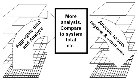
Figure 1.4 Bottom-up aggregation & top-down allocation... 11

Figure 2.1 An automated computer program structure of hierarchical trending method ... 13

Figure 2.2 Typical data format of transformer based historical load... 17

Figure 2.3 Typical data format for weather normalization ... 18

Figure 2.4 Land use code ... 19

Figure 2.5 Current land use data ... 20

Figure 2.6 Future land use data... 20

Figure 2.7 Small area based historical load data... 21

Figure 2.8 Service territory map ... 22

Figure 2.9 Weather normalized load vs. actual load... 23

Figure 2.10 Effect of HYL on the overall forecast (1) ... 26

Figure 2.11 Effect of HYL on the overall forecast (2) ... 26

Figure 2.12 Neighborhood table ... 29

Figure 2.13 Potential amount of sub-regions in each level... 31

Figure 2.14 Bottom-up aggregation... 33

Figure 2.15 S-curve shapes affected by HYL parameter ... 34

(11)

x

Figure 2.17 S-curve shapes affected by ramp up time parameter... 35

Figure 2.18 Top-down allocation... 37

Figure 3.1 A semi-automated hierarchical trending method with HMCCI framework... 41

Figure 4.1 “Initialization” worksheet... 52

Figure 4.2 “Weather Normalization” worksheet ... 54

Figure 4.3 “All Data” worksheet – weather normalized historical load ... 55

Figure 4.4 “HYL Solver” worksheet ... 56

Figure 4.5 “Service Territory” worksheet... 58

Figure 4.6 “Service Territory” worksheet – information board... 58

Figure 4.7 Temporary results of bottom-up aggregation ... 61

Figure 4.8 “Bottom-Up Solver” worksheet ... 62

Figure 4.9 “Top-Down Solver” worksheet ... 62

Figure 4.10 “Result Display Setup” worksheet ... 63

Figure 4.11 “Forecast Incremental Load” worksheet ... 64

Figure 4.12 “Forecast Actual Load” worksheet... 64

Figure 4.13 “Forecast Map” worksheet ... 65

Figure 4.14 Forecast map selection ... 66

Figure 4.15 Forecast incremental load map (2010) ... 66

(12)

1

1 Introduction

1.1 Overview of Spatial Load Forecasting

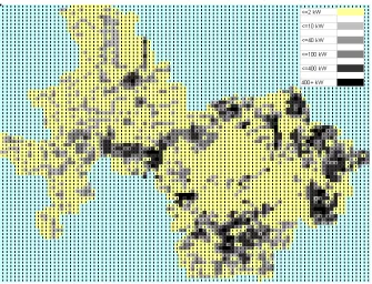
If quality is defined by what the customers want, one way to measure the success of an electric power distribution system is to deliver reliable electric power to customers spread throughout utility’s service territory. Figure 1.1 shows a Google map of Madison in Wisconsin, and Figure 1.2 shows its electric load distribution, which contains a pattern that is typical of a medium-sized city in the United States.

1) There is high load density in and around the central business district (downtown) area, while a lower density in the outlying suburban areas.

2) Even in the suburbs, the load density along the major industrial areas can be higher than that of the downtown areas which are filled with residential customers and office parks.

3) In rural areas, load density is very low because homes, commercial areas, and industrial areas are spread far apart.

4) Due to the use of irrigation pumps and oil pumps in petroleum fields, the load density can be surprisingly high in comparison with other rural areas.

(13)

2 sufficient accuracy to allow for quality planning of electric power transmission and distribution facilities. Assessing the impacts of alternatives for conjunctive areas also requires attention to processes the possibilities that take place on different spatial and temporal scales. Information scale is the spatial and temporal scale of the information required. Generally, a strategic resources manager (for example the local, regional or national government) needs information on a scale relative to their responsibilities and authorities. This level of information is likely to differ from the level desired by operational managers dealing with day-to-day issues. Information at scales smaller than what is needed is seen as being ‘noisy’. Information at scales larger than what is needed is not relevant or helpful. Specifically, in load forecasting, the scale, or resolution, of the map is also depends on the computing capability to generate historical load data.

Dow

ntow

n

(14)

3

Figure 1.2 Electric load distribution of Madison, WI

(15)

4 The spatial information is addressed by using the small area forecast method: the utility service territory is divided into many, perhaps thousands of small areas, and a forecast is done for each.

(16)

5

1.2 Decision Making Process

Based on his/her domain knowledge (e.g., social, economic, or political background), one planner is usually assigned to a certain region in service territory. In every planning period, this planner submits an expansion plan that includes what equipment to maintain, purchase, and install based on his/her experience, e.g., what development activities he/she has seen and heard of in the past, the historical load data and outages that have occured in this region, the construction-limit land information, etc. After all the planners submit their proposals, the director or higher level managers in charge of planning will make the final decision considering the trade off between benefit and cost, and then allocate a budget to each region accordingly. A comprehensive planning process can be found in Chapter 26 of [23].

(17)

6 A rather simple technique that can reach absurd conclusions if incorrectly applied is to equate the benefits of a service to the cost of supplying the service by the least expensive alternative method. Thus the benefits from hydroelectricity generation could be estimated as the cost of generating that electricity by the least cost alternative method using solar, wind, geothermal, coal-fired, natural gas or nuclear energy sources. Clearly, this approach to benefit estimation is only valid if, were the project not adopted, the service in question would in fact be demanded at, and supplied by, the least-cost alternative method. The pitfalls associated with this method of benefit and cost estimation can be avoided if one clearly identifies reasonable with and without project scenarios.

(18)

7

1.3 Literature Review

As load forecasting is highly related to the quality of system planning, attention has been paid to the impact of load forecasting on system design [24] and economics [20]. A system wide two-stage distribution planning algorithm is reported in [19]. Optimization software [4] and techniques [10] are applied to load forecasting as well as planning. Load forecasting is usually tied to reliability analysis [3, 35, 36] and distribution transformer load management (TLM) [5].

There are dozens of different distribution load forecasting methods that have been used and documented during the last 50 years. Some of them fall into the category of short-term forecasting [12, 16], which is beyond the scope of this thesis. Some of them are long-term forecasting methods, the majority of which are spatial load forecasting methods [25, 26]. In [29], the authors summarized and compared 14 different distribution forecasting methods which appeared during the 1960s to early 1980s. Some spatial load forecasting methods can be used for transmission planning as well [11, 34]. As the development of computer technologies and applications ramped up in the 1980s, many computer based load forecasting methods were being developed [17, 21, 33]. Data issues and database development were paid attention to during the same period [22], followed by the discussion of information integration issues in distribution planning [37].

(19)

re-8 development [7, 8, 9]; a knowledge-based expert system has been designed for fast developing utility’s long-term load forecasting [15]; an extended logistic model was used for high growth load forecasting as well [1]; a method to take care of rural area load forecast was reported in [27]; the load transfer issue has been investigated in [32]; forecasting under uncertainties has been discussed in [31]; neural networks have been applied to forecasting wind speed for long-term load forecasting [2]; the data mining approach has been used for spatial modeling [14]; a load survey system was used to determine customer load characteristics [6]; some fast algorithms have been developed to reduce computer running time [28, 30].

Despite various methods, algorithms, computer codes/programs in use, all fall into three basic types of methods: trending [28], simulation [18] and the hybrid method:

1) Trending methods look for some function to fit the past load growth patterns and estimate the future load based on the function. The most common trending method is to use multivariate regression to fit a polynomial function to load history data. This approach has a number of failings when applied to spatial load forecasting, while dozens of improved methods have been reported for load forecasting. The advantages of the trending method include ease of use, simplicity, and a short-range response to recent trends of load growth patterns. However, it often fails to have a useful estimate of the long-range load.

(20)

9 future load growth. Simulation methods usually simulate an urban development process based on land-use change information from government, customer rate class from utilities, and load curve model of consumption patterns. Depending on the quality of data, this approach has a fair to very good short-range accuracy. Depending on the specific algorithm, this approach has a good to excellent long-range usefulness for planning. The drawback of the simulation method is the expensive development and training cost.

3) Hybrid trending-simulation methods combine features of trending and simulation. An ideal hybrid method should well respond well to recent trends of load history in the short-range, and keep the long-range accuracy as simulation methods have. Meanwhile, the ideal hybrid method should be easy to use, and not require much interaction and skills from the user. That ideal may be unattainable, but it is certainly worth pursuing.

(21)

10 Quantitative models can help inform interested stakeholders and those individuals or agencies responsible for recommending or making decisions or policy. The merit and advantages, as well as the limitations, of various quantitative methods for analysing various planning or management issues are generally recognized throughout the community. The assumptions and uncertainties associated with any model-generated impact predictions should be understood and considered by those using these model predictions.

(22)

11

Figure 1.4 Bottom-up aggregation & top-down allocation

(23)

12

1.4 Organization of the Thesis

(24)

13

2 Hierarchical Trending Method

2.1 Overall Program Structure

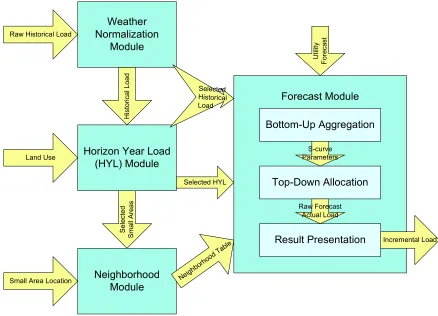
In this chapter, a hierarchical trending method using S-curve has been investigated and developed. Figure 2.1 shows an automated computer program structure.

Raw Historical Load

Land Use

Small Area Location

Weather Normalization

Module

Horizon Year Load (HYL) Module Neighborhood Module H ist o ri ca l L o a d Selected HYL Neigh borh ood Table Forecast Module Bottom-Up Aggregation Top-Down Allocation Result Presentation S-curve Parameters Raw Forecast Actual Load Incremental Load S e le ct e d S m a ll A re a s Selected Historical Load U ti lit y F o re ca st

(25)

14 As shown in Figure 2.1, the arrows represent data flow, while the rectangular blocks represent functional modules:

1) Weather normalization module: this module applies a utility’s weather normalization method to the raw historical load data to generate the adjusted historical load. Different utility companies may have different weather normalization methods, which mainly fall into various regressions.

2) Horizon year load (HYL) module: this module takes land use data and adjusted historical load data to generate load densities for each land use type as well as the HYL for each small area. It then selects the small areas with higher HYL than the current load as the areas of interest to forecast the load growth on.

3) Neighborhood module: this module builds the neighborhood table according to the total number and the location, sometimes together with load information as well, of the selected areas of interest.

(26)

(27)

16

2.2 Data Outlook

Compared with simulation data, real-world data provided by utilities has a lot more uncertainties, noise and errors, which create difficulties for the forecasting. Before starting the forecast algorithm development, several typical data sets obtainable from utilities are introduced in this section.

2.2.1 Historical Load

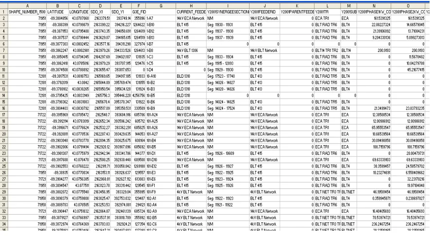
Figure 2.2 shows the data format of transformer based historical load information that most utilities can provide, which contains the following two sets:

1) Geographical information: In the geographical information system (GIS), the surface of the earth has been cut into many small areas according to a certain scheme (e.g., 1500ft by 1500ft). Each small area has a unique shape number, which is shown in column A of Figure 2.2. The location of a transformer in the small area can be represented by latitude and longitude, or another coordination scheme specified by a particular GIS. As shown in Figure 2.2, Columns B and C represent the longitude and latitude of the corresponding transformer, while Columns D and E represent its coordinate in feet.

2) Load history: Load history information and details of the transformer (e.g., feeder number, voltage level, etc.) are listed after geographical information, from which the load history on a small area basis will be extracted.

(28)

17

Figure 2.2 Typical data format of transformer based historical load

2.2.2 Weather Normalization

(29)

18 1) Maximum temperature records the highest temperature that appeared during the year

of interest.

2) Cooling Degree Days (CDD) describes how much a period’s weather should result in a building’s cooling requirements. The hotter the day is, the more the CDD is. If the amount of CDD is double, then this should result in roughly double the cooling requirements for a building. CDD is calculated individually for each day. CDD over a month or billing cycle are merely a summation of CDD of the individual days.

3) Employment shows the number of employees or job positions in the service territory. Sometimes it can be replaced by number of customers if the utility company has customer count data in the service territory.

(30)

19 2.2.3 Horizon Year Load

A land used based approach to calculate horizon year load (HYL) will be proposed in section 2.4. This approach requires a land use code and current and future land use information:

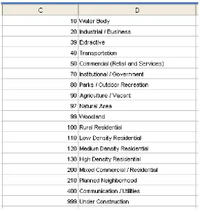
A land use code describes the purpose of land use or customer types within the small area, e.g., commercial, industrial, low-density residential, high-density residential, water body, etc. All types are coded using numbers as shown in Figure 2.4.

Figure 2.4 Land use code

(31)

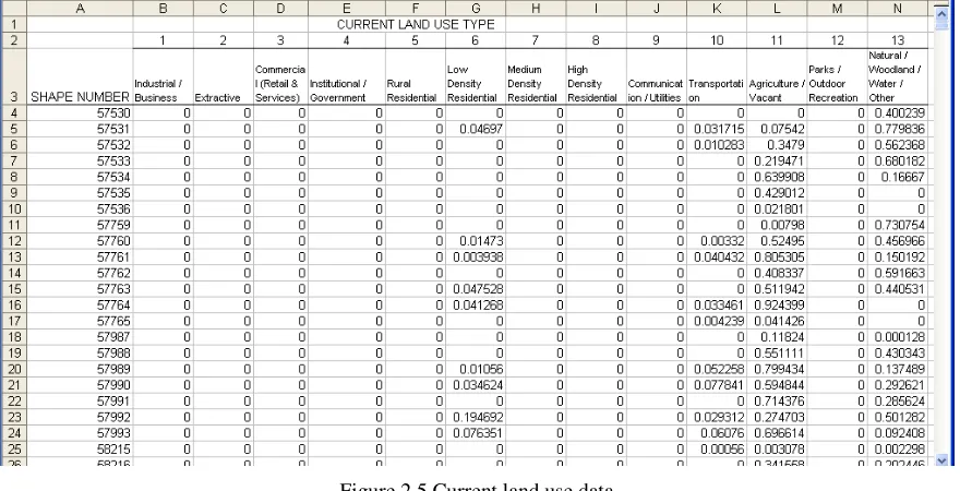
20 and future land use information are required to calculate HYL. The data format of current land use is shown in Figure 2.5, while future land use has exactly the same format as shown in Figure 2.6.

Figure 2.5 Current land use data

(32)

21

2.3 Data Preprocessing

2.3.1 Small Area Based Historical Load

The first step of data preprocessing is to convert transformer based load data to small area based load data and assign coordinates to each small area. The extraction procedure is the following:

1) Rank the shape numbers of all the small areas from low to high;

2) Define the reference point for each small area, e.g., the upper-left corner;

3) Add the load of transformers with the same shape number together, the result of which is the historical load for this small area.

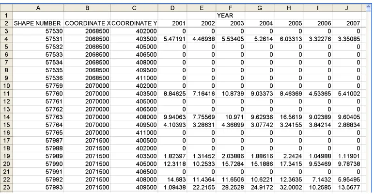
As shown in Figure 2.7, column B and C show the coordinates of the reference point in a small area, while columns D to J are small area based annual peak load data from 2001 to 2007, the unit of which is kW.

(33)

22 2.3.2 Service Territory Map

According to the coordinates of small areas, a service territory map can be drawn as the light yellow area in Figure 2.8. In the beginning stage, the service territory map can be used to verify the data quality. Sometimes due to errors from a data source, some regions may not appear in the map correctly. By comparing the generated map with the real map, one can tell approximately whether the service territory has been correctly represented.

Figure 2.8 Service territory map

2.3.3 Weather Normalization

(34)

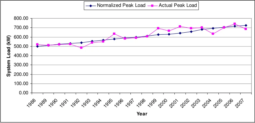
23 and employment (x₃), the natural log of which are denoted as y, x₁, x₂, and x₃ respectively. The least square method is used to calculate the coefficient (k₁, k₂, and k₃) of a line to best fit the given data, the formula of which is

y=k₁x₁+k₂x₂ +k₃x₃ (2.1) The weather normalized system load ( 'y ) is shown as the blue curve in Figure 2.9, while the purple curve represents the actual load.

0.00 100.00 200.00 300.00 400.00 500.00 600.00 700.00 800.00 19 88 19 89 19 90 19 91 19 92 19 93 19 94 19 95 19 96 19 97 19 98 19 99 20 00 20 01 20 02 20 03 20 04 20 05 20 06 20 07 Year S y s te m L o a d ( k W )

Normalized Peak Load Actual Peak Load

Figure 2.9 Weather normalized load vs. actual load

The coefficient ci is used to normalize small area load of a particular year i, and can be calculated by: i i i y y c '

= , (2.2)

where y_i is the actual system load of year i, and '

i

(35)

24 And the normalized load is equal to the actual historical load data multiplied by the coefficient c_i:

ij i ij cL

L' = , (2.3)

where Lij is the actual historical load of a small area j in year i, and

'

ij

(36)

25

2.4 Determining Horizon Year Load Using Land Use Information

Horizon year load (HYL) describes the load of a fully saturated small area. In long-range spatial load forecast, an estimate of the farthest forecast year load can be considered as HYL, although the land may be further developed or redeveloped after the forecast range. It is crucial to get a quality HYL for a useful forecast. Figure 2.10 and Figure 2.11 show how different HYLs affect the forecast given the same historical data.

(37)

26

Effect of HYL (1)

0 10 20 30 40 50 60 70 80 20 01 20 02 20 03 20 04 20 05 20 06 20 07 20 08 20 09 20 10 20 11 20 12 20 13 20 14 20 15 20 16 20 17 20 18 20 19 20 20 Year # L o a d ( k W

) Historical Data

HYL = 10 kW

HYL = 20 kW

HYL = 50 kW

HYL = 80 kW

Figure 2.10 Effect of HYL on the overall forecast (1)

Effect of HYL (2)

0 2 4 6 8 10 12 14 16 18

200 1

200 2

200 3

200 4

200 5

200 6

200 7

200 8

200 9

201 0

201 1

201 2

201 3

201 4

201 5

201 6

201 7

201 8

201 9

202 0 Year # L o a d ( k W

) Historical Data

HYL = 10 kW

HYL = 12 kW HYL = 14 kW

HYL = 16 kW

Figure 2.11 Effect of HYL on the overall forecast (2)

(38)

27 method to determine HYL is introduced. An implementation in MS Excel is described as follows:

The land use types are divided into 10 to 15 categories based on physical meaning of data (e.g., group different factories as industrial land use). Original land use data from a given county may includes 20 or even more types, which is inefficient for calculation, while 10 to 15 categories are fewer and more practical considering both the computational complexity and the quality of the results.

The load density variables (d_k, k = 1, 2, 3…) are set for each category, and are used to calculate the load of the most recent historical year (known as base year b) for each small area by multiplying load density with current land use:

∑

⋅

=

k

kj k

bj d CLU

Lˆ' ( ), (2.4)

where Lˆ'_bj is the calculated base year load of small area j, d_k is the load density of category k, and CLU_kj is the acreage of current land use category k in small area j.

To solve the optimization formulation using Excel add-in Solver, tune the load density variables to minimize the sum of square errors between the calculated base year load and the weather normalized base year load with the constraint of non-negative load density:

Min:

∑

−

j

bj bj L

Lˆ' ' )2

(39)

28 s.t. d_k ≥0, k = 1, 2, 3, … (2.5)

Calculate the mismatch Ej between the calculated and weather normalized base year load:

' '

ˆ bj bj j L L

E = − , (2.6)

Multiply the calculated load density with future land use, and then add the mismatch calculated from step 4 to the result from step 5 to get the adjusted load of horizon year, which is HYL.

j k

kj k

j d FLU E

HYL =

∑

( ⋅ )+ , (2.7)

where FLUkj is the acreage of future land use category k in small area j.

(40)

29

2.5 Neighborhood Module

In the hierarchical trending method, small areas are aggregated from bottom to top and the system-wide load is distributed from top to bottom. During this process, small areas within the same neighborhood are aggregated, and the load of the upper level region will be allocated to the small areas within the same neighborhood as well. Neighbor here may not be geographically adjacent, but a scheme exists to group the small areas or sub regions in each level. The neighborhood table (Figure 2.12) is the link of this iterative method. This section introduces a simple but robust approach to build a neighborhood table.

(41)

30 The neighborhood table is a table of indices of sub-regions. As shown in Figure 2.12, the columns represent the levels from bottom to top, and each entry represents the sub-region index in the corresponding level. For example, column B represents the 2nd level bottom-up, and cell B7 represents the 2nd region in level #2. In this neighborhood table, small areas #1 through #5 in level #1 form sub-region #1 in level #2, sub-regions #1 through #4 in level #2 form sub-region #1 in level #3, and so forth. In each level, every sub-region should include the same amount (4 or 5) of sub-regions in the lower level, though this is not a hard requirement.

With the above considerations, the procedure of building a neighborhood table is described as follows:

1) Determine a load growth threshold as the just noticeable difference for load forecasting. In other words, if the horizon year load is no more than the sum of this threshold and the base year load, planners can consider that there is no growth in this small area through the forecast range.

(42)

31 3) Determine the number of small areas that will be considered for forecast. This number is the smallest potential sub-region number that includes all small areas whose mismatches are above the threshold.

4) Assign indices to the selected small areas. In the binary tree, trace from level #1 to the root to build the neighborhood table using the multiplier (4 or 5).

5 25 100 125 500 625 400 3125 2500 2000 1600 20 80 320 1280 4 16 64 256 1024 1 Level #1 Level #2 Level #3 Level #4 Level #5 Level #6

(43)

32

2.6 Bottom-Up Aggregation: S-curve Parameter Tuning

Historical load and horizon year load of the small areas within each neighborhood are aggregated from the bottom level to the top level as shown in Figure 2.14. In each level, S-curve is used to fit the corresponding data from each small area (bottom level) or sub-region (second level or higher). During this bottom-up aggregation, the S-curve fitting is a crucial segment, the results of which will be the starting point for each small area or sub-region of top-down allocation. Parameter tuning of S-curve will be discussed in the following sections.

2.6.1 Format of S-curve

The typical format of S-curve (Gompertz function) can be written as:

ct

be

ae t

y( )= , (2.8)

where a is the upper asymptote, c is the growth rate, and b and c are negative numbers. This typical format can be adopted as:

ec(t b c)

ae t

y( )= − +ln(−)/ . (2.9)

Let

) ln( 1

b c t=− −

(44)

33

Figure 2.14 Bottom-up aggregation

Formula (2.9) is equivalent to:

) (

)

(t ae ect t

y = − −∆ , (2.11)

where a is the HYL of a small area, c is the load growth rate, and ∆t is the ramp up time.

(45)

34 important to the users (planners) because the parameter tuning process can be easily visualized. Therefore, formula (2.11) has been used to represent S-curve in this thesis. For example, the ramp up time depends upon both b and c in (2.8), while in (2.11) it is determined by _∆t only.

Figure 2.15 shows how the shape of S-curve is affected by tuning HYL parameter a: the S-curve is stretched vertically as the HYL parameter is increasing. Figure 2.16 shows how the shape of S-curve is affected by slope parameter c: the S-curve is stretched horizontally as the absolute value of c is decreasing. As the slope is approaching zero, the S-curve tends to become a straight line. Figure 2.17 shows how the shape of S-curve is affected by ramp up time parameter ∆t: the S-curve moving from the left to the right as ∆t is increasing.

c = -0.3, delta t = 0

-20 0 20 40 60 80 100 120

-15 -5 5 15 25 35

Time

L

o

a

d

a = 100 a = 90 a = 80 a = 70 a = 60

(46)

35

a = 100, delta t = 0

-20 0 20 40 60 80 100 120

-15 -5 5 15 25 35

Time

L

o

a

d

c = -0.5 c = -0.4 c = -0.3 c = -0.2 c = -0.1

Figure 2.16 S-curve shapes affected by slope parameter

a = 100, c = -0.3

-20 0 20 40 60 80 100 120

-15 -5 5 15 25 35

Time

L

o

a

d

delta t = -5 delta t = 0 delta t = 5 delta t = 10 delta t = 15

(47)

36 2.6.2 Problem formulation

Bottom-up aggregation involves two elements:

1) Aggregate the historical load and HYL of the neighborhood small areas or sub-regions to obtain the historical load and HYL of the sub-region in the upper level. 2) Fit the historical load data of a small area or sub-region given the HYL using S-curve,

which can be modeled as an optimization problem:

Min:

∑

(

)

= − − ∆ − H t e t h ae H t t c 1 2 ) (

1 ( )

s.t. c≤_0, _(2.12)

where H is the length of historical load, and h(t) is the historical load of the tth year. This step is to tune the slope and shift the curve horizontally to find the best match with the historical load.

2.7 Top-Down Allocation: Multi-objective Optimization

Compared with the decision making process introduced in section 1.2, bottom-up aggregation simulates regional planners’ forecasting process, while top-down allocation is like distributing the corporation forecast load growth to sub-regions in lower levels, and even down to the small areas in the bottom level (Figure 2.18). There are several goals during this process:

1) Generated S-curves should match the correspondent historical load.

(48)

37 3) Since the development period of regions with the same size is similar, the slope of

small areas of sub-regions in the same level should be close. 4) The load in the farthest forecast year should be close to HYL.

Figure 2.18 Top-down allocation

The corporation forecast load of the future years will be used in the top level to drive top-down allocation. To achieve the above goals, a multi-objective optimization approach is applied, where the first two are put into objectives, and the latter two are put into constraints:

1) Minimize historical load mismatch Fi:

(

)

∑

= − − = −∆ H t i e i

i ae h t

H

F cit ti

1

2

) (

1 ( )

, i = 1, 2, …, K (2.13)

where K is the number of neighbors in one neighborhood in a given level. 2) Minimize future load mismatch G:

∑ ∑

+ = = − _      − − = −∆ N H t K i e

ie f t

a H

N

G ci t ti

1 2 1 ) ( ) (

1 ( )

(49)

38 where N is the total number of years including the historical years, and f(t) is the forecasted load of correspondent sub-region in the upper level.

3) Slope boundary: Cmin ≤ci ≤Cmax , where Cmaxand Cmin represent the upper bound

and lower bound of the slope.

4) Ramp up time boundary: ∆t_min ≤∆t_i ≤∆t_max.

To sum up, each allocation unit can be formulated as:

Min: M F M G

K

i

i 2 1

1

∑

+

=

s.t. C_min ≤ci ≤C_max,

∆tmin ≤∆ti≤∆tmax,

where M1 and M2 are the penalty factors for historical load mismatch and upper level future

forecasted load mismatch respectively. In practice, M1 is set to be much larger than M2 to

(50)

39

3 Human-Machine Co-construct Intelligence

3.1 Motivation

Although the automated computer program is convenient for users, the results lack common judgment. For instance, it may produce a higher load density of residential customers than industrial customers, which is intuitively incorrect to a distribution planner. Since there are many such rules based on planners’ experience, it’s neither efficient nor feasible to input all of them as constraints into the program. As an enhancement, a human expert is integrated into the problem solving loop to provide heuristics and insights to correct or confirm the results from the computer. The iterative calibration process, in which human and machine work together and negotiate with each other to come up with a solution, is named as human machine co-construct intelligence (HMCCI). Figure 3.1 shows a semi-automated program structure with the HMCCI framework implemented in the HYL module and the overall procedure illustrated.

(51)

40 the particular approach to objective identification and quantification and to plan selection that is most appropriate.

The method deemed most appropriate for a particular situation will depend not only on the physical scale of the situation itself but also on the decision-makers, the decision-making process, and the responsibilities accepted by the analysts, the participants and the decision-makers.

Finally, because that the decisions being made at the current time are only part of a sequence of decisions that will be made on into the future. No one can predict with certainty what future generations will consider as being important or what they will want to do, but spending some time trying to guess is not an idle exercise. It pays to plan ahead, as best one can, and ask ourselves if the decisions being considered today will be those we think our descendants would have wanted us to make. This kind of thinking gets us into issues of adaptive management and sustainability

(52)

41 H ist o ri ca l L o a d Neigh borh ood Table S e le ct e d S m a ll A re a s U ti lit y F o re ca st

(53)

42

3.2 Determining Load Densities Using Greedy HMCCI

3.2.1 Greedy Selection Procedure

As discussed in Section 2.4, load densities are calculated as intermediate results using current land use information and base year load, and HYL can be determined based on these load densities and future land use information. An optimization problem is formulated to calculate the load densities. Table 3.1 shows the resulting load densities when different amounts (from 100% to 99.0%) of the small areas are taken into consideration. Notice that all of these densities are equally reasonable to a computer running the optimization problem formulated in Section 2.4. However, an experienced distribution planner can understand the extensive physical meanings about these numbers and help the computer to select a more suitable set of load densities, or critique the current solutions to pursue better ones.

Table 3.1 Load densities for selection procedure

Land Use Information Load Density (kW/acre)

Index Land Use Type

Current Acreage

Future

Acreage 100.0% 99.8% 99.5% 99.0%

1 Industrial / Business 2490 4820 45.57 37.26 31.24 28.55

2 Extractive 1060 394 0.00 0.00 0.00 0.00

3 Commercial (Retail & Services) 4025 6204 34.30 39.29 37.60 40.41

4 Institutional / Government 2791 2733 45.89 26.71 24.04 22.25

5 Rural Residential 358 5553 31.54 4.55 9.92 11.74

6 Low Density Residential 16696 17446 2.64 4.81 6.26 6.58

7 Medium Density Residential 894 1607 36.62 35.49 31.21 32.84

8 High Density Residential 2525 3137 30.78 26.93 25.86 25.77

9 Communication / Utilities 695 673 13.53 15.68 15.89 4.83

10 Transportation 15372 16174 10.45 8.80 6.08 4.56

11 Agriculture / Vacant 66699 47679 0.00 0.00 0.00 0.00

12 Parks / Outdoor Recreation 5697 6802 0.00 0.27 0.65 0.96

(54)

43 A greedy algorithm tries to find a local minimum at each stage of the problem with the hope of reaching a global optimum at the end. Although most of the time greedy algorithms fail to find the global optimum, they often produce a reasonably good approximation of the global optimum within a short time. Various greedy algorithms have been developed to solve NP-complete problems. However, due to the partial information utilized in each stage, computerized greedy algorithms may even reach the worst solution sometimes. This is definitely undesirable to some critical applications including load forecasting, because a bad forecast may lead to a disaster in a city and create much damage to the society. In this section, a human expert is put into the loop of the greedy strategy to have an overall control of the results in order to avoid worst case scenarios, or to even improve the results from the purely computerized program.

A greedy selection procedure can be described as following:

1) Find out the agreed upon observations among all the candidate solution sets. Highlight the observations using the color green, and exclude them from the future decision making.

2) Rank the significance of the remaining observations from more significant to less significant. If all of the remaining observations are similarly significant, just place them in any sequence.

(55)

44 move to the next one, until all the observations have been checked or there is only one solution set with no red mark. The remaining one or more solution sets without red mark will be the preferred choices.

The key argument here is that the good enough subset and the selected subset. Informally, a good enough subset is a subset of the search space in which the members satisfy some planning criteria set forth by the decision maker. Oftentimes, a good enough subset is easy to specify but difficult to obtain by the machine intelligence. In contrast, the selected subset is a subset in which the members are picked out by the human intelligence using certain evaluation analogies or metaphors as the outcome for the planning process. Every optimization problem can, in principle, be conceived as the goal of matching a selected subset with the good enough subset. Take Table 3.1 as an example:

1) All the solution sets agree that land use types #1, #11, and #13 have zero load densities, which are highlighted in green.

2) Suppose the remaining land use types are equally significant, so they are placed as they are numbered.

3) The load density of land use type #4 calculated by 100% small areas is marked as red, because it is significantly higher than the others.

4) The load density of land use type #5 calculated by 100% small areas is marked as red, because it is significantly higher than the others.

(56)

45 6) The load density of land use type #9 calculated by 99% small areas is marked as red,

because it is significantly lower than the others.

7) Therefore, load densities calculated by 99.5% small areas are selected as a reasonable solution set for further calculation of HYL.

3.2.2 Greedy Critique Procedure

Although the selection procedure allows a planner to select the best solution set in his/her mind among all the solution sets provided by the computer, it may still fail when none of the computer-provided solution sets are reasonable or when part of the solution sets have considerable drawbacks. A critique procedure can overcome such a failed scenario:

1) Starting with a solution set, find out the agreement between the planner and the computer. Mark the corresponding variables using the color green, make them as constants, and exclude them from the optimizations.

2) Among the remaining variables, find the most disagreed on variable, change its value, mark it as yellow, make is as a constant, and exclude it from the optimizations.

3) Tune the remaining variables to minimize the mismatches. If the all of the resulting densities are colored by green or yellow, use them to compute HYL. Otherwise, go back to step (1).

(57)

46 Table 3.2 shows a mock critique process starting with the calculation of 99.5% small areas, where the agreed upon values are highlighted in green and the manually modified values are highlighted in yellow:

1) The planner agrees with the load densities of land use type #2, #11, #12, and #13. 2) The planner changes the load density of transportation from 6.08kW/acre to

2.00kW/acre.

3) Among the resulting load densities, the planner agrees on land use type #1, #7, #8, and #9.

4) The planner changes the load density of the rural residential customers from 11.56kW/acre to 7.64kW/acre.

5) The planner agrees with none of the remaining resulting load densities.

6) The planner changes the load density of the commercial customers from 46kW/acre to 38kW/acre.

7) The planner is satisfied with all of the load densities. The load density results can be used in the HYL calculation.

(58)

47

Table 3.2 Using critique procedure to calculate load densities

Index Land Use Type

Step 1

Step 2

Step 3

Step 4

Step 5

Step 6

Step 7

1 Industrial / Business 31.24 31.24 29.59 29.59 29.59 29.59 29.59

2 Extractive 0.00 0.00 0.00 0.00 0.00 0.00 0.00

3 Commercial (Retail & Services) 37.60 37.60 44.79 44.79 46.00 38.00 38.00

4 Institutional / Government 24.04 24.04 19.97 19.97 18.02 18.02 19.20

5 Rural Residential 9.92 9.92 11.56 7.64 7.64 7.64 7.64

6 Low Density Residential 6.26 6.26 7.64 7.64 7.73 7.73 7.73

7 Medium Density Residential 31.21 31.21 34.88 34.88 34.88 34.88 34.88

8 High Density Residential 25.86 25.86 27.85 27.85 27.85 27.85 27.85

9 Communication / Utilities 15.89 15.89 17.05 17.05 17.05 17.05 17.05

10 Transportation 6.08 2.00 2.00 2.00 2.00 2.00 2.00

11 Agriculture / Vacant 0.00 0.00 0.00 0.00 0.00 0.00 0.00

12 Parks / Outdoor Recreation 0.65 0.65 0.65 0.65 0.65 0.65 0.65

(59)

48

3.3 Customized Scenarios

Although well-tuned load densities can provide overall matching with the current load of most of the small areas, in a few small areas, which are treated as outliers, there may be some local rules that differ a lot from the calculated load densities. Even among the small areas used in the optimization problem, the variance of mismatches is still very large due to the local information that a computer program doesn’t have. Therefore, such information has to come from the local planners.

Furthermore, because of the multitude of factors that determine demand, perfect forecasting of economic development and resulting demands is a utopian dream. Future demands are often dependent on future scenarios. An electric load demand scenario is a logical combination of basic parameters of the economy. An understanding of the functioning of the socio-economic system, based on the human expert knowledge developed through the assessment of past and present trends should be used to formulate a limited number of consistent scenarios. Therefore, integration of planners’ local knowledge is essential for a useful forecast.

3.3.1 Revising Horizon Year Load

(60)

49 reflected by land use information, because land use is the same as before. Therefore, the computer program is not able to indentify such growth. In this case, the planner can simply increase the HYL to include the load growth introduced by an increased number of computers.

Since HYL is calculated through land use data and base year load, land use data can affect the HYL as well. It is possible that errors exist in the land use data, which will lead to a wrong forecast if the error is significant. By looking at the forecast maps, a planner can tell by intuition whether the forecast is reasonable or not. For example, the forecast map may show that there is some load growth on a lake, which is a water body that has a zero load density. When checking the future land use data, the planner finds that some residential land use is misplaced on the lake. In this case, the planner can correct the land use data by erasing the residential land on the map.

3.3.2 Adding New Business Information

(61)

(62)

51

4 Implementation and Results

The whole algorithm has been implemented in Microsoft Office Excel 2003 Visual Basic for Applications with Solver add-in. This chapter is devoted to introducing the implementation, Graphical User Interface (GUI), and related results.

4.1 Initialization

Some basic information is necessary to initialize the tool, which is put into the “Initialization” worksheet as shown in Figure 4.1.

In this worksheet, a planner needs to input the following information:

1) Names of the utility company and the planner. These two names will not be used in the program, but are for documentation purpose.

2) Temporal information that includes the base year, length of historical data, and forecast range. The first two will be used to generate the header of “Load History” worksheet (Figure 2.7).

(63)

52 4) Corporation forecast. The planner can use a common percentage as the approximate

corporation forecast, or specify the load growth of each year.

Figure 4.1 “Initialization” worksheet

(64)

(65)

54

4.2 Weather Normalization

Weather normalization is conducted after inputting the historical load, and current and future land use information. “Weather Normalization” is a stand-alone worksheet as shown in Figure 4.2. The data for calculation has been entered and hidden to the user.

Figure 4.2 “Weather Normalization” worksheet

As introduced in Section 2.2.2, weather normalization applies a multivariate regression approach to calculate the coefficient for each historical year. There are four functional buttons in the “Weather Normalization” worksheet:

1) Clear Form: Delete all the data in this table.

2) Reset Form: Copy the pre-entered hidden data to the table.

(66)

55 4) Apply Weather Normalization Parameters: Multiply the raw historical load from the “Load History” worksheet by the corresponding coefficient and output the weather normalized load to the “All Data” worksheet as shown in Figure 4.3.

(67)

56

4.3 Horizon Year Load Solver

The HYL of each small area is calculated in the “HYL Solver” worksheet as shown in Figure 4.4. There are four functional buttons:

1) Initialize HYL Solver: Copy necessary data, such as the base year load, and the current and future land use data to the present worksheet. Then calculate a statistical summary (e.g., current and future acreage of each land use type) and set up formulas to prepare for Solver’s optimization. Finally copy current and future land use data to the “All Data” worksheet.

2) Calculate HYL: Run Solver twice to get the load densities as well as the HYL. All small areas are used for optimization the first time, and a user-determined percentage of small areas is used at the second time.

3) Apply HYL: Copy calculated HYL to the “All Data” worksheet.

4) Reset Form: Delete all the data and reset the form back to its original status.

(68)

57

4.4 Service Territory Map

The “Service Territory” worksheet (Figure 4.5) has the following four functions:

1) Show service territory map and detailed small area information, such as historical load, HYL, and current and future land use.

2) Allow user to edit future land use and HYL. 3) Allow user to add new business or development.

4) Allow user to select different accurate level to run engine.

The territory should often coincide with an administrative unit (region, district, county etc.), because the administrative system usually requires an analysis of the functioning of the resources within its administrative boundaries. The system boundaries however, depend on its physical characteristics. They include the administrative area, but may extend over a larger area, depending upon the physical boundaries.

(69)

58

Figure 4.5 “Service Territory” worksheet

Figure 4.6 “Service Territory” worksheet – information board

There are five buttons on the information board:

1) Generate Map: Draw service territory map based on small area coordinates in “All Data” worksheet.

(70)

59 3) Change HYL: A planner can change future land use data and HYL which are the cells filled with the color white. The modified HYL will be copied to the “All Data” worksheet to update the old one.

4) Add New Business: This row contains cells for new business land use, start year, and end year that are shown as white cells on the board. A planner can fill in the blanks with the corresponding new business information.

5) Calculate NB load: A new business load will be fit into an S-curve based on the planner’s input, and then put into the “New Business Load” worksheet.

Other than the five buttons, there are three check boxes on the information board as well. These boxes are used to select a forecast threshold, which is used to determine whether a small area’s load is considered as growth. If the mismatch between the HYL and the base year load is above the threshold, then the small area’s load can be considered as growth, and vice versa. Table 4.1 shows the approximate time under different forecast speed settings when the program is running on a computer with Intel Core 2 Duo 2.2GHz CPU and 2G RAM.

Table 4.1 Computer run time under different forecast speed settings

Check Box Threshold (kW) Amount of small areas Time (min)

Fast Forecast 10 1024 50

Medium Forecast 5 1280 60

Slow Forecast 0 3460 110

(71)

60 reduce the resolution of small areas, e.g., from 51.66 acres to 206.64 acres. Both of them will sacrifice the accuracy of the forecast.

(72)

61

4.5 Engine

4.5.1 Bottom-Up Aggregation

The small areas’ historical load and the HYL are aggregated from bottom level to top level, and the data of each level are stored in a different workbook called “Level id” (“id” is replaced by the level index) as shown in Figure 4.7, where the first column is the index of the small area, the last column is HYL, and the middle columns are the load of historical years.

Figure 4.7 Temporary results of bottom-up aggregation

(73)

62

Figure 4.8 “Bottom-Up Solver” worksheet

4.5.2 Top-Down Allocation

The top-down allocation is also implemented in a single worksheet named “Top-Down Solver” as shown in Figure 4.9. The upper level forecast data is copied from the corresponding “Level id” worksheet, and the initial value of the S-curves parameters are copied from the “Curve id” worksheet. After the Solver finishes the calculation for each sub-region’s load allocation, the forecast results will be copied to the corresponding “Level id” worksheet. All the worksheets generated by the engine, including the “Bottom-Up Solver” worksheet, “Top-Down Solver” worksheet, “Level id” worksheets, and “Curve id” worksheets (other than “level1” worksheet), will be deleted after the top-down allocation is finished.

(74)

63

4.6 Forecast Results

4.6.1 Result Display Setup

A planner can select some particular years or all years within the forecast range to display forecast results in the “Result Display Setup” worksheet (Figure 4.10) by selecting one of the two check boxes.

(75)

64 4.6.2 Final Forecast Results

Final forecast results are presented in both data format and map format. Data format includes the incremental load (Figure 4.11) and the actual load (Figure 4.12). The incremental load is the load growth compared with the base year. If the growth is less than the threshold pre-determined in the “Service Territory” worksheet, it is treated as equal to the threshold. The actual load is the sum of the incremental load and the base year load.

Figure 4.11 “Forecast Incremental Load” worksheet

(76)

65 The “Forecast Map” worksheet is shown in Figure 4.13. In the upper-left corner, which is shown in larger detail Figure 4.14, the planner can select which year to look at and whether to view the incremental or actual load map. For instance, Figure 4.15 and Figure 4.16 show the incremental load map and the actual load map of 2009’s forecast results respectively. In both maps, the darker the color code is, the more load or load growth the small area has.

(77)

66

Figure 4.14 Forecast map selection

(78)

67

(79)

68

5 Conclusion and Future Work

5.1 Conclusion

This thesis presents a tool for long-range spatial load forecasting. A hierarchical trending method has been investigated and implemented. An advanced feature, HMCCI, has been proposed to integrate human planners into the decision making process. The proposed method has been applied to several utilities and has received satisfactory results. Compared with most existing methods and tools in the literature and industry, the tool presented has the following advantages:

1) Easy to set up. The required user inputs can be extracted easily from most utilities’ databases.

2) Short run time. It takes less than two hours to get the results for a service territory with 3400 small areas. Moreover, the run time can be further reduced by selecting a higher load growth threshold.

3) Short training period. It takes one business day to train the planners to understand the basic forecast concept, master the tool and produce forecast results.

(80)

(81)

70

5.2 Future Work

Although the proposed tool has provided useful results for some utilities with limited budgets and resources for load forecasting, there are still several research topics that need to be further investigated in order to perfect the tool.

The current neighborhood table is built based on total number of small areas without the consideration of geographical information. The grouping of the nearest small areas or the small areas with similar land use types might be helpful to the forecast. The investigation of different grouping methods is expected to be one way to improve the current work.

(82)

71

References

1 Barakat, E.E.; Al-Rashed, S.A., "Long range peak demand forecasting under conditions of high growth," IEEE Transactions on Power Systems, vol.7, no.4, pp.1483-1486, Nov 1992

2 Barbounis, T.G.; Theocharis, J.B.; Alexiadis, M.C.; Dokopoulos, P.S., "Long-term wind speed and power forecasting using local recurrent neural network models,"

IEEE Transaction on Energy Conversion, vol.21, no.1, pp. 273-284, March 2006 3 Billinton, R.; Dange Huang, "Effects of Load Forecast Uncertainty on Bulk Electric

System Reliability Evaluation," IEEE Transactions on Power Systems, vol.23, no.2, pp.418-425, May 2008

4 Blanchard, M.; Delorme, L.; Simard, C.; Nadeau, Y., "Experience with optimization software for distribution system planning," IEEE Transactions on Power Systems, vol.11, no.4, pp.1891-1898, Nov 1996

5 Yen-Ting Chao; Sheng-Ta Lee; Hong-Chan Chang; Tsai-Hsiang Chen, "An

improvement project for distribution transformer load management in Taiwan," IEEE Transactions on Power Systems, vol.18, no.2, pp. 875-881, May 2003

6 Chen, C.S.; Hwang, J.C.; Tzeng, Y.M.; Huang, C.W.; Cho, M.Y., "Determination of customer load characteristics by load survey system at Taipower," IEEE Transactions on Power Delivery, vol.11, no.3, pp.1430-1436, Jul 1996

7 Chow, M.-Y.; Tram, H., "Methodology of urban re-development considerations in spatial load forecasting," IEEE Transactions on Power Systems, vol.12, no.2, pp.996-1001, May 1997

8 Chow, M.-Y.; Tram, H., "Application of fuzzy logic technology for spatial load forecasting," IEEE Transactions on Power Systems, vol.12, no.3, pp.1360-1366, Aug 1997

9 Mo-Yuen Chow; Jinxiang Zhu; Tram, H., "Application of fuzzy multi-objective decision making in spatial load forecasting," IEEE Transactions on Power Systems, vol.13, no.3, pp.1185-1190, Aug 1998

(83)

72 11 de la Torre, S.; Conejo, A.J.; Contreras, J., "Transmission Expansion Planning in

Electricity Markets," IEEE Transactions on Power Systems, vol.23, no.1, pp.238-248, Feb. 2008

12 Gross, G.; Galiana, F.D., "Short-term load forecasting," Proceedings of the IEEE, vol.75, no.12, pp. 1558-1573, Dec. 1987

13 Hill, D.C.; Infield, D.G., "Modelled operation of the Shetland Islands power system comparing computational and human operators' load forecasts," IEE Proceedings-Generation, Transmission and Distribution, vol.142, no.6, pp.555-559, Nov 1995 14 Hung-Chih Wu; Chan-Nan Lu, "A data mining approach for spatial modeling in small

area load forecast," IEEE Transactions on Power Systems, vol.17, no.2, pp.516-521, May 2002

15 Kandil, M.S.; El-Debeiky, S.M.; Hasanien, N.E., "Long-term load forecasting for fast developing utility using a knowledge-based expert system," IEEE Transactions on Power Systems, vol.17, no.2, pp.491-496, May 2002

16 Moghram, I.; Rahman, S., "Analysis and evaluation of five short-term load

forecasting techniques," IEEE Transactions on Power Systems, vol.4, no.4, pp.1484-1491, Nov 1989

17 Palayanon, Visnu; Sinsawad, Arthorn; Juramongkorn, Borvorn; Willis, H. L.; Powell, R. W.; Tram, H. N., "Computerized Distribution Load Forecast for the City of

Bangkok," IEEE Transactions on Power Systems, vol.2, no.1, pp.218-225, Feb. 1987 18 Powers, M.W., "The analytical Monte Carlo method for approximating the

distribution of a plant's electrical generation," IEEE Transaction on Energy Conversion, vol.3, no.3, pp.433-439, Sep 1988

19 Quintana, V.H.; Temraz, H.K.; Hipel, K.W., "Two-stage power-system-distribution-planning algorithm," IEE Proceedings-Generation, Transmission and Distribution, vol.140, no.1, pp.17-29, Jan 1993

20 Ranaweera, D.K.; Karady, G.G.; Farmer, R.G., "Economic impact analysis of load forecasting," IEEE Transactions on Power Systems, vol.12, no.3, pp.1388-1392, Aug 1997

Long-Term Spatial Load Forecasting Using Human-Machine Co-construct Intelligence Framework

DEDICATION

BIOGRAPHY

ACKNOWLEDGEMENTS

TABLE OF CONTENTS

LIST OF TABLES

LIST OF FIGURES

1

Introduction

1.1

Overview of Spatial Load Forecasting

1.2

Decision Making Process

1.3

Literature Review

1.4

Organization of the Thesis

2

Hierarchical Trending Method

2.1

Overall Program Structure

2.2

Data Outlook

2.3

Data Preprocessing

2.4

Determining Horizon Year Load Using Land Use Information

∑

∑

∑

2.5

Neighborhood Module

2.6

Bottom-Up Aggregation: S-curve Parameter Tuning

∑

(

)

2.7

Top-Down Allocation: Multi-objective Optimization

(

)

∑

∑ ∑

∑

3

Human-Machine Co-construct Intelligence

3.1

Motivation

3.2

Determining Load Densities Using Greedy HMCCI

3.3

Customized Scenarios

4

Implementation and Results

4.1

Initialization

4.2

Weather Normalization

4.3

Horizon Year Load Solver

4.4

Service Territory Map

4.5

Engine

4.6

Forecast Results

5

Conclusion and Future Work

5.1

Conclusion

5.2

Future Work

References