Hard x ray observations of the extragalactic sky: the High Energy Focusing Telescope and the Serendipitous Extragalactic X ray Source Identification survey

Energy Focusing Telescope and the Serendipitous

Extragalactic X-ray Source Identification survey

Thesis by Peter Hsih-Jen Mao

In Partial Fulfillment of the Requirements for the Degree of

Doctor of Philosophy

California Institute of Technology Pasadena, California

2002

c

Acknowledgments

You learn what you don’t know you are learning.

—Gian-Carlo Rota

Luck comes to the well prepared.

—Steven Frautschi

As an undergraduate, I was told that one’s graduate school experience is far more dependent on the advisor than the school itself. Indeed, I have had a wonderful time here, and I attribute much of it to my advisor, Fiona Harrison. In my first few weeks at Caltech, I took David Hogg’s advice to talk to many different professors before picking a research group. Tom Prince told me about a project to design high energy x-ray mirrors that Fiona, who was in Australia flying a balloon, would be taking the lead on. The project sounded interesting to me, but, having never met her, I had no idea how Fiona would be as an advisor and she had no idea how I would be as a student. Tom relayed my interest in the project to her, she agreed to take me as a student, and things have worked out pretty well. Fiona has given me opportunities to meet and work with many talented, interesting and fun scientists all over the world. She has given me the leeway to develop my own style of doing science, while at the same time making sure that my graduate education has been well rounded. I have copious tales of her generosity, but they would only serve to embarrass her.

My first trip with Fiona was to the Motor City, to begin multilayer fabrication tests with Osmic, Inc. There, I worked with Yuriy Platonov, Luis Gomez, David Broadway, and Brian DeGroot (who left Osmic to take over his family’s pig farm in Canada). All of the mirror fabrication that I directly had a hand in happened at Osmic with Yuriy, Luis, David, and Brian, and I thank them for their patience, hospitality, and generosity in sharing their knowledge and experience. I remember remarking to Fiona on that first trip that I thought Detroit would be an interesting place to live. She didn’t agree.

stolen from a Boca Raton airport later that year.

The Danish Space Research Institute is part of the HEFT collaboration, responsible for the coating of the flight optics. Our cohorts in Denmark include Finn Christensen, the Danish cowboy, Ahsen Hussain, his incorruptible graduate student, and Carsten Jensen, his very corruptible post-doc. A few weeks after Deirdre and I got married, Fiona sent me off to Denmark to characterize some mirrors that we had coated at Osmic. Finn thought this was a bad idea, since the last time a collaborator had come to Copenhagen, the collaborator broke off his engagement. Deirdre and I are still married. On that trip, I worked with Ahsen, Karsten Joensen, Finn’s former student on whose work mine builds, and the Italians Carlo Pelliciari and Giovanni Pareschi. Giovanni has a great story about an encounter he had with a stranger in Lyon, France.

Copenhagen is the home of Hans Christian Andersen and one of its landmarks is the statue of the Little Mermaid. I visited the site of the statue on Thanksgiving. After I returned to the States, I heard that some vandals had cut her head off.

At the 1998 Physics of X-ray Multilayer Structures conference in Breckenridge, CO, I first met David Windt, at the time a researcher at Bell Laboratories. David invited me to work with him for a few weeks at Bell Labs. This was a key event in my graduate career. Following discussions with David, I reorganized my approach to multilayer design and this eventually led to the figure of merit and optimization methods described in this thesis. David has since left Bell Labs to join the HEFT collaboration at Columbia University.

The multilayer optimization software also owes its existence to Tom Prince, Stuart Andersen, and Leon Bellan. Tom helped me get access to the Caltech Advanced Computing Resource’s massively parallel supercomputers and Stuart showed me the ins and outs of parallel computing. In the summer of 1999, I was lucky to procure the services of a pre-frosh Summer Undergraduate Research Fellowship (SURF) student, Leon Bellan. Leon implemented the iterative search routine into the multilayer optimization program, allowing it to make full and efficient use of the parallel computers. The great thing about Leon is that, besides being fun to hang around with, he finished the project way ahead of time, so I had to give him other things to do.

angst that one feels upon completing some project or upon reaching some goal. Anyways, I experienced “falling” after figuring out how to optimize telescope mirror designs and told Fiona that I wanted to work on something different. Much to my delight, Hubert Chen has taken over the multilayer optimization work. Hubert has thoroughly learned all the nuances of multilayer design and is well poised to further develop the code.

“Something different” turned out to be the SEXSI survey. Fiona and David Helfand at Columbia University had been talking about using Caltech and Columbia’s vast optical observing resources to conduct a wiarea optical follow-up survey of x-ray sources de-tected by the soon-to-be-launched Chandra X-ray Observatory. Fiona and David coined the acronym “SEXSI” during the Y2K observing run at Palomar. Apparently, the name stuck because David’s wife, Jada Rowland, expressed her doubts that they would use such a provocative name for the project.

Oh, come on, it’s a big American car with a V8!

—Deirdre Scripture-Adams (1996)

Coming to Los Angeles at the ripe age of 23, I suffered considerable culture shock: the cars, the highways, the smog . . . the cars. I got hooked pretty early. St´ephane Corbel, a visiting French student, was returning home and had a car to sell – 1978 Dodge Aspen, 318 CID, 4 barrel carb, $800. I didn’t want it. Deirdre insisted. She won, and I fell in love with the internal combustion engine. I was in denial for the longest time, but my officemates, Brian Matthews, Derrick Key and Alan Labrador, saw it from a mile away. About a year after we bought the Aspen, I pulled the heads because the distributor cap needed to be replaced. Now, anyone who knows cars, knows that you don’t need to pull the heads to replace a distributor cap. Regardless, the whole point of this is that while ripping that 318 apart, I got to know two really cool car-guys: Lou Madsen and John Yamasaki. Lou and I have spent countless hours doing “car-appreciation.” Lou’s powers of automotive diagnosis are legendary, as are his driving skills.

Six months after acquiring the Aspen, I went looking for a 1966 Mustang. Derrick Key, who has a ’66 convertible Mustang, went looking with me and we found a mostly-straight ’66 coupe from a biker in the Valley. The woman who picked up the phone when I called said something like, “Oh he’s real nice – doesn’t even get into fights that much!” The night we went to pick up the car was rather bizarre. I will not recount the story here. After I passed my candidacy exam in 1998, I celebrated by pulling the Mustang’s engine and having a new, punched-out 302 built by Steve Fekete (Hollywood Machine Shop, Pasadena, CA). Steve is a Bowtie-guy, but he did wonders with that Blue-oval mill. John Yamasaki was instrumental in both the extraction of the old engine and the installation of the new one, providing lifts, stands, a truck, and his lower back to complete the job. Many thanks to Fiona for putting up with me assembling the new engine in my office.

Which brings me to the third car. Here, I am tempted to gush because the car means a lot to me, but, in deference to Fiona’s matter-of-fact style, I will just state the facts. Fiona owned a 1972 BMW 2002 from her days as a grad student at Berkeley. She no longer drove nor worked on the car anymore and wanted the car to go to someone who would appreciate it. I love cars. Voil`a. Thanks, Fiona!

fellow Bostonian, for opening that can of carb cleaner in the office. John demonstrated to me, by example, that the ultimate goal in life is not to acquire riches or fame, but to collect a wide variety of stories. Knee slappers, jaw droppers, tales of woe and anguish, John has them all and I’m sure that the ones I’ve heard only scratch the surface.

For all but my first year in grad school, I lived 23 miles from campus, in West L.A. I most certainly would have gone completely insane, had it not been for my fellow carpoolers: Georgia de Nolfo, Deborah Goodman, Cara-Lou Stemen, Mike Zittle, Lou Madsen, and Mark Bartelt. Far, far too many stories to tell here.

Luck, indeed, does come to the well prepared, and I am grateful those who prepared me for Caltech. Mom and Dad came to the U.S. as graduate students and raised me, Mike and Julie in the suburbs outside of Boston. I am who they made me, and I am always thankful of that. My interest in x-rays is due to Lee Grodzins and Chuck Parsons. I had Lee for “Junior Lab” and when I finished MIT, he hired me to work at his company, Niton. Lee’s outlook on Science and his enthusiasm for the work have had a deep influence on me. Chuck was my boss at Niton. He had great confidence in my abilities, and I had great appreciation for his knowledge and wisdom. Rest in peace, Chuck.

Abstract

Extending the energy range of high sensitivity astronomical x-ray observations to the hard x-ray band (10–100 keV) is important for the study of nonthermal emission mechanisms and heavily obscured sources. This thesis, in two parts, describes the development of the High Energy Focusing Telescope (HEFT), a focusing telescope for the hard x-ray band, and the Serendipitous Extragalactic X-ray Source Identification (SEXSI) survey, a degree-scale x-ray/optical survey of sources detected in the Chandra hard band (2–7 keV).

HEFT is a balloon-borne x-ray telescope that is expected to have its first flight in the fall of 2003. The telescope will be among the first to focus x-rays at energies greater than 20 keV. HEFT’s mirrors use graded multilayers – thin film coatings (∼1µm) that enhance high energy reflectance via constructive interference. In the first half of the thesis, I describe the optimization algorithm that I developed for x-ray optics and how I applied this algorithm to the design of the HEFT optics. In addition, I present x-ray measurements that verify the HEFT multilayer coating designs at energies where the telescope will operate.

Contents

Acknowledgments iii

Abstract viii

1 Introduction 1

2 Overview of the High Energy Focusing Telescope 7

2.1 Payload overview . . . 8

2.1.1 Detectors . . . 9

2.1.2 Optics . . . 10

3 Principles of x-ray multilayers 14 3.1 X-ray reflection from standard materials . . . 14

3.2 X-ray reflectivity from multilayers . . . 16

3.3 General design considerations . . . 18

3.3.1 Bilayer thickness range . . . 18

3.3.2 Bilayer thickness distribution . . . 19

3.4 Multilayer materials . . . 21

4 Optimization of multilayer designs 24 4.1 Geometry of the optics . . . 24

4.2 Effective areas . . . 26

4.2.1 Geometry-dependent area . . . 27

4.2.2 Transmission components of the effective area . . . 29

4.3 Figure of merit function . . . 30

4.4 Design optimization . . . 31

4.4.1 Parameterization of the bilayer distribution . . . 31

4.4.2 Bilayer thickness range . . . 32

4.4.3 Optimization algorithm, characteristics of the FOM surface . . . 34

4.5.1 Results of the optimization for HEFT . . . 38

4.6 Further developments in optimization . . . 41

5 Multilayer fabrication 44 5.1 Deposition systems . . . 45

5.2 High-energy measurements of graded multilayer designs . . . 46

6 The Serendipitous Extragalactic X-ray Source Identification survey 52 7 Data reduction 55 7.1 X-ray reduction . . . 55

7.2 Optical reduction . . . 59

7.2.1 Imaging . . . 61

7.2.2 Spectroscopy . . . 62

8 Results from the SEXSI survey 64 8.1 Spectroscopic classification . . . 64

8.2 Preliminary results from SEXSI . . . 67

8.2.1 Comparisons with deep-field surveys . . . 68

8.2.2 Emission line galaxies . . . 74

8.3 The future of SEXSI . . . 75

9 Conclusion 77

Bibliography 79

List of Figures

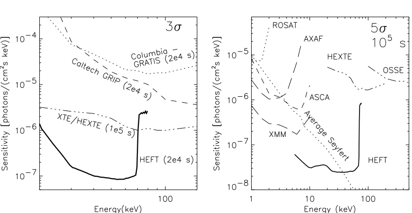
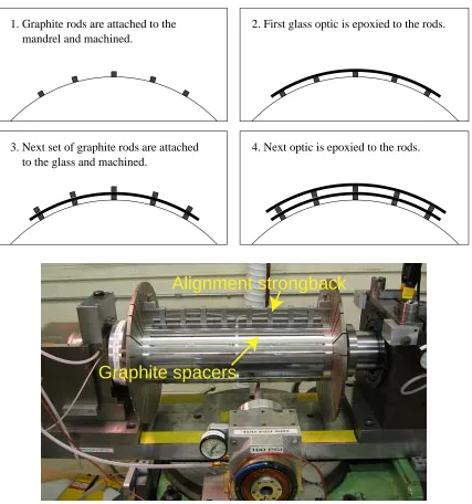
2.1 The sensitivity of HEFT for observations from a balloon platform (left) com-pared to the large-area coded aperture instruments GRIP and GRATIS, and from a satellite platform (right) shown relative to current and future x-ray and gamma-ray instruments. The energy bandwidth is ∆E/E = 50%, and the balloon observations assume an atmospheric column depth of 3.5 g cm−2_{. 8} 2.2 Schematic diagram of the HEFT payload. . . 9 2.3 Top: The HEFT optic mounting and alignment procedure. Bottom: HEFT

uncoated prototype optic on the mounting assembly fixture. . . 13

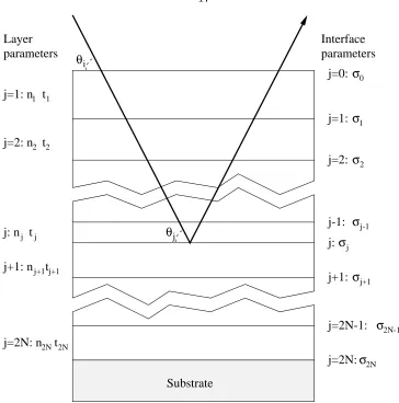
3.1 Schematic diagram of a multilayer coating with notation corresponding to that used in the text. Layers and interfaces are labeled byj,nis the complex index of refraction, t is the layer thickness, and σ is the interface width. Adapted from Joensen, 1995. . . 17 3.2 Calculated reflectivity vs. photon energy at 1.75 mrad of a graded W/Si

multilayer and a Cu/Si multilayer with the exact same specifications (bilayer thickness distribution and interface width). The Cu/Si reflectivity demon-strates that the range in bilayer thicknesses for this mirror would allow re-flectivity at 1.75 milliradian from 20 to 100 keV, but the jump in absorption at the W K-edge (69.5 keV) drastically reduces reflectivity of the W/Si mul-tilayer above the absorption edge. . . 22

4.1 Geometry of conical-approximation Wolter I optics with primary and sec-ondary reflection angles for on- and off-axis rays. . . 26 4.2 Angularly averaged collecting area vs. radial gap between mirror shells.

4.3 Upper left: The two-dimensional reflection angle distribution, Winc(α = 5 mrad, ψ1, ψ2). Because the distribution is nonzero only near the line ψ1=

−ψ2, it is mapped as ψ1+ψ2 vs. ψ1. Each contour line demarcates a factor of ten in the magnitude of the weighting function. Upper right: Projection of the distribution onto the ψ1 +ψ2 axis. One half of the distribution lies within 0.625 µrad of ψ1+ψ2 = 0 and 90% of the distribution lies with 7.5

µrad. Lower left: Projection of the distribution onto theψ1 axis, Winc(α= 5 mrad, ψ1). . . 29 4.4 Figure of merit contour maps of a Joensen parameterized graded multilayer.

The dotted lines represent an N = 200 surface and the solid lines represent anN = 250 surface. The calculations were performed for HEFT’s innermost set of mirror shells. . . 35 4.5 Figure of merit vs. coating thickness for HEFT’sα= 2.32–2.59 mrad mirrors.

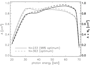
The dashed lines indicate levels of 98% and 95% of the optimum figure of merit. σ is the RMS interface width. . . 39 4.6 Angularly averaged effective area and energy weighted, angularly averaged

effective area (in bold). WE ∝E[keV + 70]. The solid line,N = 233,

corre-sponds to the HEFT design with a figure of merit that is 98% of optimum. The dashed line, N = 363, is our best estimate of optimum design. The fig-ure of merit is the average value of the energy weighted, angularly averaged effective area. . . 40 4.7 Mirror group 4 effective areas at 0.0, 0.5, 1.0, and 1.5 mrad off axis. The

98% optimum design (N = 233) is shown with heavy lines and the optimum design (N = 363) is shown with light lines. . . 41 4.8 Effective area of the full 14-module HEFT design for on-axis sources and

off-axis point sources at 0.5, 1.0, and 1.5 mrad off-axis. . . 42

5.2 Data and model as described in the text for all mirror segments at 34 keV and φ= +5◦. The full line is the model calculation. . . 49 5.3 Data and model as described in the text for all mirror segments at 65 keV

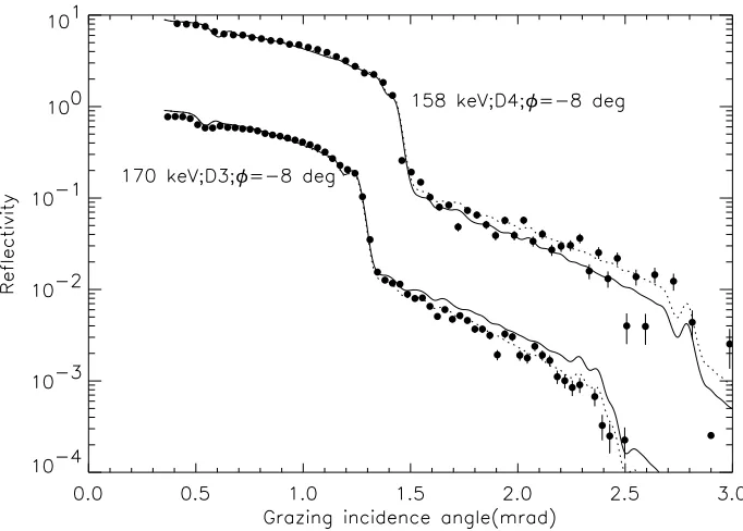
and φ=−8◦. The full line is the model calculation. . . 50 5.4 Data and model as described in the text for mirror segment D3 at 170 keV and

D4 at 158 keV. In both cases, the azimuthal position is φ=−8◦. The solid lines show the calculated reflectivity vs. incidence angle assuming σ= 4.5˚A. The dotted lines are calculated reflectivities forσ = 4.2˚A (D4, 158 keV) and

σ = 4.8˚A (D3, 170 keV). . . 51

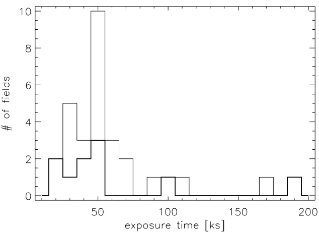
6.1 Exposure time distribution of the SEXSI survey. The heavy line shows the exposure times of the 10 fields for which we have optical spectroscopic data. 53

7.1 ACIS flight focal plane layout. Courtesy of Chandra Science Center [1]. . . 56 7.2 Chandra effective area for front- and back-side chips. Courtesy of Chandra

Science Center [1]. . . 57 7.3 A pathological case demonstrating problems withwavdetect’s determination

of source positions. Left: NGC 1569, chip 2, hard-band CXO image. Data courtesy of Crystal Martin. Right: P60, CCD-13 R band image of the same field. The green circles mark the wavdetect positions. The blue markers indicate centroid positions that do not meet the criteria to supersede the

7.4 More typical source position results fromwavdetect. Here, source c6007 has the largest ∆r2/PSF offset, at 0.21, followed by c6005 with a 0.20 offset. Both are well below our criteria for using centroid-derived positions. Left: HCG 62, chip 6, hard-band CXO image. Data courtesy of Jan Vrtilek. Right: MDM 2.4 m, Eschelle camera R band image of the same field. The green circles mark the wavdetect positions. The blue markers indicate centroid positions. The radii of the markers correspond to the PSF of the mirror array at that location. The north arm of the compass rose is 6000 and the east arm is 3000. . . 59 7.5 ∆r2/PSF vs. wavdetect derived SNR for hard-band detections from NGC

1569, chip 2 and HCG 62, chip 6. The dotted line indicates the cut, above which we adopt the centroid derived position . . . 60

8.1 Example of a low redshift broad line AGN with broad Hαand Hβ lines. The source is a7007 from the 3C 295 field. The permitted Mg and H lines exceed 3800 km/s FWHM. The redshift of the source is 0.4719±0.0009. Here and in the following spectra, the⊕symbol indicates telluric night-sky lines. . . 65 8.2 Example of a broad line AGN from the GRB 010222 field, source b6007. The

redshift of the source is 1.609±0.003. . . 65 8.3 Example of a narrow line AGN from the HCG 62 field, source c7022. The

widths of the permitted emission lines are at resolution limit of the spectro-graph. The redshift of the source is 1.154±0.002. . . 66 8.4 Example of an emission line galaxy from the GRB 000926 field, source b3004.

The red-side flux has been multiplied by 1.4 to compensate for a discepancy in the flux calibration between the red and blue cameras. The redshift of the source is 0.2587±0.0006. . . 66 8.5 Example of an absorption line galaxy from the NGC 1569 field, source d3008.

8.6 Hardness ratio, (H–S)/(H+S), vs. soft (0.5 – 2.1 keV, left panel) and hard (2.1 – 10.0 keV, right panel) band fluxes. The sources are taken from the ten fields for which we have optical spectroscopic data. The vertical scales for both plots are the same; the equivalent photon index scale is shown on the right hand side of the hard-band plot. . . 68 8.7 Top panel: hardness ratio, (H+S)/(H-S), vs. redshift. The right-hand scale

shows the equivalent photon index. The dotted lines trace the hardness ratio vs. redshift of a source with a Γ = 1.7 spectrum, intrinsically obscured by NH column densities of 1020, 1021, 1022, and 1023 cm−1. The solid dots indicate sources with low ratios of soft-band x-ray flux to optical R band flux. Bottom panel: redshift distributions of broad and narrow line AGN, emission line galaxies, and normal galaxies found in the SEXSI survey. . . . 70 8.8 Hardness ratio distributions of broad and narrow line AGN, emission line

galaxies, normal galaxies and optically faint, uncategorized objects. The plots have been slightly shifted to avoid overlapping. On average, emission line galaxies have the hardest x-ray spectra and broad line AGN have the softest spectra. Narrow line AGN and normal galaxies appear to be evenly distributed over the observed -0.6 to 1.0 hardness ratio range. Based on these distributions, the optically faint sources do not appear to be dominated by either broad line AGN or emission line galaxies. . . 71 8.9 Hardness ratio vs. soft-band (left) and hard-band (right) luminosities.

8.10 (a) Soft-band (0.5 – 2.1 keV) and (b) Hard-band (2.1 – 10.0 keV) x-ray to optical (R band) flux ratios vs. the respective x-ray band flux. The dashed lines indicate lines of constant optical flux, at mR = 24 and mR = 25. In general, we do not spectroscopically pursue sources with mR >24. Sources with low soft x-ray to optical flux ratios (< −1.5) are marked with a solid dot. The Ms surveys only observe these sources at soft fluxes below 10−15erg s−1 cm−2. SEXSI, and EMSS before, demonstrate that the optically bright

galaxies are not confined to low soft x-ray fluxes. . . 73

8.11 Fractional contribution of x-ray emission due to star formation vs. star for-mation rate. The SFR is estimated from the [Oii]λ3727 luminosity using Equation 8.1 and the 2–10 keV x-ray luminosity attributed to star formation is calculated from Equation 8.2. The range in the error bars correspond to the range in the conversion factor of Equation 8.2. . . 75

A.1 Mirror group 1: 1.67< α <1.86 . . . 86

A.2 Mirror group 2: 1.86< α <1.86 . . . 87

A.3 Mirror group 3: 2.08< α <2.32 . . . 87

A.4 Mirror group 4: 2.32< α <2.59 . . . 88

A.5 Mirror group 5: 2.59< α <2.89 . . . 88

A.6 Mirror group 6: 2.89< α <3.22 . . . 89

A.7 Mirror group 7: 3.22< α <3.60 . . . 89

A.8 Mirror group 8: 3.60< α <4.01 . . . 90

A.9 Mirror group 9: 4.01< α <4.48 . . . 90

List of Tables

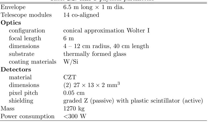
2.1 HEFT performance parameters . . . 9 2.2 HEFT physical parameters . . . 10

3.1 Comparison of the physical properties of a few multilayer material combina-tions [2]. Absorption coefficients are given for 30 keV x-rays. . . 23

4.1 HEFTdesign: mirror groups and bilayer thickness specifications. . . 37 4.2 Comparison of multilayer performance limits (idealized case vs. HEFT

pa-rameters). Column 3 (θmax): maximum reflection angle at the maximum photon energy. Column 4 (Emax): maximum on-axis reflected energy on the outermost shell within each group, disregarding absorption edge effects. Col-umn 5: estimated fractional loss in 70 keV effective effective area for sources at the edge of the field of view. . . 38 4.3 HEFTdesign parameters for W/Si. . . 43

5.1 HEFTprototype design parameter. . . 48 5.2 Minimum bilayer thickness [˚A] determined by hard x-ray measurements

con-ducted at ESRF. . . 50

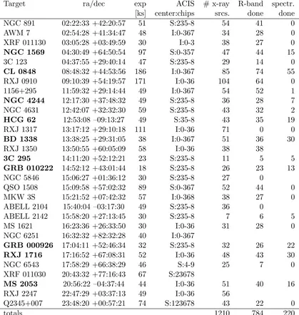
6.1 Status of optical spectroscopy follow-up observations. . . 54

Chapter 1

Introduction

The research described in this thesis is rooted in the effort to investigate astronomical x-ray emission at higher energies and to fainter flux levels than previous missions have been capable of. The first part of this thesis covers the design and fabrication of the optics for a hard x-ray telescope, the High Energy Focusing Telescope (HEFT), one of the first telescopes to focus x-rays at energies above 20 keV. Observations in the hard x-ray band (10–100 keV) will allow us to study nonthermal emission processes that are not accessible at low energies and sources whose low energy emission is obscured by intervening dust or gas. For technical reasons, hard x-ray telescopes have not previously been capable of achieving the required sensitivity levels. The development of HEFT is one of the first efforts to employ focusing technology in order to dramatically improve the sensitivity of hard x-ray telescopes. The second part of the thesis presents the preliminary results of the Serendipitous Extragalactic X-ray Source Identification (SEXSI) survey, a square-degree scale survey of sources detected in the 2–7 keV band with the Chandra X-ray Observatory. Although Chandra is only sensitive below 10 keV, its faint flux sensitivity limit is orders of magnitude better than that of prior missions, allowing us to observe previously inaccessible sources.

popula-tion of electrons. By combining the two measurements, one can determine the strength of the magnetic field in the galaxy or cluster. In most cases, the x-ray measurement is nearly impossible at low energies because thermal emission dominates the x-ray spectrum below 10 keV.

Another impetus to improve hard x-ray sensitivity is the ability to detect sources that are obscured at lower energies. Column densities between 1020and 1025 atoms/cm2 impact our ability to detect sources in the x-rays.1 At 1020 cm−2, which is a typical value of the galactic column density at high galactic latitudes, there is no appreciable attenuation of x-rays down to 0.5 keV. Above 1025cm−2, obscuring material is considered Compton thick: hard x-rays (E _∼>10 keV) are converted into soft x-rays via Compton scattering which are then photoelectrically absorbed. Column densities between those two extremes limit the ability of a given instrument to detect sources. For example, ROSAT, which operated in the 0.1–2.5 keV range and performed the last x-ray all-sky survey, was unable to detect sources behind absorbing columns greater than 1022 cm−2. The most sensitive x-ray telescopes in operation today, Chandra and XMM-Newton, detect x-rays up to approximately 8–10 keV. An absorbing column of 1024 cm−2 would block the < 10 keV emission from all but the most luminous sources. A high-sensitivity, hard x-ray telescope would allow us to study obscured x-ray sources out to the Compton-thick limit.

High-sensitivity, hard x-ray observations of the x-ray sky have not yet been carried out because the imaging systems currently in use, collimators and coded aperture masks, cannot reach the required sensitivity levels. Focusing telescopes have provided high-sensitivity observations at low energies, E <10 keV, but were restricted to low energies by technical limitations. The present generation of astronomical instruments operating in the hard x-rays employ either coded aperture masks (Integral) or collimators (RXTE) to detect x-ray sources. The noise in x-ray measurements is dominated by the internal detector background rate, so the minimum detectable flux is proportional to the ratio of the detecting area to the effective collecting area (Adet/Aeff). With a collimator, Adet/Aeff ≈1, and with a coded aperture mask, the ratio of the areas rises to 2:1. Coded aperture systems, despite their obvious sensitivity limitation, still have a place in x-ray astronomy because of their ability to perform wide field-of-view imaging. The faint source sensitivity of focusing systems is

1

much better than that of collimator and coded mask systems because the detecting area of a focuser is orders of magnitude smaller than its collecting area. The use of focusing in the low energy x-ray band began with the Einstein Observatory (1978 - 1981, 0.1–4 keV). With a ratio of detecting to collecting area of 103 – 104, the Einstein Observatory was hundreds of times more sensitive than its nonfocusing predecessors. The energy range of focusing telescopes has been extended to∼10 keV with the Chandra X-ray Observatory (CXO) and XMM-Newton, both launched in 1999. CXO, with arcsecond imaging performance has a collecting to detecting area ratio of roughly 107.

Focusing optics have not been used at energies above 10 keV because the optics currently used on x-ray telescopes are difficult to employ in practical hard x-ray telescopes. Today’s focusing telescopes rely on total external reflection. In the x-rays, where the refractive indices of materials are smaller than the vacuum refractive index, total external reflection occurs at grazing incidence angles, on the order of several milliradians. The grazing inci-dence optics used by Chandra, XMM and all previous x-ray focusing telescopes are difficult to use at higher energies because the critical reflection angle, above which reflectance is negligible, is roughly proportional to 1/E. The main problem with total external reflec-tion grazing incidence optics is that the reducreflec-tion in the critical angle at higher energies translates directly into a decrease in the field of view of the telescope. In addition, the small graze angles force the telescope design to employ either small radius optics or a long focal length. Small radius optics are undesirable because they dilute the sensitivity gains of focusing systems. A long focal length (>30 m) increases the power (and hence weight and cost) requirements on the spacecraft for pointing.

Goddard Space Flight Center and Nagoya University in Japan, and the High Energy Fo-cusing Telescope (HEFT) [7, 8], being developed by Caltech, Columbia University, Danish Space Research Institute, and Lawrence Livermore National Laboratory. In addition, the Constellation-X mission concept [9] includes a hard x-ray focusing telescope.

One of the major scientific motives for developing hard x-ray focusing telescopes is to trace the history of accretion from the formation of the first structures to the present epoch and to determine the fraction of accretion power obscured at lower energies by large absorption columns. The rapid time variability (days or shorter) of x-ray emission from active galactic nuclei (AGN) implies that x-rays are generated in a small region [10]. The power per unit volume of the x-ray emitting region in active galaxies can only be explained by the accretion of matter onto a super-massive black hole. In the local universe and at low energies, AGN are the dominant source of extragalactic x-radiation [11, 12]. Furthermore, most models of the extragalactic x-ray background (XRB) predict that AGN are responsible for practically all of the flux [13, 14, 15, 16]. We know that the power released by accretion and the environment in which it occurs has evolved over time because the spectrum of the XRB cannot be reproduced by the integrated spectra of nearby, bright x-ray sources [17] and because QSOs have undergone significant evolution. XRB synthesis models use AGN redshift and obscuration column distributions to reproduce the observed background spectrum. These models predict that a significant fraction of the hard XRB comes from sources that are totally obscured in the soft x-rays [18]. Most of the power in the XRB spectrum is concentrated in the 20–40 keV band, so developing high-sensitivity instruments for that energy range is necessary to develop a comprehensive understanding of the accretion history of the universe.

have found that at these higher energies, a smaller fraction of the spectroscopically classi-fied sources, roughly 1/2, exhibit AGN signatures [20, 21]. The SEXSI survey, which uses 40–100 ks Chandra observations, complements the deep, megasecond surveys by covering a much larger area of the sky. Although SEXSI does not reach the flux levels of the deep surveys by a factor of ten, it covers approximately thirty times the area. The SEXSI survey allows us to address issues of field-to-field variations, especially at the bright source end (10−15 – 10−14 erg cm−2 s−1, 2–10 keV), where the statistics of the deep surveys will be poor.

A combination of wide field of view (FOV) survey instruments and high-sensitivity focusing telescopes will be required to study the heavily obscured sources that are expected to be responsible for the hard XRB. At the flux sensitivity level achievable in the next decade, the density of hard x-ray sources will still be too low for deep field surveys to produce meaningful results. We first need wide FOV instruments conducting all-sky surveys to locate the hard x-ray sources. We then need focusing instruments to provide accurate positioning and high-sensitivity spectroscopy of the cataloged sources. The last all-sky survey in the hard x-rays was completed more than 20 years ago using the collimated A4 instrument on HEAO 1 and reached a sensitivity limit of ∼ 13 mCrab(2) [23]. New hard x-ray all-sky surveys will be performed in the next few years with the coded aperture mask instruments on the INTEGRAL and Swift missions. Coded aperture masks are well suited for large area surveys because of they can be designed with wide fields of view; however, they have poor angular resolution (relative to focusing telescopes), typically on the order of 100. The Burst Alert Telescope (BAT), a coded mask instrument on Swift, is designed to detectγ-ray bursts, but it will also conduct an all-sky survey over the 10–100 keV range to a sensitivity limit of ∼1 mCrab. BAT expects to discover 400–600 hard x-ray sources in its all-sky survey, but the energy resolution and sensitivity of the instrument will be insufficient for detailed spectroscopic analysis. Furthermore, its point spread function (170) is too large to reliably cross identify the sources in longer wavelength bands for follow up observations. Focusing telescopes, such as HEFT and Constellation-X, will be used to perform follow up observations of the Swift catalog sources. Although the field of view of a focusing telescope is much smaller than that of a coded mask instrument, focusing telescopes provide far superior angular resolution. HEFT and Constellation-X follow-up observations

will improve the astrometric positions of the hard sources to sub-arcminute levels. In addition, the higher sensitivity and finer energy resolution of the focusing instruments will allow us to measure the x-ray spectra of the Swift sources. The new wide field instruments and focusing telescopes operating in the hard x-ray band will provide strong observational constraints on the XRB synthesis models.

Chapter 2

Overview of the High Energy Focusing Telescope

HEFT will be among the first astronomical instruments to focus x-rays at energies above 20 keV. The impressive gain in sensitivity achievable with focusing is illustrated in Figure 2.1. As a balloon-borne instrument, HEFT will be sensitive to sources two orders of magnitude fainter than those detected by the coded aperture mask instruments GRIP and GRATIS (both also flown on balloons). The potential of a satellite-borne focusing telescope is shown in the right panel of Figure 2.1. The ability to take long exposures and the absence of atmospheric attenuation would give HEFT almost three orders of magnitude better sensi-tivity than the collimated High Energy X-ray Timing Experiment (HEXTE) on board the Rossi X-ray Timing Explorer, presently the highest sensitivity instrument in the 20-100 keV band. The improved sensitivity will give us a more comprehensive view of the hard x-ray sky, allowing us to study nonthermal processes in a variety of astrophysical sources. In addition to gains in faint source sensitivity, HEFT will have the best angular resolution,

∼10(0.3 mrad) half energy width (HEW), and will be one of the highest spectral resolution instruments,<1 keV FWHM at 60 keV, ever operated in the 20 – 70 keV band.

As one of its main objectives, HEFT will be used to conduct a spectroscopic survey of mCrab flux AGN. Initially, we will select sources from low energy x-ray catalogs (ROSAT and Einstein) but these catalogs will select for unobscured, type 1 AGN. The obscured, type 2 AGN population is much more interesting because they are thought to contribute to the bulk of the XRB at high energies. Presently, the only comprehensive catalog of hard x-ray sources is the HEAO 1 A-4 catalog, which covers the 13–180 keV band to a flux level of

∼13 mCrab [23]. The HEAO 1 A-4 catalog finds only five active galaxies, all of which have been extensively studied in the intervening years. The Swift mission will conduct a mCrab sensitivity survey over the 10–100 keV range and is predicted to locate approximately 400 sources, with the majority being obscured at lower energies [24]. HEFT’s 3σ continuum sensitivity limit is less than 0.1 mCrab, so our follow-up of the Swift detections will produce high-quality spectra of several type 2 AGN.

Figure 2.1: The sensitivity of HEFT for observations from a balloon platform (left) com-pared to the large-area coded aperture instruments GRIP and GRATIS, and from a satellite platform (right) shown relative to current and future x-ray and gamma-ray instruments. The energy bandwidth is ∆E/E = 50%, and the balloon observations assume an atmospheric column depth of 3.5 g cm−2.

remnants, HEFT will detect the 68 keV emission resulting from the decay of 44Ti, an element created near interface between ejecta and in-fall material in supernova explosions [25]. The energy resolution of the HEFT’s cadmium-zinc-telluride (CZT) detectors will allow us to resolve Doppler broadening of the 68 keV emission line. HEFT will map the44Ti distribution of the Cas-A remnant in three dimensions, providing observational constraints on supernova nucleosynthesis models. In clusters of galaxies, the magnetic field can be determined by combining radio synchrotron and x-ray inverse Compton measurements. The inverse Compton flux results from microwave background photons scattering off the relativistic electrons that produce the radio emission. The inverse Compton flux has a power law spectrum, in contrast to the thermal bremsstrahlung spectrum which falls away at high energies. With HEFT, we will look for a deviation from the thermal bremsstrahlung spectrum in the diffuse emission of Coma and other clusters of galaxies.

2.1

Payload overview

telescopes. Each telescope consists of a conical approximation Wolter 1 optics module and an actively shielded cadmium-zinc-telluride (CZT) detector. The telescope will be sensitive over the 20–70 keV energy range, limited at the low end by atmospheric absorption and at the high end by the choice of multilayer material. A schematic of the telescope is shown in Figure 2.2. The performance parameters are listed in Table 2.1 and the physical parameters are listed in Table 2.2.

Figure 2.2: Schematic diagram of the HEFT payload.

Table 2.1: HEFT performance parameters Bandpass 20 – 69.5 keV

Effective area 300 cm2 at 30 – 40 keV Energy resolution <1 keV FWHM at 60 keV Angular resolution 0.3 mrad (10) HEW on-axis Field of view 3.0 mrad FWHM in area

2.1.1 Detectors

Cadmium-zinc-telluride is a semiconductor ideal for use in the hard x- and softγ-ray bands. Its bandgap (1.57 eV) is large enough so that, unlike germanium detectors, it may be used without cryogenic cooling. The average atomic number of CZT’s constituent elements results in a relatively large cross section to high energy x-rays. A 2 mm thick CZT crystal will have quantum efficiency close to 100% up to 100 keV. For comparison, a silicon detector of the same thickness is only efficient up to∼20 keV.

Table 2.2: HEFT physical parameters

dimensions 4 – 12 cm radius, 40 cm length substrate thermally formed glass

shielding graded Z (passive) with plastic scintillator (active)

Mass 1270 kg

Power consumption <300 W

plastic scintillator is used in anticoincidence with the detector to reduce background from spallation products. The detector is further shielded from secondary x-rays by a series of lead, tin and copper sleeves lining the inside wall of the plastic shield.

The pixel pitch of the detectors, 0.05 cm, oversamples the projected angular resolution of the optics by a factor of 3. Each detector is indium bump-bonded to a VLSI chip with separate event triggering, preamplification, and pulse sampling circuitry under each pixel. This arrangement minimizes stray capacitance between the detector and the preamplifi-cation stage, significantly reducing electronic noise in the detector electronics. The latest tests of the detector/VLSI hybrid indicate that HEFT’s spectral resolution should fall in the range 0.5 – 1.0 keV FWHM at 60 keV. For more details on the detectors see Harrison

et al. (2000) [26] and references therein.

2.1.2 Optics

m focal length, the primary opening angles will range from 1.67–5.0 mrad. Each telescope module will consist of 72 nested mirror shells filling roughly 50% of the aperture. More details on the shell packing arrangement and its optimization are discussed in Section 4.1. The tight packing arrangement of HEFT’s optics requires that we use a mirror substrate that is thin, stiff and light. The Wolter I geometry requires that the substrate be easily formed into conical sections. Finally, in order to maximize the performance of the coatings, the substrate must have relatively low (< 4˚A) surface roughness. D263, a borosilicate glass produced by the DESAG division of Schott, meets the requirements for the HEFT optics. D263 is manufactured in a “down-draw” process where the glass is formed by flowing through a slot in the bottom of the melting tank. This manufacturing process can produce glass in thickness ranging from 30–1100µm with RMS surface roughness typically less than 4 ˚A. HEFT will use 200 and 300 µm thick D263, thermally formed [8] and then cut into 10 cm long, 45◦ cylindrical sections. The glass is thin and flexible enough to allow the mounting process to force the cylindrical glass sections into the conical configuration required for focusing. X-ray reflectance tests comparing multilayer coatings on flat and slumped glass showed that the slumping process did not adversely affect the surface quality of the glass [7].

Two other common substrate materials for hard x-ray optics are epoxy-replicated alu-minum foils (ERAFs) and electroformed nickel shells. We considered ERAFs for HEFT but in the end decided that the production process would require too many sensitive steps and that glass would provide equivalent to superior performance with much simpler production methods. Electroformed nickel is attractive because it can be used to produce full-revolution true Wolter I optics; however, it is prohibitively costly, requiring a separate mandrel for each radius optic, and nickel shells would be much heavier than glass shells.

mandrel and machined.

2. First glass optic is epoxied to the rods.

to the glass and machined.

4. Next optic is epoxied to the rods. 1. Graphite rods are attached to the

3. Next set of graphite rods are attached

Alignment strongback

Graphite spacers

Chapter 3

Principles of x-ray multilayers

X-ray focusing can be achieved either through reflection or refraction. In the x-ray band, the real part of the refractive index for all materials is less than the vacuum refractive index by a very small amount (10−3_–10−6 _{at 10 keV). Consequently, reflective optics must} operate at grazing incidence angles where a condition for total external reflection exists. Refractive optics must use compound lenses to shorten the focal length to a usable distance [27]. Refractive optics must have surfaces with small radius of curvature, so they are best suited to situations where small apertures are acceptable. Also, because the refraction angle, and hence the focal length, is energy dependent, refractive lenses are not suitable for broad band applications. Grazing incidence reflective optics are the standard choice for x-ray astronomy, where large apertures and energy independent focal length are important. This chapter covers the basic physics of x-ray reflection from standard materials and multilayer coatings. Multilayer coatings are considerably more complex than single-material reflectors, so some multilayer design considerations and material selection criteria will also be discussed.

3.1

X-ray reflection from standard materials

Standard materials, especially high Z elements, make highly efficient x-ray reflectors at grazing incidence angles where a condition for total external reflection exists. Conversely, at larger incidence angles, outside of the total external reflection regime, the reflectance rapidly falls off to virtually unusable values. The energy dependence of the critical angle for total external reflection limits the practical use of standard reflectors in astronomical telescopes to low energies (E_∼<15 keV).

The x-ray index of refraction, nr, of materials is often written as

nr= 1− N reλ2

2π (f1+if2) = 1−δ−iβ, (3.1)

where N is the number density of atoms, re is the classical electron radius, λ is the

is related to the absorption cross section (µa) and the transmission coefficient (T) by the

The real part ofnr is used by Snell’s law to calculate the refraction angle. Becausenrin

the x-rays is less than the refractive index in vacuum, x-rays exhibit total external reflection at small grazing incidence angles. The maximum grazing incidence angle, or critical angle (θc), is related to the refractive index by Snell’s law:

cos(θc) =nr. (3.4)

The relationship between photon energy and critical angle is found by combining Equations 3.1 and 3.4:

Since λ = hc/E, it is often stated that the critical angle is inversely proportional to the incident photon energy. Although the form factor, f1, is also dependent on energy, its dependence is weak. The form factor is the measure of the number of “free” electrons in the system, i.e., the number of electrons whose binding energy is less than the photon energy, so at energies greater than a few keV and away from photoelectric transitions,f1 is nearly constant. In the following discussion, I will use the symbolρe =N f1 as the effective electron density.

The reflectance function, R, of a standard (nonstratified) material is calculated from the Fresnel formulae (see Born and Wolf 1980 for derivation):

rT E = sinθi−nsinθt

where n is the complex refractive index of the material, θi is the grazing incidence angle

related to θi by Snell’s law. For unpolarized light, the reflectivity function is:

Whenθi < θc, the angle of transmission,θt, is imaginary, causing the terms in the numerator

of Equations 3.6 and 3.7 to be out of phase in the complex plane, resulting in Fresnel coefficients with magnitude near 1. When θi > θc, then θt is real and because δ << 1, θi ≈θt, so the Fresnel coefficients are nearly zero. With the exception of Bragg reflection

off of crystalline solids, the x-ray reflectivity of standard materials is negligible at incidence angles greater than the critical angle.

3.2

X-ray reflectivity from multilayers

In order to achieve appreciable x-ray reflectivity at incidence angles greater than θc, one

can use thin film coatings to create a synthetic Bragg crystal. Such thin film coatings are commonly referred to as “multilayers” [4, 5]. In order to be effective at reflecting x-rays, multilayers are deposited as alternating layers of high and low refractive index materials (e.g., tungsten and silicon (W/Si), or platinum and carbon (Pt/C)). Figure 3.1 illustrates a generic multilayer coating. Typical values for the layer thicknesses range from 10–100˚A with total coating thicknesses up to a few microns.

The reflectance function of a multilayer coating can be calculated via recursive appli-cation of the Fresnel formulae to the reflectivity calculation for a single film. The Fresnel reflection coefficients for the jth interface are

r_jT E = njsinθj−nj+1sinθj+1

used to calculateθj, the refracted angle of the transmitted beam. Because we are considering

θj

Figure 3.1: Schematic diagram of a multilayer coating with notation corresponding to that used in the text. Layers and interfaces are labeled byj,nis the complex index of refraction,

tis the layer thickness, and σ is the interface width. Adapted from Joensen, 1995.

algebraically equivalent form of Snell’s law:

njsinθj =

q

n2_j + sin2θi−1. (3.11)

The reflectivity of the coating,R, is found by recursively calculating the reflection coefficient for a single thin film:

r_≥j =

rj+r≥j+1exp(−i2φj+1) 1 +rjr≥j+1exp(−i2φj+1)

, (3.12)

wherer_≥j is the combined reflection coefficient for interfacesj . . .2N and φj is the change

in phase of the radiation as it passes through layer j with thicknesstj:

φj =

2π

The recursion relation starts at the j = 2Nth interface with r_≥2N = r2N. It is safe to

assume that r2N+1, the reflection coefficient for the back side of the substrate, is zero as long as the substrate is much thicker than the coating. The recursion ends atj= 0 and we find the reflectivity of the coating:

R=|r_≥0 |2 . (3.14)

The Fresnel formulae give us the reflectance function of a multilayer coating with perfect interfaces. In practice, print-through of substrate roughness, deposited thin film roughness, and interdiffusion between adjacent layers conspire to reduce reflectivity from the ideal case. Roughness and interdiffusion are taken into account by multiplying the Fresnel coefficients (r_≥j) by the N´evot-Croce factor [28]:

The N´evot-Croce factor is essentially the Debye-Waller factor with refraction taken into account.

3.3

General design considerations

3.3.1 Bilayer thickness range

The bilayer thickness, d, (or thicknesses, dk) of a multilayer coating is equivalent to the

lattice spacing of a crystal when one considers its Bragg reflection properties. The Bragg formula, mλ = 2dsinθ (where m is an integer), is used to estimate (or calculate) the bilayer thicknesses to be used in any particular application. For completeness, the refraction corrected Bragg formula and its derivation are outlined here, but in practice, the standard formula is used more often.

derive the refraction-corrected Bragg formula [29]:

By inverting the first-order (m= 1) Bragg equation for d, one can estimate the range in bilayer thicknesses required to enhance reflectance over the energy range Emin−Emax and angular range θmin−θmax:

For the minimum bilayer thickness, we can drop the refraction-correction term because typicallyθmaxθc. The maximum bilayer thickness, however, requires more careful

atten-tion because specificaatten-tions (including those for HEFT) may result in a substantial refracatten-tion correction. When θmin ≈ θc, the standard Bragg formula for crystals underestimates the

maximum bilayer thickness.

3.3.2 Bilayer thickness distribution

Broadband reflectivity is achieved with multilayer coatings by varying the bilayer thick-nesses throughout the coating. Lateral gradations are used in some specialized thermal neutron beam or synchrotron applications, but for astronomical x-ray telescopes, depth graded multilayer coatings are the norm. The Bragg formulas, Equations 3.17 and 3.18, give the required range in bilayer thicknesses for a given application, but the distribution of bilayer thicknesses still must be specified. Methods for specifying the bilayer thickness dis-tribution generally fall into two categories: power-law disdis-tributions and “needle variation” derived distributions.

coefficients scale as ∆ρe/E2. Ignoring attenuation and scattering due to roughness, this

implies that each factor of 2 in energy requires 24times as many bilayers in order to achieve a flat response.

The use of power-law bilayer thickness distributions originated with F. Mezei (1976) [30], who was also the first to propose the use of multilayer coatings for the reflection of thermal neutrons. Mezei’s approach to power-law parameterization is outlined in Joensen (1995) [31] and will not be repeated here. Mezei (1976) derives a power-law formula for flat response, broadband neutron mirrors assuming thatN, the number of bilayers, is large and ignoring multiple reflections and absorption/extinction. The Mezei formula is

d(k) =dc/k0.25, (3.19)

where k is the index of the bilayer consisting of layers j = 2k−1 and j = 2k, and dc = λ/2 sinθc. Note also that his definition for the maximum bilayer thickness (dc) does not

include any refraction corrections to the Bragg formula.

Other power-law parameterizations have been developed [32, 33, 34] but will not be expanded upon, with the exception of Joensen’s parameterization. In his thesis, Joensen proposes an empirical distribution formula which is a generalization of the Mezei formula:

d(k) = a

(b+k)c (3.20)

witha, c >0 andb >−1. Using the energy weighted average reflectance at a single incidence angle as his figure of merit, Joensen finds superior performance with his parameterization when compared against those of Mezei (1976), Schelten and Mika (1978), Hayter and Mook (1989), and Yamada et al. (1978). For this reason, Joensen’s parameterization is used in the optimization of the HEFT multilayer design.

work of Kozhevnikov et al. (1998, 2001) [37, 38], a recursion relation has been developed to calculate an initial distribution for a given reflectance profile. Standard minimization techniques (Newton-Raphson, Levenberg-Marquadt, simplex) are then used to minimize the mean square difference between the calculated reflectance and the desired profile. The limitation to Kozhevnikov’s present method is that the number of bilayers is fixed, narrowing the search space considerably, but also, very likely, missing the true optimal design. It is possible that the needle variation technique, in conjunction with Kozhevnikov’s recursion relation, would be a very powerful technique for solving the “inverse problem.”

3.4

Multilayer materials

In choosing material combinations for a graded multilayer one must consider that the band-pass and the reflectivity are limited by attenuation in the multilayer coating because of photoelectric absorption and scattering at the interfaces. The ideal material pairs have a large difference in refractive index; minimal absorption over the energy range of interest; and can be fabricated with sharp, smooth interfaces.

The Fresnel formulae (Equations 3.9 and 3.10) show that the reflectance of an interface scales with the difference in refractive index between the two sides of the interface. As previously discussed, δ ∝ ρe and since the effective electron density is proportional to

the mass density, one can use bulk density as an initial screen to find promising pairs of materials for multilayers. At the energies of interest (10-100 keV), photoelectric absorption is the main component of an atom’s cross section and, away from absorption edges, it scales roughly as Z4E−5/2. Highly absorbing materials are to be avoided because the reflectance of a multilayer made with such materials levels off with fewer bilayers than that of a coating using smaller cross section materials. Thus, if the reflectivity per interface is the same, the material combination with a lower absorption coefficient will have better reflectance.

Figure 3.2: Calculated reflectivity vs. photon energy at 1.75 mrad of a graded W/Si mul-tilayer and a Cu/Si mulmul-tilayer with the exact same specifications (bilayer thickness distri-bution and interface width). The Cu/Si reflectivity demonstrates that the range in bilayer thicknesses for this mirror would allow reflectivity at 1.75 milliradian from 20 to 100 keV, but the jump in absorption at the W K-edge (69.5 keV) drastically reduces reflectivity of the W/Si multilayer above the absorption edge.

Following the selection of materials based on refractive index contrast and minimal ab-sorption, one must experimentally determine which material combinations are compatible. Problems that may arise include excessive interdiffusion, which reduces the refractive index contrast, high levels of stress in the film, which may result in delamination, and corrosion. Other experimentally determined factors include maximum deposition rates of the materials and deposited surface roughness.

Table 3.1: Comparison of the physical properties of a few multilayer material combinations [2]. Absorption coefficients are given for 30 keV x-rays.

materials ρ1/ρ2 µ11 µ22 [cm−1] [cm−1]

Pt/C 9.77 566. 0.435

W/Si 8.28 439. 3.35

Mo/Si 4.38 287. 3.35

Ni/C 4.05 92.0 0.435

Chapter 4

Optimization of multilayer designs

The current literature on multilayer optimization almost exclusively deals with maximizing integrated reflectance [39, 40] or matching the reflectance to a desired function [39, 37, 41] either over a range of photon energies at a single reflection angle or over a range or reflection angles at a single photon energy. Optimization methods that optimize a multilayer design for a single angle or a single photon energy may be useful for laboratory applications where reflection angles and/or photon energies are fixed. For a general-purpose astronomical hard x-ray telescope, however, maximizing the effective area over a given energy range and field of view (i.e., a relatively wide range of incidence angles) is more important than producing a specific response at a single energy or reflection angle. For example, galaxy clusters and nearby radio galaxies are extended at the few arcminute level. In addition, for a balloon-borne instrument, one must account for instabilities in the pointing of the telescope which can also be at the few arcminute level. For these reasons, the off-axis performance of astronomical x-ray telescopes deserves at least as much attention as the often-quoted on-axis performance.

To this end, I devised a figure of merit function that is the field-of-view and energy-weighted average effective area of a telescope’s optics [42]. The calculation of the figure of merit requires specification of the geometry of the telescope optics, weighting functions for spectral and angular response and the matrix of multilayer reflectivity vs. energy and incidence angle.

4.1

Geometry of the optics

used in the ray trace affects the optimization of the geometry of the optics and determines the reflection angle distributions that will be used to calculate the figure of merit. I use a uniform distribution of off-axis angles between 0 and 3 mrad, with the largest angle set by the size of our detectors and the focal length of the telescope. To design geometries and multilayers with greater off-axis performance (at the expense of on-axis performance), one would use an input distribution that favors off-axis photons.

HEFT’s optics are arranged in a conical approximation to the Wolter I (parabola/ hyperbola) geometry. HEFT uses thermally slumped glass which presently has figure errors that result in a point spread function at the 10 level. A schematic of the optics’ geometry and the relevant angles are shown in Figure 4.1. The half-opening angles of the mirror shells are set by the following equations:

αi =ri/(4f) (4.1)

βi = 3αi, (4.2)

whereαi andβi are the respective half-opening angles of the primary and secondary shells, ri is the radius of the ith shell at the plane between the primary and secondary mirror

sections (4–12 cm for HEFT), and f is the focal length of the telescope (6 m for HEFT). The HEFT substrates are 0.3 mm thick, 20 cm long sheets of Schott DESAG D263 glass.

The difference in radii between consecutive concentric mirror shells produces a tradeoff between on- and off-axis collecting areas. On-axis collecting area is maximized when the inner radius of the i+ 1st primary shell lies on the same coaxial cylinder as the outer edge of theith primary shell. Increasing the radial gap (cf Figure 4.1) between consecutive shells improves off-axis collecting area at the expense of on- and nearly on-axis area. I explored two methods of defining the extra gap between mirror shells: a constant gap between all shells, such that the difference in radii between consecutive shells is

∆ri,i+1=αil+ const., (4.3)

wherelis the length of the mirror along the optical axis, and a radius dependent gap where the gap between the consecutive shells is

Figure 4.1: Geometry of conical-approximation Wolter I optics with primary and secondary reflection angles for on- and off-axis rays.

where ξ is the variable gap parameter. When ξ = 0, there is no additional gap between shells; whenξ= 1, the gap is equal to the projected radial width of the primary shell. From ray tracing with perfect reflectivity,R= 1, one finds that the angularly averaged collecting area (the fraction of collected events multiplied by the illuminated area) is maximized with a constant gap of 0.17 mm between consecutive shells (see Figure 4.2). A variable gap with

ξ= 0.26 maximizes the area for that method, but falls short of the constant gap geometry by a fraction of a percent.

4.2

Effective areas

Figure 4.2: Angularly averaged collecting area vs. radial gap between mirror shells. Variable gap results (+) are plotted against the bottom scale and constant gap results (×) are plotted against the top scale. Each area is determined by ray tracing 108 events uniformly distributed in off-axis angles between 0 and 3 mrad, and uniformly distributed spatially over the 12 cm radius aperture. The standard deviation in the estimate of the area is 0.025 cm2.

4.2.1 Geometry-dependent area

The physical collecting area and the mirror reflectance function are the the two components of the geometry-dependent part of the effective area. On-axis effective area is easy to calculate, since the incidence angles on the primary and secondary mirrors are identical. The area of the ith shell is thus

Ai(E) = (2πriαil)·([R(E, αi)]2), (4.5)

wherelis the length of the mirror along the optical axis andE is the energy of the photon. The first term in the above equation is the projected area of the primary mirror, and the second term gives the reflection efficiency.

from a source at off-axis angleψ. The incidence angles on the primary and secondary mirrors are θ1 =α+ψ1 and θ2=α+ψ2, respectively. The angles ψ1 and ψ2 have values between

−ψ andψ, depending on the difference between the azimuthal angle of the source and the azimuthal position of the point of reflection, ∆φ. For example, when ∆φ = 0, ψ1 = −ψ and when ∆φ=π, ψ1 =ψ. With conical approximation Wolter I optics with α 1, one can make the approximation that ψ1 = −ψ2. This approximation allows one to calculate the effective area using only the incidence angle distribution on the primary mirrors. The one-dimensional function Winc(αi, ψ1) is the incidence angle distribution generated by the ray trace with off-axis angles uniformly distributed between 0 and 3 mrad. Winc has units of area and is related to the event distribution (the raw output of the ray trace) by the density (events/unit area) of input events. The angularly weighted effective area is

Ai(E) =

Z _ψ

−ψ

dψ1Winc(αi, ψ1)·[R(E, αi+ψ1)R(E, αi−ψ1)] (4.6)

where ψ is the half angle of the full field of view. There is no explicit integration in the azimuthal (φ) direction in Equation 4.6 because it is already incorporated into the distribution function by the ray trace.

If one cannot use the approximation ψ1 = −ψ2, then it is necessary to explicitly keep track of the correlation between ψ1 and ψ2 in the ray trace and generate a two-dimensional incidence angle distribution for each set of mirror shells. A contour map of the two-dimensional incidence angle distribution for HEFT’s the outermost set of mirrors and associated projections are shown in Figure 4.3. The sum of the deviation angles, ψ1+ψ2, is used instead of ψ2 alone on the y-axis and the contours denote logarithmic intervals. The Figure 4.3 demonstrates the excellent degree to which the ψ1 =−ψ2approximation is valid for conical approximation Wolter I optics. Note that the y axis scale is in microradians, whereas thexaxis scale is in milliradians. With a two-dimensional distribution, the angu-larly weighted effective area is

extending the technique to geometries with even more reflections is trivial: one simply adds one dimension to the incidence angle distribution matrix for each additional reflection.

Figure 4.3: Upper left: The two-dimensional reflection angle distribution, Winc(α = 5 mrad, ψ1, ψ2). Because the distribution is nonzero only near the line ψ1 = −ψ2, it is mapped asψ1+ψ2 vs. ψ1. Each contour line demarcates a factor of ten in the magnitude of the weighting function. Upper right: Projection of the distribution onto the ψ1+ψ2 axis. One half of the distribution lies within 0.625 µrad of ψ1+ψ2 = 0 and 90% of the distribution lies with 7.5µrad. Lower left: Projection of the distribution onto theψ1 axis,

Winc(α= 5 mrad, ψ1).

4.2.2 Transmission components of the effective area

the detectors, and, most importantly, the atmosphere above the telescope. HEFT uses CZT detectors and in the energy range of interest, the QE of CZT is not a strong function of photon energy.

The transmission function for atmospheric attenuation is defined as

Tatm(E, ρatm) = exp(−η(E)ρatm), (4.8)

where η(E) is the attenuation coefficient of dry air and ρatm is the altitude dependent atmospheric column density. The area is thus redefined:

˜

A(E, ρatm) =A(E)Tatm(E, ρatm). (4.9)

For HEFT, we assume a column density of 3.5 g/cm2_{, corresponding to an altitude of 39} km.

At this time the thicknesses of the kevlar pressure vessel and the mylar windows on the mirrors have not been decided upon; however, the transmission functions of these windows are expected to be close to unity at energies above 20 keV. Consequently, their omission will not significantly change the results of the optimization.

4.3

Figure of merit function

We use the angularly weighted effective area to calculate the figure of merit (FOM) for specific multilayer bilayer distributions. In the FOM we include an additional, energy-dependent weighting function, WE(E), that allows flexibility in defining the spectral

re-sponse of an optimized design. We use an energy weighting function that increases with energy because almost all astronomical sources have falling x-ray spectra. The energy weighting function is normalized so that its integral over the energy range of interest is unity. The FOM is thus the weighted energy integral of the field-of-view averaged effective area for each mirror shell, summed over all mirrors:

FOM =

into account the performance across the field of view, (2) it can be used to compare different telescope designs (given the same weighting functions), and (3) it allows us to automate the optimization of multilayer designs for a given optics geometry.

4.4

Design optimization

4.4.1 Parameterization of the bilayer distribution

Optimizing an unconstrained multilayer design is extremely computationally intensive be-cause of the size of the parameter space that must be searched. When the materials are selected ahead of time, a multilayer design with N bilayers has 2N free parameters. If one ignores the realities of thin film deposition (finite targets, internal film stresses, interfacial roughness), any measure of the average reflectance will improve with increasing coating thickness, tcoating. One may reasonably assume that the improvement will be negligible when the minimum distance traveled through the coating (∼ 2tcoating/sinθmax) is a few times the mean free path of photons with energy Emax1, but the difficulty of the problem is still compounded by the fact theN is not knowna priori.

The problem of optimization is greatly simplified if one parameterizes the layer thickness distribution. Parameterization greatly reduces the search space, but there is always the concern that it may exclude globally near-optimal solutions. The work of Kozhevnikovet al.

[37], who use a recursion relation to establish an initial guess, and Michette and Wang [39], who start their optimization with Joensen’s power-law parameterization (Equation 3.20), demonstrate that power-law and recursion relation parameterizations will give solutions that are globally near-optimal for wide bandpass applications such as astronomical telescopes.

Using Joensen’s parameterization, the bilayer thickness distribution can be specified with the four parameters a, b,c and N. It is, however, more convenient to specify dmin =

d(N),dmax=d(1), c, andN because it is easier to understand the physical effects of dmin and dmax than the effects ofaand b on reflectance. Since Joensen’s parameterization only specifies the bilayer thickness distribution, one must also specify the fractional thickness of the high Z layer within each bilayer (Γk). A Joensen-parameterized graded multilayer is

thus specified with N + 4 parameters. One may further reduce the number of adjustable

1

parameters by restricting designs to those with a single value of Γ, cutting the number of parameters fromN + 4 to just five: N,c, Γ,dmin and dmax.

4.4.2 Bilayer thickness range

The refraction-corrected Bragg formulae (Equations 3.17 and 3.18) define the relationship between bandpass (Emin. . . Emax), angular acceptance range (θmin. . . θmax), and bilayer thickness range. The angular acceptance range for a set of conical approximation Wolter I mirrors with primary half-opening angle α and field of view 2Ψ is given by the following equations:

whereθcis the critical angle for total external