Cutting Force Coefficients Estimation Based On Rotatable Central Composite Design Of Experiments And Dynamic Stability Prediction In Dry Orthogonal Turning Process

(1)

0F

Abstract

—

This paper presents the estimation of cutting force coefficients for axial cutting force component in a typical dry orthogonal turning of mild steel with carbide and High Speed Steel (HSS) tools in a local lathe shop. These cutting force coefficients were estimated based on an empirical cutting force model and in terms of cutting parameters. Rotatable Central Composite Design (RCCD) was used for the plan of experiments and axial cutting forces measured using a spring dynamometer. The analysis was performed using bi-variate regression based on a least-squares sense. The cutting force coefficients for both tool-workpiece combinations were estimated and that of carbide tool-workpiece combination found to be slightly higher than that of HSS. Next, both cutting force coefficients were used alongside modal parameters adopted from literature to predict dynamic stability of turning operation. The results gotten indicate that under the same cutting conditions, HSS cutting tools is dynamically stable than carbide tools and effort should be made through material and cutting tool modification to render these coefficients low in order to minimize tool chatter and to achieve higher productivity during turning operations.

Keywords—

Dry orthogonal turning; modeling; RCCD; dynamometer; cutting force coefficients; dynamic stability

I. INTRODUCTION

urning operation is one of the most important, frequently practiced and unavoidable machining operations for shaft design and fabrication. For an orthogonal turning operation as shown in Fig. 1; turning in which the cutting tool is perpendicular to the workpiece, the cutting force coefficients can be extracted from measured cutting force components.

Cutting force coefficients are model constants that are experimentally predicted. They are ideally identified from direct cutting force measurements carried out with dynamometers [2]. These coefficients can later be used

P. I. Ezeanyagu is a postgraduate student with the Department of Mechanical Engineering, Nnamdi Azikiwe University, Awka, PMB 5025, Nigeria (phone: +2348030537514; e-mail: [email protected]).

alongside the frequency response function of the machine system for accurate chatter prediction and adjusting the operating parameters for a higher production rate in turning process. The knowledge of cutting force coefficients generated during turning operation under given cutting conditions is of great importance, being a dominating factor of material machinability to operators. Also, their estimation helps in the analysis of optimization problems in machining economics, adaptive control applications and in the formulation of simulation models used in cutting databases. An accurate estimation of cutting force coefficients depends on the mechanistic or empirical modelling of cutting forces. Mechanistic models are based on the concept of chip load [3].

The development of accurate and reliable empirical models has received considerable attention from researchers like Kienzle and Victor [4], Tlusty [5], Kurt, Suruculer and Ali [6] etc, but it is observed that their application overtime has been limited to only research purposes, owing to their sophisticated and exorbitant procedures which often discourages application by local machine tool users.

Fig. 1: Typical orthogonal turning with cutting parameters [1]

Statistical design of experiments is often used in turning studies. Statistical design of experiments refers to the process of planning the experiment so that the appropriate data can be

Cutting Force Coefficients Estimation

Based on Rotatable Central Composite

Design of Experiments and Dynamic Stability

Prediction in Dry Orthogonal Turning Process

Pedro I. Ezeanyagu

(2)

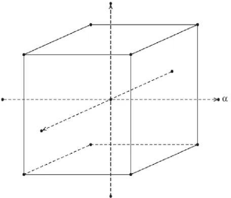
analyzed by statistical methods, resulting in valid and objective conclusions [7]. There are various experimental designs used by researchers to plan their experiments they include; factorial design, Central Composite Design (CCD), Response Surface Methodology (RSM) and Taguchi methods. They are now widely used in place of one-factor-at-a-time experimental approach which is time consuming and exorbitant in cost. In other words, Rotatable Central Composite Design commonly referred to as (RCCD) is used in designing experiments by selecting optimally cutting parameter values. RCCD is shown diagrammatically in Fig. 2 as equation (1) satisfies the rotatability criteria, where α is the points at the centre and 𝑛 is number of factors.

Fig. 2: Central Composite Design with rotatability

α = 2𝑛/4 (1)

In RCCD, the required number of experimental points or runs 𝑁 is given by

𝑁 = 2𝑛 + 2𝑛 + 𝑛_𝑟 (2)

Where 𝑛_𝑟 is the replicate centre point or repeated average level.

Kurt, Suruculer and Ali [6] experimentally investigated cutting forces which occurred during metal cutting, analyzed the effects of cutting forces on the cutting tool by means of ANSYS software and mathematically modelled the primary cutting force and the stresses using the acquired findings. Another approach which involves the use of dynamometer to measure experimental cutting forces and analytically fitting the force model has been applied by Feng and Menq [8]. They designed a 2-D cutting force model, without considering cutting force along the cutter axis. Yang and Tarng [9] applied the Taguchi method to find the optimal cutting parameters for

turning operations. An orthogonal array, the signal-to-noise (S/N) ratio and the Analysis of Variance (ANOVA) were employed to investigate the cutting characteristics of S45C steel bars using tungsten carbide cutting tools. Chen [10] investigated the cutting forces and surface finish when machining medium hardened steel using CBN tools, while Darwish [11] studied the impact of the tool material and the cutting parameters on surface roughness of nickel super alloy. Also, Huang and Liang [12] modelled the cutting forces under hard turning conditions considering tool wear effect. Finally, Wassila [13] optimized the cutting parameters to minimize the production time in high speed turning.

The aforementioned investigators have actually performed studies on modelling of cutting forces using optimization techniques, effort will be made in this study to simplify and adopt these techniques in order to solve a local problem by modelling axial cutting forces generated during a typical orthogonal turning of mild steel shaft using cutting tools commonly used in local lathe shops; carbide and HSS tools. RCCD will be used for the plan of experiments and axial cutting forces will be measured using a spring-based dynamometer. A non-linear empirical cutting force model shown in equation (3) formulated by Tlusty [5] will be used in estimating these cutting force coefficients.

𝐹_𝑥 = 𝐾𝑤𝑓_𝑥𝛼 (3)

Equation (3) is transformed into a first-order linear model by taking the natural logarithm of both sides of it as follows

𝑙𝑜𝑔 𝐹_𝑥 = 𝑙𝑜𝑔 𝐾 + 𝑙𝑜𝑔 𝑤 + 𝛼 𝑙𝑜𝑔𝑓_𝑥 (4)

Equation (1.4) can as well be expressed as follows

𝑌 = 𝐾₀ + 𝐾₁𝑋₁ + 𝐾₂𝑋₂ ± 𝜀 (5)

In equation (5) 𝑌 is the logarithmic value of the response variable or the cutting force component, 𝐾_𝑖(𝑖 = 0, 1, 2 … ) is the cutting force coefficients, 𝑋₁ and 𝑋₂ are the logarithmic values of the predictor variables; depth of cut 𝑤 and the feed rate 𝑓_𝑥 respectively and 𝜀 is the error term. The solution of equation (5) is obtained by setting up the sum of squares of the residuals and differentiating with respect to each of the unknown coefficients. The solution is expressed as follows

𝐾_𝑖 = [𝑋′∙ 𝑋]−1∙ 𝑋′∙ 𝑌 (6)

(3)

𝑤 = 𝑀𝜔𝑛2𝑤𝐷

𝐾𝛼( 𝑓𝑥)𝛼–1 (7)

Ω = 30𝜔𝑛Ω𝐷

𝜋 (8)

Where 𝜔_𝑛 is the cutting tool natural frequency and 𝑀 is its dynamic mass. 𝑤_𝐷 and Ω_𝐷 are both dimensionless form of depth of cut and spindle speed respectively.

II.EXPERIMENTALDETAILS

A.Materials

The materials used for the experiments as shown in Fig. 3 are carbide tool brazed on a flexural steel shank of dimension 100𝑚𝑚× 12 𝑚𝑚× 12𝑚𝑚 and High Speed Steel cutting tool of the same cross-section. The choice of these two cutting tools lies on their application in local lathe shops. Mild steel rod sample of 35𝑚𝑚diameter and 280𝑚𝑚 long was used as the workpiece.

Fig. 3: Cutting tools and workpiece used during turning test [16]

B.Method

In this study, turning process was studied using RCCD to select cutting parameters at 𝑛 = 2 factors. Equation (1) gives α =√2 = 1.414 for 𝑛 = 2. Using equation (2) 𝑁= 12 is calculated as the required number of experimental points or runs for the RCCD as shown in TABLE I, since there are eight factorial experiments with added 6 star points and centre point (average level) repeated 6 times to calculate pure error [7, 17]. TABLE I shows the experimental plan based on RCCD used in selecting parameter values.

TABLEI

PHYSICAL AND CODED VALUES OF CUTTING PARAMETERS IN RCCDFOR CARBIDE AND HSS TOOL-WORKPIECE COMBINATION

Symbol Factors Lowest Low Centre High Highest

Coding for

RCCD

-1.414 - 1 0 1 1.414

A Feed (𝑚𝑚/𝑟𝑒𝑣)

= 𝑓

0.076 0.22 0.36 0.50 0.64

B Depth of cut

(𝑚𝑚) = 𝑤

0.10 0.45 0.80 1.15 1.50

C.Setup and Experimentation

(4)

Fig. 4: Dry orthogonal turning process of mild steel sample and cutting force measurement using dynamometer [16]

TABLEII

ROTATABLE CENTRAL COMPOSITE DESIGN OF EXPERIMENT AT

𝑁=12 FOR CARBIDE TOOL-MILD STEEL PAIR

A B 𝑭_𝒙_(N)

- 1 - 1 140.50

1 - 1 139.90

- 1 1 235.50

1 1 245.10

0 0 154.50

0 0 146.60

0 0 255.50

0 0 250.20

- 1.414 0 226.00

1.414 0 226.00

0 - 1.414 226.00

0 1.414 226.00

TABLEIII

ROTATABLE CENTRAL COMPOSITE DESIGN OF EXPERIMENT AT

𝑁=12 FOR HSS TOOL-MILD STEEL PAIR

A B 𝑭_𝒙 (N)

- 1 - 1 124.50

1 - 1 121.00

- 1 1 216.50

1 1 220.00

0 0 130.50

0 0 132.00

0 0 138.20

0 0 239.50

- 1.414 0 208.00

1.414 0 208.00

0 - 1.414 208.00

0 1.414 208.00

III. RESULTSANDDISCUSSION

A.Bi-variate Least-Squares Analysis

The statistical analysis software Microsoft Excel 2007 was used in solving the bi-variate equation (6) in a least-squares sense in order to determine the cutting force coefficients for the carbide and HSS tool-workpiece combination respectively as follows;

TABLE IV

LOGARITHMIC TRANSFORMATION OF VARIABLES FOR CARBIDE TOOL-MILD STEEL PAIR

𝒍𝒐𝒈 A 𝒍𝒐𝒈 B 𝒍𝒐𝒈 𝑭_𝒙

−0.65758 −0.34679 2.188928

−0.30103 −0.34679 2.389343

−0.65758 0.060698 2.166134

−0.30103 0.060698 2.407391

−0.4437 −0.09691 2.354108

− 0.4437 −0.09691 2.354108

−1.11919 − 0.09691 1.860937

−0.19382 −0.09691 2.355068

(5)

−0.4437 0.176091 2.362671

TABLE V

LOGARITHMIC TRANSFORMATION OF VARIABLES FOR HSS TOOL-MILD STEEL PAIR

𝒍𝒐𝒈 A 𝒍𝒐𝒈 B 𝒍𝒐𝒈 𝑭_𝒙

−0.65758 −0.34679 2.095169

−0.30103 −0.34679 2.335458

−0.65758 0.060698 2.115611

−0.30103 0.060698 2.379306

−0.4437 −0.09691 2.318063

− 0.4437 −0.09691 2.318063

−1.11919 − 0.09691 1.662758

−0.19382 −0.09691 2.345374

−0.4437 −1.0000 2.258877

−0.4437 0.176091 2.34557

The first-order linear model for the carbide-HSS tool-workpiece combinations are shown in equation (9) and (10) respectively as

𝑌_{𝑐𝑎𝑟𝑏𝑖𝑑𝑒} = 2.63 𝑋₀ + 0.06 𝑋₁+ 0.66 𝑋₂ ± 0.03 (9)

𝑌ℎ𝑠𝑠 = 2.61 𝑋0 + 0.007 𝑋1+ 0.76 𝑋2 ± 0.075 (10)

It is observed from equation (9) and (10) that their coefficients of determination 𝑅2 are given as 95% and 82% as well as their errors 𝜀 to be 3.0% and 7.5% respectively. Also, by taking their inverse logarithms their cutting force coefficients are summarized in TABLE VI.

TABLE VI

CUTTING FORCE COEFFICIENT AND FEED EXPONENT FROM THE FIRST-ORDER EMPIRICAL MODEL FOR CARBIDE AND HSS

TOOL-WORKPIECE COMBINATIONS

Cutting Tool Cutting Force Coefficient

𝑲𝒊 (𝑵-𝒎−

𝟏𝟑 𝟖)

Feed Exponent 𝜶_𝒊

Carbide 4.27 ×108 0.66

HSS 4.07 ×108 0.76

B.Stability Prediction of Turning Process

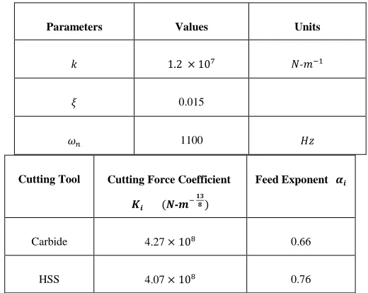
The parameters that will be assumed to approximate those used in this study were adopted from Ozlu and Budak [14]. The choice of these parameters is based on the fact that modal testing kits needed to generate experimentally modal parameters are exorbitant and are quite sophisticated for local use. Careful observation of the cutting tools used in this study is comparable with that found in TABLE VII gotten experimentally and used by Ozlu and Budak [14] in plotting stability diagram of low speed full immersion turning of medium carbon steel (AISI 1040) workpiece. TABLE VII shows the modal parameters used in this study for stability prediction during turning operation.

TABLE VII

EXPERIMENTAL MODAL PARAMETERS ADOPTED FROM OZLU AND BUDAK [14] FOR CHATTER PREDICTION

Where 𝑘 is the tool stiffness 𝜉 = 𝑐

2√𝑀𝑘 is the damping factor of cutting tool which typically have low values 𝜉 between 0.005−0.02 and 𝜔_𝑛 the natural frequency of cutting tool. Using the relation 2𝜋𝜔_𝑛(𝐻𝑧) = 𝜔_𝑛(𝑟𝑎𝑑𝑠−1) the tool natural frequency is given as 𝜔_𝑛= 6912.4 𝑟𝑎𝑑𝑠−1 and

dynamic mass 𝑀 = 𝑘 _𝜔 𝑛2

� = 0.25 𝑘𝑔.

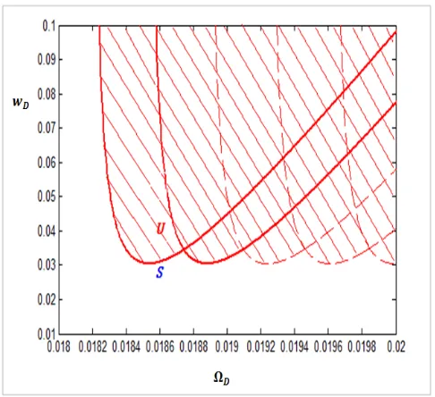
A stability lobe diagram for a turning process can be plotted on the Ω_𝐷− 𝑤_𝐷 plane using DDE23 subroutine in MATLAB. Assuming the chatter frequency 𝜔 rose from 0 to 10000 𝑟𝑎𝑑𝑠−1 slightly higher than the tool natural frequency a stability diagram is plotted and displayed as figure 5. Each stability lobe is identified by its number 𝑗 and for each lobe Ω_𝐷=1⁄ 𝑗 . In Fig. 5, 𝑗= 1⁄Ω_𝐷 = 1⁄0.0186 ≈55

Parameters Values Units

𝑘 1.2 × 107 _𝑁_-_𝑚−1

𝜉 0.015

(6)

lobes for the tool. Also Ω_𝐷 = 0.0186 corresponds to the highest operating spindle speed Ω= 1230 𝑟𝑝𝑚 of the lathe system used in the study. Also, portion shaded red and the point with red U-mark on the stability diagram indicates region of instability that are prone to chatter and should be avoided at all cost by the machinist, while the region below that is not shaded is stable. During a typical turning operation, the choice of the co-ordinate (0.0186, 0.0300) as shown on the stability diagram with a blue S-mark is a maximum stable turning operation for the lathe system used in the study.

When performing turning operation at the highest feed using carbide and HSS tool-mild steel pairs, their stable operational depth of cuts and spindle speeds are given by equation (7) and (8) respectively. TABLE VIII shows maximum operational depth of cut at highest spindle speed and feed gotten for both tool-workpiece combinations in this study.

It is observed from TABLE VIII that a maximum stable turning operation for carbide tool is at 0.1 𝑚𝑚 and that of HSS tool at 0.2 𝑚𝑚. This shows that the Material Removal Rate (MRR) or shearing effect of carbide tools is less than that of HSS tools and that the latter is dynamically stable when turning under the same machining condition.

Fig. 5: Stability diagram of turning operation for 𝑗= 1 to 55

TABLE VIII

MAXIMUM OPERATIONAL DEPTH OF CUT AT HIGHEST SPINDLE SPEED AND FEED GOTTEN FOR BOTH TOOL-WORKPIECE

COMBINATIONS

Cutting Tool

Cutting Force Coefficient

(𝑁-𝑚−138)

Feed

Exponent

Feed rate

(𝑚𝑚/𝑟𝑒𝑣)

Operational

Depth of Cut

(𝑚𝑚)

Carbide 4.27 ×108 0.66 0.64 0.1

HSS 4.07 ×108 0.76 0.64 0.2

IV. CONCLUSION

This paper presents the findings of an experimental study based on RCCD into determining cutting force coefficients from axial cutting forces and using them to predict dynamic stability when turning mild steel shafts with carbide and HSS tools respectively. Modeling of axial cutting force was done using a non-linear empirical force law, which was later made linear by logarithmic transformation. The results gotten after bi-variate least-squares regression revealed that the cutting force coefficients of carbide tools are slightly higher than that of HSS tools. The results also indicate that the (MRR) or shearing effect of carbide tools are less than that of HSS tools and that the latter is dynamically stable when turning under the same machining condition, so effort should be made through material and cutting tool modification to render these coefficients low in order to minimize tool chatter and to achieve higher productivity during turning operations.

ACKNOWLEDGMENT

This research is supported by Electronic Development Institute (www.eldiawka.org). They gave access to their Dean Smith & Grace Lathe machine.

REFERENCES

[1] Youssef, & El-Hofy, H., (2008) Machining technology: Machine tools and operations, CRC Press Taylor & Francis Group, New York. [2] Dunwoody, K., (2010) Automated identification of cutting force coefficients and tool dynamics on CNC machines. Master’s thesis, University of British Columbia Vancouver.

[3] Dimitri, G., Fromentin, G., Poulachon, G., & Bissey, B. S., (2013) From large-scale to micro machining: A review of force prediction models. Journal of Manufacturing Processes, Vol. 15, p.389–401. [4] Kienzle, O., & Victor, H., (1957) “Spezifische Shnittkraefte bei der Metall-bearbeitung’’, Werkstattstehnik und Maschinenbau, Bd. 47, H.5.

[5] Tlusty, J., (2000) Manufacturing process and equipment, Prentice Hall, Englewood Cliffs, NJ.

[6] Kurt, A., Sürücüler, S., & Ali, K., (2010) Developing a mathematical model for the cutting forces prediction depending on the cutting parameters. Gazi University, Technical Education Faculty, Ankara. Gazi University, Institute of Science, Ankara. Technology, 13(1), 23-30.

[7] Montgomery, D., (2003) Design and analysis of experiments, 5th Edition, John Wiley & Sons, Inc., New York.

[8] Feng, H. S., Menq, C. H., (1994) The prediction of cutting forces in ball-end milling process: Model formulation and model building process. International Journal of Machine Tools & Manufacture, 34: 697–710.

(7)

[10] Chen, W., (2000) Cutting forces and surface finish when machining medium hardness steel using CBN tools. Int. J. Mach. Tools Manuf. 40, 455–466.

[11] Darwish, S. M., (2000) The impact of tool material and the cutting parameters on surface roughness of supermet 718 Nickel super alloy. J. Mater. Process. Technol. 97, 10–18.

[12] Huang, Y., & Liang, S. Y., (2005) Modelling of cutting forces under hard turning conditions considering tool wear effect. ASME J. Manuf. Sci. Eng. 127, 262–270.

[13] Wassila, B., (2005) Cutting parameter optimization to minimize production time in high speed turning. Journal of Materials Processing Technology (161); 388–395.

[14] Ozlu, E., & Budak, E., (2006) Analytical modelling of chatter stability in turning and boring operations—Part I: Model development, ASME J. Manuf. Sci. Eng. Vol. 129, no 4, pp. 726–732. [15] Stepan, G. R., Szalai, R., & Insperger, T., (2003) Nonlinear dynamics of high-speed milling subjected to regenerative effect: To appear in the book, Nonlinear dynamics of production systems, edited by Gunther Radons, Wiley-VCH, New York.

[16] Ezeanyagu, P. I., (2015) Cutting force coefficients estimation and tool dynamics of turning process, “Unpublished” Master of Engineering thesis, Nnamdi Azikiwe University Awka.