A Generalized Neural Network Approach to Mobile Robot Navigation and Obstacle Avoidance

(1)

Electronic Theses and Dissertations Theses, Dissertations, and Major Papers

2012

A Generalized Neural Network Approach to Mobile Robot

Navigation and Obstacle Avoidance

Seyyed Hamid Dezfoulian University of Windsor

Follow this and additional works at: https://scholar.uwindsor.ca/etd

Recommended Citation Recommended Citation

Dezfoulian, Seyyed Hamid, "A Generalized Neural Network Approach to Mobile Robot Navigation and Obstacle Avoidance" (2012). Electronic Theses and Dissertations. 102.

https://scholar.uwindsor.ca/etd/102

(2)

A Generalized Neural Network Approach to

Mobile Robot Navigation and Obstacle Avoidance

by

Hamid Dezfoulian

A Thesis

Submitted to the Faculty of Graduate Studies through Computer Science

in Partial Fulfillment of the Requirements for the Degree of Master of Science at the

University of Windsor

Windsor, Ontario, Canada

2011

(3)

A Generalized Neural Network Approach to Mobile Robot Navigation and Obstacle

Avoidance

by

Hamid Dezfoulian

APPROVED BY:

______________________________________________ Dr. Jonathan Wu

Department of Electrical and Computer Engineering

______________________________________________ Dr. Alioune Ngom

School of Computer Science

______________________________________________ Dr. Imran Ahmad, Co-Advisor

______________________________________________ Dr. Dan Wu, Advisor

______________________________________________ Dr. Yung H. Tsin, Chair of Defense

(4)

DECLARATION OF ORIGINALITY

I hereby certify that I am the sole author of this thesis and that no part of this

thesis has been published or submitted for publication.

I certify that, to the best of my knowledge, my thesis does not infringe upon

anyone’s copyright nor violate any proprietary rights and that any ideas, techniques,

quotations, or any other material from the work of other people included in my thesis,

published or otherwise, are fully acknowledged in accordance with the standard

referencing practices. Furthermore, to the extent that I have included copyrighted

material that surpasses the bounds of fair dealing within the meaning of the Canada

Copyright Act, I certify that I have obtained a written permission from the copyright

owner(s) to include such material(s) in my thesis and have included copies of such

copyright clearances to my appendix.

I declare that this is a true copy of my thesis, including any final revisions, as

approved by my thesis committee and the Graduate Studies office, and that this thesis has

(5)

ABSTRACT

In this thesis, we tackle the problem of extending neural network navigation

algorithms for various types of mobile robots and 2-dimensional range sensors. We

propose a general method to interpret the data from various types of 2-dimensional range

sensors and a neural network algorithm to perform the navigation task. Our approach can

yield a global navigation algorithm which can be applied to various types of range

sensors and mobile robot platforms. Moreover, this method allows the neural networks to

be trained using only one type of 2-dimensional range sensor, which contributes

positively to reducing the time required for training the networks. Experimental results

carried out in simulation environments demonstrate the effectiveness of our approach in

mobile robot navigation for different kinds of robots and sensors. Therefore, the

successful implementation of our method provides a solution to apply mobile robot

(6)

DEDICATION

This thesis is dedicated to my parents who taught me the value of education and

for their endless love, support and encouragement. I am deeply indebted to them for their

(7)

ACKNOWLEDGEMENTS

I would like to express my sincere thanks to my supervisor, Dr. Dan Wu for

giving me an opportunity to pursue a Master's program and for his support, guidance and

patience throughout this project whilst allowing me the room to work in my own way. I

would also like to express my thanks to Dr. Imran Ahmad for accepting to be my

co-supervisor and for his guidance and motivation throughout this research project and

lavishly, providing the primers.

Gratitude is also expressed to my committee: Dr. Alioune Ngom for his

invaluable support and guidance during my first steps into the field of machine learning

and pattern recognition and Dr. Jonathan Wu for his detailed and constructive comments.

Finally, I am eternally grateful to my father for his support, guidance and help in

all the time of research and writing of this thesis. With his help in countless ways it was

(8)

LIST OF TABLES

TABLE 1:COMMON ACTIVATION FUNCTIONS IN USE WITH NEURAL NETWORKS.[17,22] .... 10

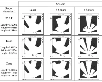
TABLE 2:EXAMPLES OF SENSOR READINGS OF DIFFERENT SENSORS FROM THREE DIFFERENT

MOBILE ROBOTS. ... 75

TABLE 3:EXAMPLES OF TRAINING PATTERNS FOR TRAINING A) THE ACTION-SVM, AND B)

THE DIRECTION-SVM... 79

TABLE 4:COMPARISON OF THREE FEATURE EXTRACTION METHODS FOR TRAINING ANN-A,

(11)

LIST OF FIGURES

FIGURE 1:A SIMPLE (ARTIFICIAL) NEURON [17] ... 8

FIGURE 2:A VERY SIMPLE NEURAL NETWORK [17] ... 9

FIGURE 3: A)A SINGLE-LAYER NEURAL NET. B)A MULTI-LAYER NEURAL NET.[17] ... 12

FIGURE 4:BACKPROPAGATION NEURAL NETWORK WITH ONE HIDDEN LAYER.[17] ... 16

FIGURE 5:CHOOSING THE HYPERPLANE THAT MAXIMIZES THE MARGIN [55] ... 26

FIGURE 6:RELATIONSHIPS BETWEEN MOBILE ROBOT RESEARCH AREAS.[63] ... 28

FIGURE 7: A)MODIFIED PCANEURAL NETWORK TOPOLOGY. B)WORKSPACE SEGMENTS. [18] ... 34

FIGURE 8:TOPOLOGY OF MULTI-LAYER PERCEPTRON.[18] ... 35

FIGURE 9:FOUR-LAYER NEURAL NETWORK FOR ROBOT NAVIGATION.[20,21] ... 36

FIGURE 10:MONODA MODULAR SYSTEM.[8] ... 36

FIGURE 11: A)LOCALISATION OF NOMAD 200™ SENSORS. B)NOMAD MOBILE ROBOT. C) MODULAR ARCHITECTURE.[8] ... 37

FIGURE 12:FLOWCHART OF PROPOSED METHOD ... 39

FIGURE 13:EXAMPLE OF SCENARIOS OF WALL-FOLLOWING, OBJECT-AVOIDANCE AND TARGET-SEEKING TASKS ... 41

FIGURE 14:PATHS SHOWING TWO DIFFERENT DIRECTIONS CHOSEN WHEN ENCOUNTERING A WALL. ... 41

FIGURE 15:PATH OF A WALL-FOLLOWING TASK PERFORMED BY A MOBILE ROBOT ONLY IN KEEP-LEFT DIRECTION. ... 42

(12)

FIGURE 17: A)EXAMPLE OF VISUALIZING THE DATA FROM A LASER RANGE FINDER INTO A

BINARY IMAGE. B)EXAMPLE OF VISUALIZING THE DATA FROM 8 SONAR SENSORS INTO

A BINARY IMAGE. ... 45

FIGURE 18:PROPOSED NEURAL NETWORK ARCHITECTURES FOR A)ANN-A, B)ANN-B AND ANN-C ... 47

FIGURE 19:CONCEPT OF THE MOTION CONTROLLER WITH RESPECT TO STEERING ANGLES. 51 FIGURE 20:A MOBILE ROBOT WITH 8 SONAR SENSORS... 56

FIGURE 21:A MOBILE ROBOT WITH A RANGESCANNER (LASER RANGE FINDER).[91] ... 57

FIGURE 22: A)MECHANICAL P2AT. B)SIMULATED P2AT.[89] ... 58

FIGURE 23: A)MECHANICAL P2DX. B)SIMULATED P2DX.[89] ... 58

FIGURE 24: A)MECHANICAL ATRVJR. B)SIMULATED ATRVJR.[89] ... 58

FIGURE 25: A)MECHANICAL ZERG. B)SIMULATED ZERG.[89] ... 59

FIGURE 26: A)MECHANICAL TRANTULA. B)SIMULATED TRANTULA.[89] ... 59

FIGURE 27: A)MECHANICAL TALON. B)SIMULATED TALON.[89] ... 60

FIGURE 28:PROGRAMMING STRUCTURE SCHEMA ... 61

FIGURE 29: A)ENVIRONMENT SAMPLE B)RANGESCANNER VISUALIZATION C)SONAR SENSOR VISUALIZATION ... 63

FIGURE 30: A)ENVIRONMENT SAMPLE B)RANGESCANNER VISUALIZATION C)SONAR SENSOR VISUALIZATION ... 64

FIGURE 31:FLOWCHART OF ALGORITHM IMPLEMENTED IN MATLAB. ... 65

FIGURE 32:3-LAYER ARTIFICIAL NEURAL NETWORK (ANN-A) ... 67

(13)

FIGURE 35:MOBILE ROBOT'S PATH A) WITHOUT A WALL-FOLLOWING ALGORITHM B) WITH A

WALL-FOLLOWING ALGORITHM, WHEN ENCOUNTERING A U-SHAPED OBSTACLE. ... 70

FIGURE 36:TWO OBSTACLE-AVOIDANCE EXAMPLES IN MOBILE ROBOT MOTION CONTROL. A)90° ROTATION TO THE RIGHT B)45° ROTATION TO THE RIGHT. ... 71

FIGURE 37:DIFFERENT SENSOR DISTRIBUTIONS. A) LASER RANGE SCANNER. B)8 SONAR SENSORS. C)5 SONAR SENSORS. ... 74

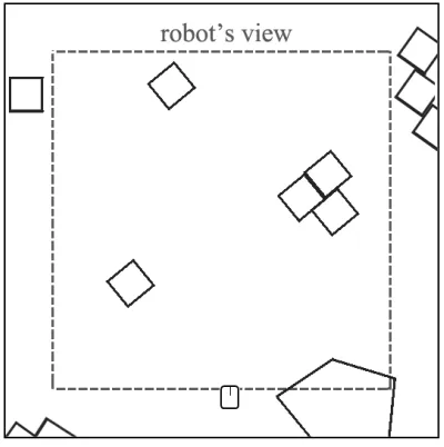
FIGURE 38:AN EXAMPLE OF ROBOTS VIEW IN AN ENVIRONMENT. ... 74

FIGURE 39:A2D TOP VIEW OF OUR TRAINING ENVIRONMENT FOR OBJECT-AVOIDANCE. ... 76

FIGURE 40:A3D VIEW OF OUR TRAINING ENVIRONMENT FOR OBJECT AVOIDANCE. ... 76

FIGURE 41:A2D TOP VIEW OF OUR TRAINING ENVIRONMENT FOR WALL-FOLLOWING. ... 78

FIGURE 42:A3D VIEW OF OUR TRAINING ENVIRONMENT FOR WALL-FOLLOWING ... 78

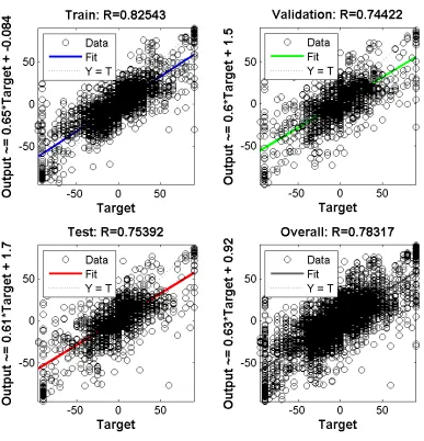
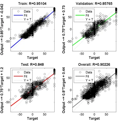
FIGURE 43:REGRESSION PLOTS FOR TRAINING ANN-A WITH 3000 TRAINING SAMPLES AND 3000 SAMPLES FOR TESTING AND VALIDATION. ... 82

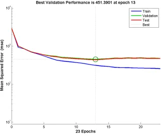
FIGURE 44:PERFORMANCE PLOT FOR TRAINING ANN-A ... 83

FIGURE 45:REGRESSION PLOTS FOR TRAINING ANN-B WITH 1500 TRAINING SAMPLES AND 1500 SAMPLES FOR TESTING AND VALIDATION. ... 84

FIGURE 46:REGRESSION PLOTS FOR TRAINING ANN-C WITH 1500 TRAINING SAMPLES AND 1500 SAMPLES FOR TESTING AND VALIDATION. ... 85

FIGURE 47:PERFORMANCE PLOT FOR TRAINING ANN-B ... 86

FIGURE 48:PERFORMANCE PLOT FOR TRAINING ANN-C ... 86

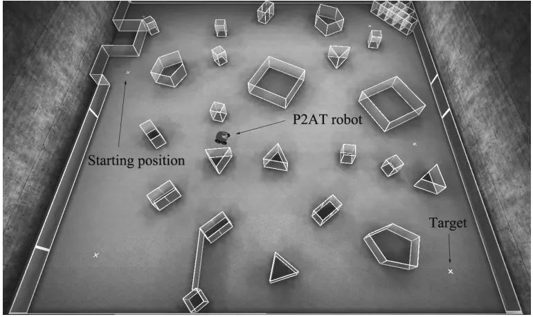
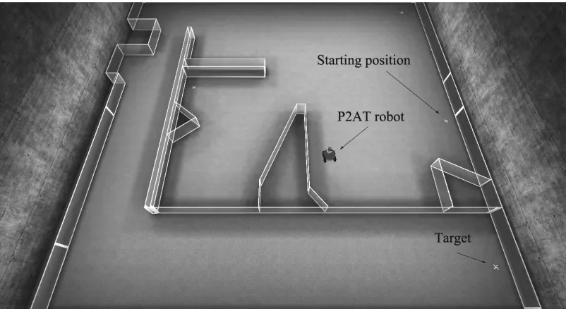
FIGURE 49:FOUR ENVIRONMENTS USED FOR TESTING OUR ALGORITHM ... 87

(14)

FIGURE 52:SIMULATION RESULTS FOR P2AT USING THREE DIFFERENT SENSORS IN

ENVIRONMENT 1... 90

FIGURE 53:SIMULATION RESULTS FOR TALON USING THREE DIFFERENT SENSORS IN

ENVIRONMENT 1... 90

FIGURE 54:SIMULATION RESULTS FOR ZERG USING THREE DIFFERENT SENSORS IN

ENVIRONMENT 1... 91

FIGURE 55:SIMULATION RESULTS FOR P2AT,TALON AND ZERG USING LASER RANGE

SCANNER IN ENVIRONMENT 1. ... 91

FIGURE 56:SIMULATION RESULTS FOR P2AT,TALON AND ZERG USING 8-SONAR SENSORS

IN ENVIRONMENT 1. ... 92

FIGURE 58:SIMULATION RESULT FROM [19] IN ENVIRONMENT #2 ... 94

FIGURE 59:SIMULATED ENVIRONMENT #2 IN UNREAL TOURNAMENT ENGINE ... 94

ENVIRONMENT #2... 95

FIGURE 63:SIMULATION RESULTS FOR P2AT,TALON AND ZERG USING LASER SCANNER IN

(15)

IN ENVIRONMENT #2 ... 97

FIGURE 66:SIMULATION RESULT FROM [19] IN ENVIRONMENT #2 ... 99

FIGURE 67:SIMULATED ENVIRONMENT #3 IN UNREAL TOURNAMENT ENGINE ... 99

FIGURE 71:SIMULATION RESULTS FOR P2AT,TALON AND ZERG USING LASER SCANNER IN

FIGURE 74:SIMULATION OF ENVIRONMENT #4 IN UNREAL TOURNAMENT ENGINE ... 104

(16)

FIGURE 78:SIMULATION RESULTS FOR P2AT,TALON AND ZERG USING LASER RANGE

SCANNER IN ENVIRONMENT #4 ... 106

(17)

Chapter 1 Introduction

1.1 Motivation

Navigation is one of the most important problems in designing and developing

intelligent mobile robots. Staying operational, i.e. avoiding dangerous situations such as

collisions and staying within safe operating conditions (temperature, radiation, exposure

to weather, etc.) comes first. But if any tasks are to be performed that relate to specific

places in the robot environment, navigation is a must.

Robot navigation is defined by the ability of a mobile robot to determine its own

position in its frame of reference and then to plan a path towards some goal location [1].

In order to navigate in an environment, the mobile robot requires representation, i.e. a

map of the environment, and the ability to interpret that representation. Therefore

navigation can be defined as the combination of the three fundamental abilities [1]:

 _{Self-Localisation}  Path Planning

 Map-Building and Map-Interpretation

In this context, map represents any mapping of the environment onto an internal

representation. Moreover, Robot localization indicates the ability of the robot to establish

its own position and orientation within the frame of reference.

Path planning is effectively an extension of localization, in that it requires the

determination of the robot's current position and a position of a goal location, both within

(18)

reactive. The inputs to the mobile robot navigator are the target position and the sensor

system data. If there are no obstacles between the robot and its target, the navigation path

is just a straight line between them. If an obstacle is detected, some avoidance strategy is

required. Potential function based methods [2,3], neural networks [4-9], and fuzzy logic

based controllers [10-13], trained with a heuristic database of rules, are among the

possibilities.

Finally, Map-Building can be in the form of a metric map or any notation

describing locations in the frame of reference.

In the past few years, neural networks including feedforward neural network,

self-organizing neural network, principal component analysis (PCA), dynamic neural

network, support vector machines (SVM), neuro-fuzzy approach, etc., [14,15] have been

extensively used in mobile robot navigation field [16]. This is due to their assets such as

nonlinear mapping, ability to learn from examples, good generalization performance,

massively parallel processing, and ability to approximate any function given adequate

number of neurons.

Sensors are necessary for a robot to know where it is or how it got there, or to be

able to reason about where it has to go. The sensors may be roughly divided into two

classes: internal state sensors, such as accelerometers, gyroscopes, and external state

sensors, such as laser sensors, infrared sensors, sonar, and visual sensors. The data from

internal state sensors are used for estimating the position of the robot in a 2-dimensional

space. The data from external state sensors provide information that can be used to

(19)

object. Due to the inevitable sensor noise, in most cases, the sensor readings are

inaccurate and unreliable. Therefore, it is essential for the navigation algorithm to process

the sensor data with noises. Since neural networks have many processing nodes, each

with primarily local connections, they may provide some degree of robustness or fault

tolerance for interpretation of the sensor data. [16]

However, most of the current research addresses one particular type of sensor or

robot platform. The main issue with neural network approaches is the training of the

network. Collecting sufficient, yet valuable, samples from the environment to train the

network can sometimes be frustrating and very time consuming [17]. In addition, apart

from the effort that has to be put to collect valuable samples, the training time of a

network can be significantly high [17]. In any neural network navigation algorithm, if the

robot platform or the type or number of the sensors are changed or altered, the network

architecture requires some modifications to accommodate with the new amount of sensor

data. Moreover, new training samples need to be gathered as the previous samples will

not be as much useful for the new robot platform. In other words, when a network

structure is designed for a specific type of sensor, it cannot be used for other types or

different numbers of sensors. By changing the structure of the network, therefore, new

training samples are required and the network needs to be trained from the beginning.

This presents challenge and opportunity to develop a general method to interpret sensor

data from different types of sensors that can yield a global navigation algorithm which

(20)

1.2 Contributions

This thesis is concerned with the problem of generalizing the interpretation of

sensory data and mobile robot navigation. The contributions of this thesis are as follows:

The primary contribution of this thesis is to develop a general method for

interpretation of different types of sensors, such as laser and ultrasonic sensors. Our

approach extends the work done by Janglová [18] for determining the free-spaces by

applying PCA Neural Network (PCNN). We study the problem of how current neural

network navigation approaches are limited to one type of sensor and the kinematic

constraints of a mobile robot. Our approach however is extendable to various

2-dimensional sensors and mobile robots. On the other hand, this approach allows the

neural networks to be trained using only one type of sensor which contributes positively

to reducing the training time. Experimental results, carried out in simulated

environments, demonstrate that our approach can be positively affective in mobile robot

navigation for different kinds of robots and sensors, when compared to previous works.

Therefore, the successful implementation of our method provides a solution to apply

navigation algorithms to various robot platforms.

The second important contribution of this thesis is to implement an algorithm to

perform the navigation task using our interpretation of sensory data. Our approach is

inspired by the works done by Parhi and Singh [19-21] for neural network robot

navigation. Parhi and Singh introduced a real-time obstacle avoidance approach, solving

each of the target-seeking, obstacle-avoidance, and wall-following tasks with separate

(21)

instead of using two separate networks, we introduce a structure which uses only one

network for this purpose. Yet, the wall-following task will require a more complex

structure to accommodate with both directions of rotation. Therefore, our proposed

method for mobile robot navigation can yield significant navigation results for various

sensors and robots – at less training time and lower sensor costs.

The third contribution of this thesis is that we develop a software application to

carry out the proposed approach. The experimental results obtained through this

application indicate feasibility of our approach in simulation robots.

1.3 Guide to the Thesis

This thesis is organized as follows.

Chapter 2: Background Knowledge. This chapter provides an introduction to

the subjects that the proposed method builds upon. After explaining the concept of

artificial neural networks and backpropagation algorithm, some methods of feature

extraction and classification will be given. The Principal Component Neural Network

(PCNN) method and Support Vector Machine (SVM) algorithms are specifically

emphasized, since they constitute the core of the proposed approach. The attention then

moves to the discussion of mobile robot navigation and its current applications.

Chapter 3: Design and Methodology. The proposed interpretation of sensory

data and mobile robot navigation method based on neural networks is presented in detail

in this chapter. First the definition of the problem is described, followed by detailed

presentation of the proposed approach.

(22)

results section, experiments carried out for training and experiments done for testing on

simulation robots are described. Finally, these experimental results are compared with

experimental results from previous methods and the evaluations are obtained.

Chapter 5: Conclusion and Future Work. This final chapter brings conclusion

(23)

Chapter 2 Background Knowledge

This chapter provides the background knowledge on which the proposed method

is based on. After explaining Artificial Neural Networks (ANN), feature extraction

methodology, specifically Principal Component Analysis (PCA), is described.

Consequently, a method of classification, Support Vector Machines (SVM), is illustrated.

Finally, current robot navigation and obstacle avoidance algorithms are reviewed with a

view to the applications of artificial neural networks in robot navigation and obstacle

avoidance.

2.1 Artificial Neural Networks

Artificial neural networks are information-processing systems which have certain

performance characteristics in common with biological neural networks [22]. Artificial

neural networks have been evolved as generalizations of mathematical models of human

cognition or neural biology, based on the following four assumptions [17]:

1. "Information processing occurs at many simple elements called neurons."

2. "Signals are passed between neurons over connection links."

3. "Each connection link has an associated weight, which, in a typical neural net,

multiplies the signal transmitted."

4. "Each neuron applies an activation function (usually nonlinear) to its net input (sum

of weighted input signals) to determine its output signal."

(24)

determining the weights on the connections (called its training, or learning, algorithm),

and finally, its activation function.

Neural networks are structured from a large number of simple processing

components called neurons, units, cells, or nodes. Each neuron is connected to other

neurons through directed communication links, each with a weight associated to it (as

shown in Figure 1). The weights correspond to information being processed by the

network to solve a problem. Neural networks can be applied to a wide selection of

problems, such as storing and recalling data or patterns, grouping similar patterns,

performing general mappings from input patterns to output patterns, classifying patterns,

or finding solutions to constrained optimization problems.[17,22]

Figure 1: A simple (artificial) neuron [17]

The internal state of a neuron is known as its activation or activity level, which is

a function of the inputs it has received. Typically, activation is sent as a signal from one

neuron to several other neurons. However, only one signal can be sent from each neuron

at the same time, although that signal can be broadcast to several other neurons. For

example, consider neuron 𝑌, shown in Figure 1, that receives inputs from neurons 𝑋₁, 𝑋₂,

and 𝑋3. The activations (output signals) of these neurons are 𝑥1, 𝑥2, and 𝑥3, respectively.

(25)

and 𝑤3, respectively. The net input, 𝑦_𝑖𝑛, to neuron 𝑌 is the sum of the weighted signals

from neurons 𝑋1, 𝑋2, and 𝑋3, that is:

𝑦_𝑖𝑛= 𝑤1𝑥1+𝑤2𝑥2+𝑤3𝑥3

The activation 𝑦 of neuron 𝑌 is given by some function of its net input,

𝑦= 𝑓(𝑦_𝑖𝑛), for example, the logistic sigmoid function (an S-shaped curve)

𝑓(𝑥) =_{1 + e}1 _−x

or any of a number of other activation functions (see Table 1 for a number of common

activation functions in use with neural networks).

Further, suppose that neuron 𝑌 is connected to neurons 𝑍1, and 𝑍2, with weights

𝑣1, and 𝑣2, respectively, as depicted in Figure 2. neuron 𝑌 sends its signal 𝑦 to each of

these units. However, generally, the values received by neurons 𝑍₁, and 𝑍₂ will be

different. Since each signal is scaled by the appropriate weight, 𝑣₁ or 𝑣2. As shown in

this simple example, in a typical network, the activations 𝑧₁ and 𝑧₂ of neurons 𝑍₁, and 𝑍₂

would depend on inputs from several neurons and not just one. [17]

Figure 2: A very simple neural network [17]

Even though the neural network in Figure 2 is very simple, the presence of an

(26)

solved by a network with only input and output units. However, the difficulty to train

(i.e., find optimal values for the weights) a net with hidden units is more than a network

with no hidden units.

Table 1: Common activation functions in use with neural networks. [17,22]

Function Definition Range

a) Identity 𝑥 (−∞, +∞)

b) _SigmoidBinary 1

1 +𝑒−𝑥 (0, +1)

c) _SigmoidBipolar 1− 𝑒−𝑥

1 +𝑒−𝑥 (−1, +1)

d) Hyperbolic 𝑒𝑥− 𝑒−𝑥

𝑒𝑥₊_𝑒−𝑥 (−1, +1)

e) - Exponential 𝑒−𝑥 _{(0, +}_∞₎

f) Softmax 𝑒𝑥

∑ 𝑒_𝑖 𝑥𝑖 (0, +1)

g) Unit sum _{∑ 𝑥}𝑥

𝑖

𝑖 (0, +1)

h) Square root _√𝑥 (0, +∞)

i) Sine sin(𝑥) [0, +1]

j) Ramp �−𝑥 1 −1 <𝑥𝑥 ≤ −< +11

+1 𝑥 ≥+1� [−1, +1]

(27)

2.1.1 Typical Architectures

Often, it is more convenient to visualize neurons arranged in layers. Normally,

neurons that are in the same layer behave in the same manner. The key factors in

determining the behaviour of a neuron are activation function and the pattern of weighted

connections. Within each layer, neurons typically have the same activation function and

the same pattern of connections with other neurons.

The arrangement of neurons into layers and the connection patterns within and

between layers is known as the network architecture [17]. Many neural networks have an

input layer in which the activation of each unit is equal to an external input signal. The

network presented in Figure 2 consists of three input units, two output units, and one

hidden unit (a unit that is neither an input unit nor an output unit).

Neural networks are typically classified into two categories; single layer and

multilayer. Since no computation is performed by the input units, they are not counted as

a layer when determining the number of layers. Similarly, the number of layers in the

network can be defined as the number of layers of weighted interconnected links between

the layers of neurons. This point of view is motivated by the fact that the weights in a

network have extremely important information [17]. The network depicted in Figure 2

has two layers of weights.

Illustrated in Figure 3 are examples of single-layer and multilayer feedforward

networks—networks in which the signals flow in a forward direction from the input units

(28)

Figure 3: a) A single-layer neural net. b) A multi-layer neural net.[17]

For pattern classification, each output unit corresponds to a particular category to

which an input vector may or may not belong. Note that in a single-layer net, the weights

of output units will not be influenced by the weights of other output units. For pattern

association, the same architecture can be used; however the overall pattern of output

signals gives the response pattern associated with the input signal that caused it to be

produced. These two examples illustrate that depending on the interpretation of the

response of the network, the same type of network can be used for different problems.

Alternatively, for more complicated mapping problems a multilayer network maybe

required. The problems that require multilayer networks may still represent classification

or association of patterns. Although the type of problem affects the choice of architecture,

but it does not exclusively determine it.

(29)

weights between two adjacent layers of units (input, hidden, or output). Multilayer

networks can solve more complex problems than single-layer networks can, but training

may be more complicated. Nevertheless, in some cases, training may be more successful,

since it is possible to solve problems that single-layer networks cannot be trained to

perform correctly at all. [22]

In addition to the architecture, the method of setting the values of the weights

(training) is an important distinguishing attribute of various neural networks. Typically,

neural networks are distinguished by two types of training—supervised and

unsupervised; furthermore, there are networks whose weights are fixed without an

iterative training process. [17,22]

Various tasks that neural nets can be trained to carry out fall into areas such as

mapping, clustering, and constrained optimization. Pattern classification and pattern

association may be considered special forms of the more general problem of mapping

input vectors or patterns to the specified output vectors or patterns. [22]

Possibly, in the most standard neural network setting, training is achieved by

introducing a series of training vectors, or patterns, each with an associated target output

vector. Then based on a learning algorithm the weights are adjusted. This process is

called supervised training [17]. Some of the simplest neural networks are designed to

perform pattern classification that is to classify an input vector as either it belongs to or

does not belong to a given category. In this type of neural network, the output is a

bivalent element, say, either 1 (if the input vector belongs to the category) or −1 (if it

(30)

networ k, such as that trained by back propagation may be better as will be described in

the next section.

Pattern association is another special form of a mapping problem, where in which

the desired output is not just a "yes" or "no", but rather a pattern. Associative memory

[17] is a neural network which is trained to associate a group of input vectors with a

corresponding group of output vectors. If the desired output vector is the same as the

input vector, the network is called an auto-associative memory [17]; moreover, if the

output target vector is different from the input vector, the network is a hetero-associative

memory [17]. Following training, an associative memory can recall a stored pattern when

it is provided an input vector that is adequately similar to a vector it has learned.

Multilayer neural networks can be trained to perform a nonlinear mapping from an

𝑛-dimensional space of input vectors (𝑛-tuples) to an 𝑚-𝑛-dimensional output space—i.e., the

output vectors are 𝑚-tuples.[22]

On the other hand, in unsupervised training, self-organizing neural networks [22]

group similar input vectors together without using training data to specify what a typical

member of each group looks like or to which group each vector belongs. A series of input

vectors is provided, but no target vectors are specified. The network adjusts the weights

so that the most similar input vectors are assigned to the same output (or cluster) unit.

Hence, the neural network will produce an exemplar (representative) vector for each

cluster formed.

2.1.2 Backpropagation Neural Net

(31)

extensive spreading of an effective general method for training a multilayer neural

network [23-26] played a major role in the comeback of neural networks as a tool for

solving a wide variety of problems.

The backpropagation network is a multilayer feedforward network trained by

backpropagation which can be used to solve problems in many areas. Applications using

such networks can be found in almost any area that uses neural networks to solve

problems involving mapping a given set of inputs to a particular set of target outputs, i.e.

networks that use supervised training. The aim in most neural networks is to train the

network to attain a balance between the capability to respond correctly to the input

patterns that are used for training (memorization) and the capability to give reasonable

(good) responses to input that is similar, but not identical, to that used in training

(generalization). [17]

Training a network with backpropagation comprises of three stages: the

feedforward of the input training pattern, the calculation and backpropagation of the

associated error, and the adjustment of the weights [17]. Subsequent to training,

application of the network involves only the computations of the feedforward phase. A

trained network can produce its output very fast even if training is slow. While a

single-layer network is very limited in the mappings it can learn, a multisingle-layer network (with one

or more hidden layers) can learn any continuous mapping to any desired accuracy. For

some applications more than one hidden layer may be beneficial, however one hidden

layer is usually adequate [22].

(32)

have biases. The bias on a standard output unit 𝑌𝑘 is denoted by 𝑊0𝑘; the bias on a typical

hidden unit 𝑍_𝑦 is denoted 𝑉_0𝑗. These bias terms function like weights on connections

from units whose output is always 1 [17]. Only the direction of information flow for the

feedforward phase is shown. During the backpropagation phase of learning, signals are

sent in the reverse direction. The algorithm in APPENDIX A is presented for one hidden

layer, which is adequate for a large number of applications.

Figure 4: Backpropagation neural network with one hidden layer.[17]

An activation function for a backpropagation network should have several

important characteristics: It should be continuous, differentiable, and monotonically

non-decreasing. In addition, for computational efficiency, it is beneficial that its derivative be

easy to compute. For the most frequently used activation functions, some of which

(33)

maximum and minimum values asymptotically [17]. The binary sigmoid function,

illustrated in Table 1 (b) is one of the most typical activation functions; another common

activation function is the bipolar sigmoid function (Table 1 (c)). Note that the bipolar

sigmoid function is closely related to the hyperbolic function (Table 1(d)).

The mathematical basis for the backpropagation algorithm is the optimization

technique called the gradient descent. The gradient of a function (in the case of

backpropagation, the function is the error and the variables are the weights of the

network) gives the direction in which the function increases more rapidly; the negative

value of the gradient gives the direction in which the function decreases most rapidly

[27]. The derivation clarifies the reason why the weight updates described in APPENDIX

A should be done after all of the 𝛿𝑘 and 𝛿𝑗 expressions have been calculated, rather than

during backpropagation.

2.2 Feature Extraction

In pattern recognition and image processing, feature extraction is a particular type

of dimensionality reduction.

When the data is too large to be processed by an algorithm and it is also suspected

to be extremely redundant, the input data can be transformed into a reduced

representation set of features (also called features vector) by feature extraction methods.

If the extracted features are carefully chosen, it is expected that the features set will

extract the important information from the data in order to perform the desired task with

this reduced representation instead of the entire data.

(34)

complex data rises from the number of variables involved. Analysis with a large number

of variables typically requires large amount of memory and computation power or a

classification algorithm which usually over fits the training samples and generalizes

poorly to new patterns. Feature extraction is used as a general term for methods for

constructing combinations of variables to get around these problems while still describing

the data with sufficient accuracy.

Best results are attained when an expert constructs a set of application-dependent

features. Nonetheless, if no such expert knowledge is available general dimensionality

reduction techniques may be of assistance [28-34].

2.2.1 Principal Component Analysis (PCA)

The most commonly used approach for extracting features from a set of observed

variables is perhaps Principal Components Analysis (PCA). PCA is a mathematical

procedure where an orthogonal transformation is used to convert a set of observations of

possibly correlated variables into a set of values of uncorrelated variables known as

principal components [34,35]. The number of extracted principal components is less than

or equal to the number of original variables. The transformation of the data is defined in

such a way that the first principal component has the highest variance possible i.e.,

constitutes as much of the variability in the data as possible. Moreover, each subsequent

component in turn has as high a variance as possible under the constraint that it be

orthogonal to (uncorrelated with) the preceding components. If the data set is jointly

normally distributed, principal components are guaranteed to be independent. However,

(35)

PCA was invented in 1901 by Karl Pearson [37]. PCA has a wide range of

applications some of which include data compression, image processing, visualization,

exploratory data analysis, pattern recognition, and time series prediction. A complete

discussion of PCA can be found in [22,38]. Usually after mean centering the data for

each attribute, PCA can be achieved by eigenvalue decomposition of a data covariance

matrix or singular value decomposition of a data matrix. Typically, the results of a PCA

are discussed in terms of component scores (the transformed variable values

corresponding to a particular case in the data) and loadings (the weight by which each

standardized original variable should be multiplied to get the component score). [36,39]

The popularity of PCA appears from three important assets. First, it is the optimal

(in terms of mean squared error) linear scheme for compressing a set of high dimensional

vectors into a set of lower dimensional vectors and then reconstructing the original set.

Second, the model parameters can be computed directly from the data - for example by

diagonalizing the sample covariance matrix. Third, given the model parameters,

compression and decompression are simple operations to perform where they require

only matrix multiplication. [36,39,40]

Perhaps, PCA's operation is better thought as exposing the internal structure of the

data in a way which best explains the variance in the data. If a multivariate dataset is

visualised as a set of coordinates in a high-dimensional data space (1 axis per variable),

PCA can supply the user with a lower-dimensional picture [36,39]. This is achieved by

using only the first few principal components so that the dimensionality of the

(36)

PCA is mathematically defined as an orthogonal linear transformation [40] which

transforms the data to a new coordinate system such that the largest variance by any

projection of the data comes to lie on the first coordinate (known as the first principal

component), the second largest variance on the second coordinate, and so on.

To calculate the principal components we define a data matrix, 𝑋𝑇_{, with zero}

empirical mean (the sample mean of the distribution is subtracted from the data set),

where each of the 𝑛 rows stands for a different repetition of the experiment, and each of

the 𝑚 columns provides a particular kind of datum e.g., the results from a particular

probe. The singular value decomposition of 𝑋 is 𝑋=𝑊Σ𝑉𝑇_{, where the 𝑚}_×_{𝑚 matrix 𝑊}

is the matrix of eigenvectors of 𝑋𝑇_{𝑋, the matrix Σ is an 𝑚}_×_{𝑛 rectangular diagonal}

matrix with nonnegative real numbers on the diagonal, and the 𝑛×𝑛 matrix 𝑉 is the

matrix of eigenvectors of 𝑋𝑇_{𝑋. The PCA transformation that preserves dimensionality}

i.e., gives the same number of principal components as original variables is then given

by:

𝑌𝑇 ₌_𝑋𝑇_𝑊

=𝑉Σ𝑇

In the usual case when 𝑀 <𝑛 −1, 𝑉 is not uniquely defined. However, 𝑌 will

usually still be uniquely defined. Since 𝑊 (by definition of the SVD of a real matrix [41])

is an orthogonal matrix where each row of 𝑌𝑇_{is simply a rotation of the corresponding}

row of 𝑋𝑇_{. The first column of}_𝑌𝑇_{is created from the}_scores_{of the instances with respect}

to the principal component; the next column has the scores with respect to the second

(37)

If a reduced-dimensionality representation is required, we can project 𝑋 down into

the reduced space defined by only the first 𝐿 singular vectors, 𝑊𝐿:

𝑌= 𝑊𝐿𝑇𝑋=Σ𝐿𝑉𝐿𝑇

The matrix 𝑊 of singular vectors of 𝑋 is equivalently the matrix 𝑊 of

eigenvectors of the matrix of observed covariance 𝐶 =𝑋𝑋𝑇_,

𝑋𝑋𝑇 ₌ _𝑊ΣΣ𝑇_𝑊𝑇

The first principal component corresponds to a line that passes through the

multidimensional mean and minimizes the sum of squares of the distances of the points

from the line provided a set of points in Euclidean space. The second principal

component relates to the same concept after all correlation with the first principal

component has been subtracted out from the points. The singular values (in Σ) are the

square roots of the eigenvalues of the matrix 𝑋𝑋𝑇_{. Each eigenvalue is proportional to the}

portion of the variance that is correlated with each eigenvector. More correctly they are

proportional to the portion of the sum of the squared distances of the points from their

multidimensional mean. The sum of all the eigenvalues is equal to the sum of the squared

distances of the points from their multidimensional mean. Basically, PCA rotates the set

of points around their mean in order to align with the principal components. This moves

as much of the variance as possible, by using an orthogonal transformation, into the first

few dimensions. Therefore, the values in the remaining dimensions tend to be small and

may be ignored with minimal loss of information. PCA is often used in this manner for

dimensionality reduction. Therefore, it has the distinction of being the optimal orthogonal

(38)

2.2.2 Principal Component Neural Networks (PCNN)

Since the original work of Oja and his research group, principal component

analysis by neural networks and its extensions have become an important research field

(a partial list of references is given by [41-47]) both for the interesting implications on

unsupervised learning theory and applications to neural information processing [48].

The algorithms considered in this section are based on Oja's principal component

neuron described by 𝑧(𝑡) =𝒒𝑇₍_𝑡₎_𝒙₍_𝑡₎_{, where 𝒙}₍_𝑡₎_{∈ ℛ}𝑝_{represents the stationary}

multivariate random process whose first principal component is looked for, 𝒒(𝑡)∈ ℛ𝑝_is

the neuron's weight vector, and 𝑧(𝑡) ∈ ℛ is the neuron's output signal. Oja's learning rule

[47] is:

𝒒(𝑡+ 1) = 𝜂𝒙(𝑡)𝑧(𝑡) +𝒒(𝑡)[1− 𝜂𝑧2₍_𝑡_)]

where 𝜂 is a small learning rate and 𝑡 indicates discrete time. This expression clearly

reveals the presence of the Hebbian term +𝒙(𝑡)𝑧(𝑡) [49] and of a stabilizing term, thus it

is also referred to as stabilized Hebbian learning equation.

The Generalized Hebbian Algorithm by Sanger [49] is one among the best known

learning algorithms that allow a linear neural network to extract a selected number of

principal components from a stationary or quasi-stationary multivariate random process.

It applies to a single-layered feedforward neural network described by 𝒛(𝑡) =𝑸𝑇₍_𝑡₎_𝒙₍_𝑡₎_,

where 𝒙(𝑡)∈ ℛ𝑝_{, 𝒛}₍_𝑡₎ _{∈ ℛ}𝑚_{, thus 𝑸}₍_𝑡₎ _{∈ ℛ}𝑝×𝑚_{. The GHA rule writes:}

𝑸(𝑡+ 1) = 𝜇𝒙(𝑡)𝒛𝑇₍_𝑡_{) +}_𝑸₍_𝑡₎₍_𝑰

𝑚− 𝜇𝐿𝑇[𝒛(𝑡)𝒛𝑇(𝑡)])

where 𝑚 is a small positive learning rate, the operator 𝐿𝑇[⋅] returns the lower-triangular

(39)

rule is an extension of Oja's rule, where the neurons are forced to encode different

features by means of intrinsic Gram-Schmidt orthogonalization [50].

Kung and Diamantaras developed a learning rule (Laterally-Connected Network

and Apex Rule) for Rubner-Tavan's principal component neural network [51] described

by the following input-output relationships:

𝒛(𝑡) =𝑸𝑇₍_𝑡₎_𝒙₍_𝑡_),

𝒚(𝑡) =𝒛(𝑡) +𝑯𝑇₍_𝑡₎_𝒚₍_𝑡_).

where the input vector 𝒙(𝑡) ∈ ℛ𝑝_{, the output vector}_𝒚₍_𝑡₎_{∈ ℛ}𝑚_(with_{𝑚 ≤ 𝑝}_{, arbitrarily}

fixed), the direct-connection weight-matrix 𝑸(𝑡) ∈ ℛ𝑝×𝑚_{and the lateral-connection}

strictly upper-triangular weight-matrix 𝑯(𝑡)∈ ℛ𝑚×𝑚_{are evaluated at the same time. The}

Kung-Diamantaras' APEX learning rule for the weight-matrix 𝑸 and the inhibitory

weight-matrix 𝑯 recasts from [48] in matrix notation:

𝑸(𝑡+ 1) = 𝜇𝑿(𝑡)𝒀�(𝑡) +𝑸(𝑡)�𝑰𝑚− 𝜇𝒀�2(𝑡)�

𝑯(𝑡+ 1) = −𝜇𝑆𝑈𝑇�𝒀(𝑡)𝒀�(𝑡)�+𝑯(𝑡)[𝑰𝑚− 𝜇𝒀�2(𝑡)]

where 𝑚 is a small positive learning rate, matrices 𝑿 ∈ ℛ𝑝×𝑚_,_{𝒀 ∈ ℛ}𝑚×𝑚_{, and 𝒀� ∈}

ℛ𝑚×𝑚_{are defined by:}

𝑿 ≜[��𝐱𝐱 ⋅⋅⋅ 𝐱]

𝑚

,𝒀 ≜[_{��}𝐲𝐲 ⋅⋅⋅ 𝐲]

𝑚

,𝒀� ≜diag(y1, y2, … , ym)

and operator 𝑆𝑈𝑇 [⋅] returns the strictly upper-triangular part of the matrix contained

within. Kung-Diamantaras' rule has been heuristically derived by applying Oja's rule to

direct-connection weight-vectors, and its anti-Hebbian version to lateral-connection

(40)

2.2.3 Non-negative Matrix Factorization (NMF)

Unsupervised learning algorithms such as principal component analysis can be

known as factorizing a data matrix subject to different constraints. Based on the

employed constraints, the resulting features can be shown to have very different

representational properties. [34,52,53].

NMF is described as to find non-negative matrix factors 𝑊 and 𝐻, given a

non-negative matrix 𝑉, such that:

𝑉 ≈ 𝑊𝐻

NMF can be used for the statistical analysis of multivariate data in the following

approach: Given a series of multivariate 𝑛-dimensional data vectors, the vectors are

placed in the columns of an 𝑛×𝑚 matrix 𝑉 where 𝑚 is the number of samples in the

dataset. Matrix 𝑉 is then approximately factorized into an 𝑛×𝑟 matrix 𝑊 and an 𝑟×𝑚

matrix 𝐻. Typically, 𝑟 is chosen to be smaller than 𝑛 or 𝑚, so that 𝑊 and 𝐻are smaller

than the original matrix 𝑉. This results in a compressed form of the original data matrix

[53].

The significance of approximating 𝑉 ≈ 𝑊𝐻 is that it can be rewritten column by

column as 𝑣 ≈ 𝑊ℎ, where 𝑣 and ℎ are the corresponding columns of 𝑉 and 𝐻. More

formally, each data vector 𝑣 is approximated by a linear combination of the columns of

𝑊, which is weighted by the components of ℎ. Hence, 𝑊 can be considered as to contain

a basis that is optimized for the linear approximation of the data in 𝑉. Since relatively

small amount of basis vectors are used to represent many data vectors, high quality

(41)

2.3 Support Vector Machine (SVM) Classification

Classification, in machine learning and pattern recognition, refers to an

algorithmic procedure for assigning a set of input data to one of a given number of

categories [15]. An example would be predicting the species of a flower given petal and

sepal measurements [54]. An algorithm that implements classification, particularly in a

solid implementation, is called a classifier [15]. The term "classifier" sometimes also

refers to the mathematical function, implemented by a classification algorithm, which

maps input data to a category.

Typically, classification refers to a supervised procedure, i.e. a procedure that

learns to classify new samples based on learning from a training set of instances that have

been properly labelled with the correct classes by hand. The corresponding unsupervised

method is known as clustering. This procedure involves grouping data into different

classes based on some measure of inherent similarity [14] (e.g. the distance between

instances, considered as vectors in a multi-dimensional vector space).

The support vector machine (SVM) [55-58] is a training algorithm for learning

classification and regression rules from data. For instance SVM can be used to learn

polynomial, radial basis function (RBF) and multi-layer perceptron (MLP) classifiers

[58]. In the 1960s, Vapnik first suggested SVMs for classification. Recently, support

vector machines have become an area of extreme research mainly because of the

developments in the techniques and theory joined with extensions to regression and

density estimation.

(42)

intermediate step [58]. SVMs are based on the structural risk minimisation principle

which is closely related to regularisation theory. This principle features capacity control

to prevent over-fitting and therefore is a partial solution to the bias-variance trade-off

dilemma [59].

In the implementation of SVM, there are two main components; techniques of

mathematical programming and kernel functions. The parameters are found by solving a

quadratic programming problem with linear equality and inequality constraints; rather

than by solving a non-convex, unconstrained optimisation problem [56]. SVM is able to

search a wide variety of hypothesis due to the flexibility of the kernel functions. The

geometrical interpretation of support vector classification (SVC) is that the algorithm

searches for the optimal separating surface (hyperplane) that is, in a sense, equidistant

from the two classes [55] (see Figure 5). Statistical properties of this optimal separating

(43)

Without requiring a separate validation set during training, the SVM parameters

can be optimized using generalisation theory. As SVM is based on solid statistical and

mathematical foundations concerning generalisation and optimisation theory, hence, it

has been proven to outperform existing techniques on a wide variety of real world

problems [56]. SVMs and related methods are also being increasingly applied to real

world data mining. An up-to-date list of such applications can be found at [60].

2.4 Mobile Robot Navigation and Obstacle Avoidance

In the past few years, mobile robots have been widely used in various fields, such

as space exploration, industrial and military industries, under water survey, and service

and medical applications, hence attracting the attention from researchers. Mobile robots

require the capabilities of autonomy and intelligence, therefore, researchers are forced to

deal with important issues such as uncertainty (in both sensing and action), reliability,

and real-time response [61]. As a result, one of the major challenges in robotics is

designing algorithms to allow the robots to function autonomously in unstructured,

dynamic, partially observable, and uncertain environments [62]. Figure 6 shows the

position of motion control (for obstacle avoidance) and exploration (navigation)

(44)

Figure 6: Relationships between mobile robot research areas. [63]

The problem of mobile robot navigation, includes three fundamental matters; map

building, localization and path planning. This problem refers to planning a path to a

specified target, executing this plan based on sensor readings, and is the key to the robot

performing some particular tasks. Artificial Neural networks are increasingly being used

in various fields of machine learning, including pattern recognition, speech production

and recognition, signal processing, medicine, and business. In the recent years, artificial

neural networks, including feedforward neural network, self-organizing neural network,

principal component analysis (PCA), dynamic neural network, support vector machines

(SVM), neuro-fuzzy approach, etc., have been extensively employed in the field of

mobile robot navigation because of their properties such as nonlinear mapping, ability to

learn from examples, good generalization performance, massively parallel processing,

and ability to approximate an arbitrary function given sufficient number of neurons

(45)

2.4.1 Neural Networks for Interpretation of the Sensor Data

For a mobile robot to identify where it is or how it got there, or to be able to

reason about where it has gone, sensors are necessary. For measuring the distance that

wheels have traveled along the ground and for measuring inertial changes and external

structure in the environment, the sensors can be flexible and mobile. The sensors can be

generally divided into two categories: internal state sensors, and external state sensors.

The internal state sensors such as accelerometers and gyroscopes, provide the internal

information about the robot’s movements. The external state sensors, such as laser,

infrared sensors, sonar, and visual sensors, provide the external information about the

environment. The data from internal state sensors can be used to estimate the position of

the robot in a 2-dimensional space; however, cumulative error is inevitable. The data

from external state sensors can be applied for recognizing a place or a situation, or be

used to construct a map of the environment. Laser, infrared, and sonar sensors can obtain

distant and directional information about an object. Visual sensors can also provide rich

information of the environment, but can be very expensive to process. In most cases,

because of the available noises, the sensor readings are imprecise and unreliable. Thus, it

is inevitable for the mobile robot navigation algorithm to process the sensor data with

noises. Given that neural networks have many processing units, each with primarily local

connections, they may provide some degree of robustness or fault tolerance for

interpretation of the sensor data [16].

Feedforward multi-layer perception neural network, trained by the

(46)

"translate" the readings of sonar sensors into occupancy values of each grid cell for

building metric maps. Meng and Kak proposed a NEURO-NAV system for mobile robot

navigation [65]. In the NEURO-NAV, in order to drive the robot to move in the middle

of the hallway, a feedforward neural network, which is driven by the cells of the Hough

transformation of the corridor guidelines in the camera image, is used to obtain the

approximate relative angles between the heading direction of the robot and the orientation

of the hallway [65]. self-organizing Kohonen neural networks are well known for their

capability to carry out classification, recognition, data compression and association in an

unsupervised manner [66]. In [67], self-organizing Kohonen neural networks are applied

to recognize landmarks using the measurements from laser sensors in order to provide

coordinates of the landmarks for triangulation.

As mentioned before, PCA is a statistical technique, which has been applied to

machine learning fields such as data compression and pattern recognition, and is known

as one of the effective techniques to extract the principal features from high-dimension

data and reduce the dimension of the data [40]. In [68], Vlassis et al. presented an

approach for mobile robot localization where PCA was used to reduce the dimensions of

sonar sensor data. Crowley et al. proposed an approach to estimate the position of a

mobile robot based on the PCA of laser ranger sensor data [69]. In [70,71], PCA has been

used to extract features of images for mobile robot localization. PCA Neural Network

(PCNN) was applied for navigation to determine the "free space" in front of a mobile

robot using ultrasound range finder data in order to construct a collision-free path for the

(47)

2.4.2 Neural Networks for Obstacle Avoidance

There are always static, as well as non-static obstacles in the environment. Hence,

robots need to autonomously navigate themselves in environments by avoiding obstacles.

The neural networks, which have been designed for obstacle avoidance by mobile robots,

should take the sensor data from the environment as their inputs, and output the direction

for the robot to proceed. In [72], Fujii et al. presented a multilayered neural network

model through reinforcement learning for collision avoidance of a mobile robot. Silva et

al. proposed the MONODA (MOdular Network for Obstacle Detection and Avoidance)

architecture for obstacle avoidance and detection of a mobile robot in unknown

environments [8]. This model consists of four three-layered feedforward neural network

modules where each module detects the probability of obstacles in one direction of the

robot. In [73], Ishii et al. developed an obstacle avoidance method based on

self-organizing Kohonen neural networks for underwater vehicles. Gaudiano and Chang

proposed an approach for obstacle avoidance by employing a neural network model of

classical and operant conditioning based on Grossberg’s conditioning circuit [7,74]. Parhi

and Singh introduced a real-time obstacle avoidance approach to solve each of the

target-seeking, obstacle-avoidance, and wall-following tasks using separate neural networks

[19-21]. In their approach, based on certain criteria one of the networks is selected at

each time step to control the mobile robot allowing it to move safely in a crowded

real-world and unknown environment and to reach a specified target while avoiding static as

(48)

2.4.3 Neural Networks for Path Planning

The path planning problem may consist of two sub-problems; path generation and

path tracking. This problem refers to determining a path between an initial pose of the

mobile robot and a final pose such that the robot does not collide with any objects in the

environment and that the planned motion is consistent with the kinematic constraints of

the vehicle. The existing path planning methods include A* algorithm [75], potential

fields [2], and methods using intelligent control technique such as neural networks and

neuro-fuzzy. Methods using intelligent control do not plan global paths for mobile robots

and can be employed in unknown environments. The input pattern of the neural networks

employed for path planning of mobile robots should consider the following data: robot’s

actual position and velocities; robot’s previous positions and velocities; target position

and sensor data, and then output commands to drive the robot to follow a path towards

the target by avoiding obstacles according to these data [16].

Kozakiewicz and Ejiri have used a human expert to train a feedforward neural

network that reads inputs from a camera and outputs the appropriate commands to the

actuators [76]. In [77], Sfeir et al. presented a path generation technique for mobile robot

using memory neuron network proposed by Sastry et al. [78]. The memory neuron

network is a feedforward neural network that uses memory neurons. A memory neuron is

a combination of a classic perception and unit delays, which gives the network memory

abilities. If a mobile robot is totally insensitive to context, it will often get trapped in

oscillations in front of wide objects. Pal and Kar employed a notion of memory into the

(49)

learning. Fierro and Lewis proposed a control structure which integrates a kinematic

controller with a feedforward neural network computed-torque controller for

non-holonomic mobile robots, where the neural network weights are adjusted on-line, with no

"off-line learning phase" needed [80-82]. Yang and Meng studied a biologically inspired

neural network approach for motion planning of mobile robots [83-85]. This model is

inspired by Hodgkin and Huxley’s membrane model [86] for a biological neural system

and Grossberg’s shutting model [87]. The proposed model by Yang and Meng plans

motions for mobile robots without any prior knowledge of the environment, without

explicitly searching over the free workspace or the collision path, and without any

(50)

Chapter 3 Design and Methodology

As reviewed in chapter2, Janglová [18] introduced an intelligent controller for

solving the motion-planning problem in mobile robots using two neural networks. The

first neural network is a modified principal component analysis network (Figure 7(a))

used to extract the features (𝑉𝑖 segments) of the workspace determining the free space

using the data from ultrasound range finders (𝑑_𝑖) as shown in Figure 7(b). These

segments (𝑉_𝑖) are used as inputs to the second neural network along with direction of the

goal (𝑆_𝑖). The second network is a multilayer perceptron (Figure 8), which successfully

finds a safe direction (𝑂𝑖), from the segments extracted from the first network, for the

robot's next step to navigate towards the target in a collision-free environment while

avoiding obstacles.

(51)

Figure 8: Topology of Multi-Layer Perceptron. [18]

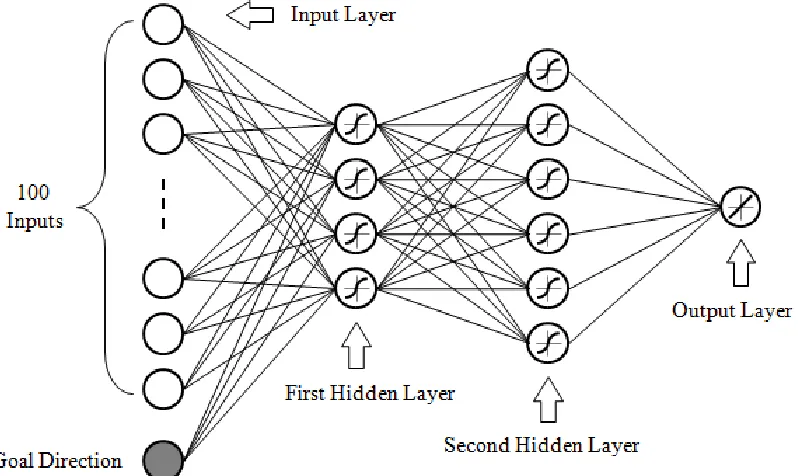
Parhi and Singh [20,21] proposed a real-time obstacle avoidance method to solve

the main problems of navigation using three neural networks. This approach was later

improved by them to optimize the path of the mobile robot [19]. In their approach, three

identical four-layer feedforward neural networks have been used (see Figure 9). Each

network is trained separately with different training samples so that each network can

solve one of the problems of navigation; target-seeking, object-avoidance, or

wall-following. The inputs to their proposed neural controller consist of the signals from the

sensors (in this case, the distance from the left, right and front obstacle with respect to the

robot's position) and the direction of the target (goal). The output of the networks is the

steering angle which provides real-time collision-free motion planning for mobile robots

in a real world dynamic environment. The neural networks are trained by presenting them

(52)

Figure 9: Four-layer neural network for robot navigation. [20,21]

In [8] Silva et al. presented the MONODA (modular network for obstacle

detection and avoidance) architecture for obstacle detection and avoidance for controlling

the NOMAD autonomous mobile robot in an unknown environment (see Figure 10). As

depicted in Figure 11(c), this model consists of four three-layered feedforward neural

network modules (each detects the probability of obstacle in one direction of the robot).

The convention in neural networks is to use architectures as small as possible to obtain

(53)

Figure 11: a) Localisation of Nomad 200™ sensors. b) Nomad mobile robot.

c) Modular architecture. [8]

With modular networks generalisation is improved, because each one of the

network modules is easier to train well. Due to the modular architecture, usually, the

number of weights is less than in a fully connected MLP. Therefore, the overall training

time of the networks is also significantly reduced.

3.1 Problem Statement

Although all the described methods have been successful to some extent in their

specific applications, however, most of the current approaches address one particular type

of sensor or robot platform. The main problem with neural network approaches is the

A Generalized Neural Network Approach to Mobile Robot Navigation and Obstacle Avoidance

A Generalized Neural Network Approach to Mobile Robot

A Generalized Neural Network Approach to Mobile Robot

Navigation and Obstacle Avoidance

Navigation and Obstacle Avoidance

A Generalized Neural Network Approach to

Mobile Robot Navigation and Obstacle Avoidance

DECLARATION OF ORIGINALITY

ABSTRACT

DEDICATION

ACKNOWLEDGEMENTS

TABLE OF CONTENTS

LIST OF TABLES

LIST OF FIGURES

Chapter 1

Introduction

1.1

Motivation

1.2

Contributions

1.3

Guide to the Thesis

Chapter 2

Background Knowledge

2.1

Artificial Neural Networks

2.1.1 Typical Architectures

2.1.2 Backpropagation Neural Net

2.2

Feature Extraction

2.2.1 Principal Component Analysis (PCA)

2.2.2 Principal Component Neural Networks (PCNN)

2.2.3 Non-negative Matrix Factorization (NMF)

2.3

Support Vector Machine (SVM) Classification

2.4

Mobile Robot Navigation and Obstacle Avoidance

2.4.1 Neural Networks for Interpretation of the Sensor Data

2.4.2 Neural Networks for Obstacle Avoidance

2.4.3 Neural Networks for Path Planning

Chapter 3

Design and Methodology

3.1

Problem Statement