Relationships Between Prior Experiences, Current Teaching Contexts, and Novice Teachers' Use of Concrete Representation for Mathematics Instruction

(1)

University of South Carolina

Scholar Commons

Theses and Dissertations

2014

High Throughput Multi-Solution Genetic

Algorithm (HTMGA) for Identification of

Alternate Solutions in a Structural Model Updating

Context

Muslum Kilinc

University of South Carolina - Columbia

Follow this and additional works at:https://scholarcommons.sc.edu/etd

Part of theCivil and Environmental Engineering Commons

This Open Access Dissertation is brought to you by Scholar Commons. It has been accepted for inclusion in Theses and Dissertations by an authorized administrator of Scholar Commons. For more information, please [email protected].

Recommended Citation

(2)

High Throughput Multi-Solution Genetic Algorithm (HTMGA) For Identification Of Alternate Solutions In A Structural Model

Updating Context

by

Muslum Kilinc

Bachelor of Civil Engineering Dokuz Eylul University 2001

Master of Engineering University of South Carolina 2010

Submitted in Partial Fulfillment of the Requirements for the Degree of Doctor of Philosophy in

Civil Engineering

College of Engineering and Computing University of South Carolina

2014 Accepted by:

Juan M. Caicedo, Major Professor Robert L. Mullen, Committee Member

Joseph Flora, Committee Member Jianjun Hu, Committee Member

(3)

c

(4)

Dedication

(5)

Acknowledgments

(6)

Abstract

(7)

List of Tables

Table 2.1 Possible Multiple Solutions for Run 1 (fα = 1.5 and ∆ = 5%) . . . 15

Table 2.2 Possible Multiple Solutions for Run 2 (fα = 1.5 and ∆ = 15%) . . 17

Table 2.3 Possible Multiple Solutions for Run 3 (fα = 1.5 and ∆ = 25%) . . 18

Table 3.1 Parameters for HTMGA to Run One Variable Function . . . 27

Table 3.2 Parameters for HTMGA to Run Two Variable Function . . . 29

Table 3.3 Number of Multiple Solutions are found with 50,100, 200, 500, 1000, 2000, 5000 Population Size . . . 31

Table 3.4 Number of True and False Solutions are found with Distance<0.015 32 Table 3.5 Number of Multiple Solutions are found with Mutation Percent-ages of 5, 10, 20, 25, 30, 50 . . . 34

Table 3.6 Number of True and False Solutions are found with Distance<0.015 34 Table 4.1 Section and Material Properties for Illustrative Test Structure . . . 38

Table 4.2 Experimental (References) Natural Frequencies . . . 39

Table 4.3 Experimental (References) Mode Shapes . . . 39

Table 4.4 Numerical Natural Frequencies . . . 41

Table 4.5 Numerical Mode Shapes . . . 42

Table 4.6 Error for Natural Frequencies . . . 43

Table 4.7 Comparison for Mode Shapes . . . 43

(10)

Table 4.9 Modal Coordinates . . . 52

Table 4.10 Node Coordinates for Test Structure . . . 54

Table 4.11 Additional Lumped Masses at the Nodes . . . 55

Table 4.12 Material Properties for Test Structure . . . 55

Table 4.13 Cross Sectional Properties For Test Structure . . . 55

Table 4.14 Natural Frequencies for Numerical Analysis . . . 56

Table 4.15 Mode Shapes for Numerical Analysis . . . 57

Table 4.16 HTMGA Results for 2 Variables with 3 Sensors . . . 61

Table 4.20 Case Studied with 2 Variables . . . 66

(11)

List of Figures

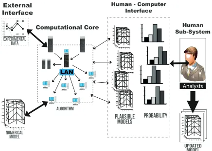
Figure 1.1 Model Updating Cognitive Systems (MUCogS) Framework . . . . 4

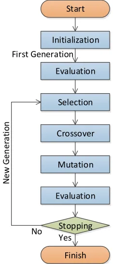
Figure 2.1 Traditional Genetic Algorithm Flowchart . . . 9

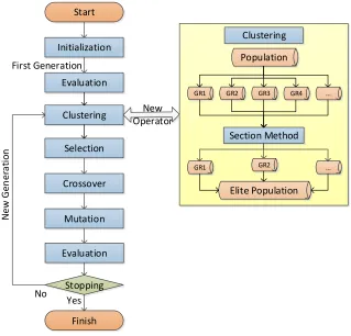
Figure 2.2 Multi-Solution Genetic Algorithm (MsGA) Flowchart . . . 10

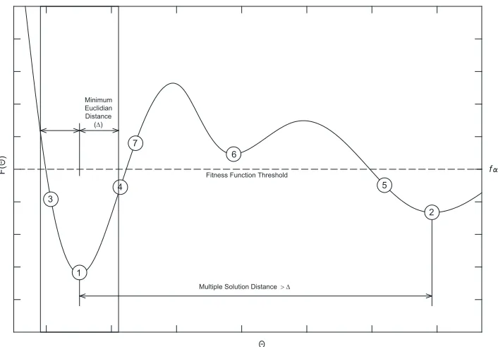
Figure 2.3 Clustering Criteria . . . 12

Figure 2.4 Surface Plot for 2 Parameters . . . 14

Figure 2.5 Possible Multiple Solutions for Run 1 (fα= 1.5 and ∆ = 5%) . . 15

Figure 2.6 Cut between optima 1 and 4 (left) and optima 1 and 7 (right) . . 16

Figure 2.9 Condor Framework . . . 21

Figure 2.10 Condor Speed Test without Delays . . . 23

Figure 2.11 Condor Speed Test with Delays . . . 24

Figure 2.12 High Throughput Multi-Solution Genetic Algorithm (HTMGA) Flowchart . . . 25

Figure 3.1 Multiple Solutions for Equation (3.1) . . . 28

Figure 3.2 Multiple Solutions for Equation 3.2 . . . 30

Figure 3.3 Multiple Solutions for Equation 3.2 with Populations of 50,100, 200, 500, 1000, 2000, 5000 . . . 30

(12)

Figure 3.5 Multiple Solutions for Equation 3.2 with 5, 10, 15, 20, 25, 30,

50 Mutation Percentages . . . 33

Figure 3.6 Plot for Number of Solutions for Equation 3.2 with Mutation Percentages of 5, 10, 15, 20, 25, 30, 50 . . . 35

Figure 4.1 Illustrative Test Structure . . . 37

Figure 4.2 Experimental Mode Shapes for First 5 Frequencies . . . 40

Figure 4.3 Numerical Mode Shapes for First 5 Frequencies . . . 42

Figure 4.4 Modular Test Structure . . . 44

Figure 4.5 Experimental Setup . . . 46

Figure 4.6 Amplitude-Frequency Response for Test 1 . . . 47

Figure 4.10 Stabilization Diagram on Amplitude-Frequency Response . . . 51

Figure 4.11 Mode Shapes for Experimental Results . . . 53

Figure 4.12 Numerical Model Setup for Test Structure . . . 54

Figure 4.13 Mode Shapes for Numerical Analysis . . . 58

Figure 4.14 Test Structure with 2 Unknown Parameters . . . 60

Figure 4.15 HTMGA results for 3 sensors . . . 61

(13)

Chapter 1 Introduction

Numerical models of structural systems, such a Finite Element Model, are commonly used to estimate the behavior of existing structures by performing dynamic analysis, stress analysis, and life time prediction among other type of analysis [Cook et al., 2001]. Because of uncertainties in model parameters and modeling errors, analytical model of existing structures do not always accurately represent the structure and up-dating the model might be needed [Brownjohn and Xia, 2000, Brownjohn et al., 2003, Doebling et al., 1996]. For example, Teughels and De Roeck [2004] compared the nat-ural frequencies and mode shapes of a model of the Z24 bridge with experimental data from actual structure. The differences between numerical and experimental natural frequencies were up to 6.82%. Using the original model for an earthquake analysis, for example, could have included significant errors in the results. Model updating is innovative way of modeling structural systems by integrating experimental data into numerical models. Model updating techniques commonly use optimization tech-niques to minimize a function expressing the error between a predicted behavior from the numerical model and observations of the same behavior obtained experimentally. Optimization techniques are used to identify the structural parameters that minimize this error function.

(14)

the extraction of system features from the experimental data and limited number of sensors that cause whether or not the global (best) solution is the best physical representation of the structure. One could argue that a local solution could be a better representation of the parameters of the structure [Caicedo and Zarate, 2011]. Caicedo and Zarate [2011] applied model updating technique for 2 floors building structure to update stiffness of each floor. Two solutions are found; stiffness of each floor are very close for first solution and stiffness of first floor is almost 3 times of second floor for second solution. First solution is physically more meaningful for the structure.

There is also another challenge with optimization technique. Optimization meth-ods usually follow the slope for convergence the solution. Error functions are generally not smooth nor continuous since modal parameters are used and modes switch.

1.1 Model Updating Cognitive System

(15)

shear building requires a minimum number of sensors to be globally identifiable. Furthermore, Zarate and Caicedo [2008] argue that a local minima could have a better physical representation of the structural parameters (e.g. mass, stiffness) given a limited number of sensors. Caicedo and Zarate [2011] shows the existence of multiple solutions in a simple experimental test of a 2DOF shear building.

(16)

Figure 1.1 Model Updating Cognitive Systems (MUCogS) Framework

Similar to other model updating techniques, one of the challenges with MUCogS is the high computational cost to identify plausible solutions. Especially in cases where the number of parameters to be updated is high.

(17)

Multi-objective optimization techniques have also been used for model updating. Jaishi and Ren [2007] use one objective function to measure the error in the natural frequencies and a second function to measure the modal strain energy error. The multi-objective minimization provides the parameters of the updated model.

BRILL et al. [1990] presents the Hop Skip and Jump (HSJ) method as a technique to identify a small number of multiple solutions. The analyst or engineer can make a decision on what solution to accept or reject based on his/her own experience and other information that might not be incorporated in the mathematical model. HSJ was originally used for complex or incompletely defined problems that have no exact solution. The technique was later adapted by Zarate and Caicedo [2008] for model updating of structural systems and applied to the Bill Emerson Memorial Bridge.

1.2 Genetic Algorithms

Genetic Algorithms (GAs) are a popular evolutionary technique used for optimization. This is achieved by encoding the characteristics of several individuals in a "chromo-some" or "genome" and mimicking the evolutionary process to find an individual with best fit.

Genetic Algorithms for global optimization problems have been used in many different type applications of engineering optimization such as the calibration of rain-fall–runoff models [Cheng et al., 2005], discrete optimization of structures [Rajeev and Krishnamoorthy, 1992], sizing, shape and topology design optimization of trusses [Ra-jan, 1995], optimized design of two-dimensional structures [Camp et al., 1998], struc-tural topology optimization [Jakiela et al., 2000] and strucstruc-tural damage detection [Chou and Ghaboussi, 2001].

(18)

optimization of trusses. Optimization of sizing, shape and topology are considered both as continues and discrete variables for design of truss structures. Camp et al. [1998] proposes a method combination of a modified Finite Element Analysis Program and Genetic Algorithm for design of discrete structural systems. Chou and Ghaboussi [2001] is using genetic algorithm to minimize error between natural frequencies and mode shapes for detection and identification of structural damage.

1.3 Research Contribution

The research proposes a technique that is able to identify alternate solutions in a structural model updating context. Contribution of this research can be listed as below:

• Study if limited number of sensors create multiple solutions in deterministic model updating.

• Propose and validate a technique to find multiple solutions.

(19)

Chapter 2 High Throughput Multi-Solution Genetic

Algorithm

High Throughput Multi-Solution Genetic Algorithm (HTMGA) is a modified genetic algorithm specifically designed to identify local minima in a high throughput com-puting. HTMGA is created by adding and modifying some operators in traditional genetic algorithm.

HTMGA is proposed to deal with several challenges with the current state of the art in model updating techniques. One of the challenges is the high computational time required to update structural models because the number of parameters to be updated is usually high. Another challenge is whether or not the global (best) solution is the best physical representation of the structure. Most model updating techniques are interested in finding the global minima of the error function. However, one could argue that due to modeling errors and other factors, a local minima could provide a solution with parameters that are more physically meaningful with a slightly reduction on the value of the error function.

2.1 Genetic Algorithm

(20)

of real numbers. HTMGA has been developed based on a real gen, enabling the application of the technique for model updating of structural systems.

(21)

Start

Initialization

Evaluation

Selection

Crossover

Mutation

Stopping

Finish First Generation

N

ew

G

en

er

at

io

n

No Yes Evaluation

Figure 2.1 Traditional Genetic Algorithm Flowchart

2.2 Cluster Operator

(22)

Start Initialization Evaluation Selection Crossover Mutation Stopping Finish First Generation N e w G e n e ra ti o n Population

GR1 GR2 GR3 GR4

Section Method

...

GR1 GR2 ...

Elite Population Clustering

Clustering _OperatorNew

No Yes Evaluation

Figure 2.2 Multi-Solution Genetic Algorithm (MsGA) Flowchart

New clusters are assigned if the i-th individual considered comply with two criteria: minimum Euclidean distance (∆) and fitness function threshold (fα). The minimum

(23)

better fitness function.

The fitness function threshold is used to limit the fitness value of new local optima. To illustrate the fitness function threshold consider the functionf(θ) shown in figure 2.3 and assume that a minimization is being performed. The value of the fitness function threshold is defined after each generation using:

fα =f1+α(fl−f1) (2.1)

where f1 is the fitness function for the global optima and α is a constant defined

by the user. In cases where the fitness function has a physical meaning the analyst can specify a set value for fα instead of using Eq.2.1. This definition of fα was

selected over fα = αf1 because optimization problems where the global minima is

zero would result in no alternate solutions. The number inside each circle (figure 2.3) indicates the location of the individual after sorting them using the fitness function. The fourth individual (Λ4) is not considered the lead of a new group because the

Euclidean distance to Λ1 is less than ∆. However, Λ6 becomes the lead of a new

group because f6 ≤fα and kθ6 −θ1k ≥ ∆, where k: k indicates Euclidean distance

(24)

1 3

7

6

5

2 4

F(

)

Minimum Euclidian Distance (∆)

Fitness Function Threshold

Multiple Solution Distance > ∆

f

Figure 2.3 Clustering Criteria

2.3 Section Method

(25)

while increasing the computation time.

2.4 Numerical Validation

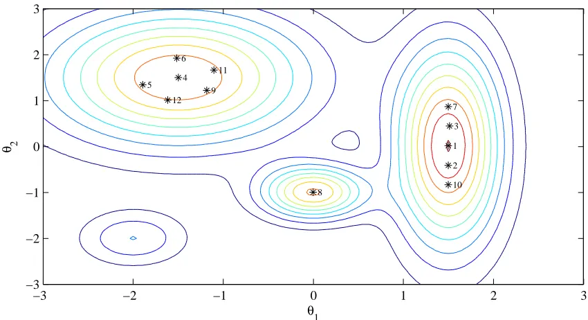
This section implements the MsGA to a close form two variable function for validation purposes. A two variable function is used here to able to plot the values of the objective function and verify that the method is working correctly. The function used for validation is obtained by a combination of Gaussian-like functions defined by the equation:

f(θ1, θ2) = 4 X

i=1

hi×e

[1₂

_θ

1−µ₁,i

σ₁_,i

2

−1 2

_θ

2−µ₂,i

σ₂_,i

2

]

(2.2) The location of the peaks and their shapes are defined by the matrices

µ=



  

1.5 0 −1.5 −2 0 −1 1.5 −2

    ;σ =    

0.4 0.4 1 0.4 1.5 0.4 1 0.4



  

The amplitude for each peak is modified by the constants

h=

2 1.6 1.8 0.6

.

(26)

−4

−2

0

2

4 −4

−2

0

2

4

0

1

2

3 θ

₁

θ

₂

f(

θ

1

,

θ

2

)

Figure 2.4 Surface Plot for 2 Parameters

First, the maximum fitness threshold (fα) is chosen as 1.5 and the minimum

(27)

Table 2.1 Possible Multiple Solutions for Run 1 (fα = 1.5 and ∆ = 5%)

No f(θ1, θ2) θ1 θ2

1 2.0066 1.4983 0.0150 2 1.9306 1.4980 -0.4093 3 1.9244 1.5116 0.4443 4 1.8000 -1.5000 1.5000 5 1.6448 -1.8939 1.3414 6 1.6451 -1.5153 1.9240 7 1.7075 1.4971 0.8690 8 1.6273 -0.0026 -0.9934 9 1.6451 -1.1817 1.2194 10 1.7164 1.4971 -0.8336 11 1.6411 -1.1024 1.6638 12 1.5842 -1.6153 1.0079

1 2 3 4 5 6 7 8 9 10 11 12 θ₁ θ 2

−3 −2 −1 0 1 2 3

(28)

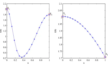
Figure 2.6 shows two sample sections. The cut or section between solution 1 (S1)

and solution 4 (S4) shown on the left and cut between solution 1 (S1) and solution 7

(S7). First, a unit vector between S1 and S4 is calculated by using:

uS1−S4 =

θS4 −θS1

kθS4 −θS1||

(2.3)

whereuS1−S4 is the unit vector betweenS1 andS4,XSi is the vector of parameters of

the i-th possible solution and k: k indicates norm. Points between the two possible solutions can be obtained using the equation:

Xn=XS1 +n×uS1−S4 × kθS4 −θS1|| (2.4)

where n is a number between zero and one.

0 0.2 0.4 0.6 0.8 1

0.2 0.4 0.6 0.8 1 1.2 1.4 1.6 1.8 2 2.2 S 1 S 4 n f( θ )

0 0.2 0.4 0.6 0.8 1

1.7 1.75 1.8 1.85 1.9 1.95 2 2.05 2.1 S 1 S 7 n f( θ )

Figure 2.6 Cut between optima 1 and 4 (left) and optima 1 and 7 (right)

(29)

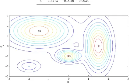
minimum Euclidean distance criterion for this test. This emphasizes the importance of these two parameters. Ideally the analyst will have an idea about what distance would be appropriate for two solutions to be considered physically different. For example, within the context of model updating of structural systems a change of mass or stiffness of more than 15% could be significant.

No f(θ1, θ2) θ1 θ2

1 2.0066 1.4984 0.0107 2 1.8000 -1.5000 1.5000 3 1.6273 -0.0026 -0.9934

1 2

3

θ₁ θ 2

−3 −2 −1 0 1 2 3

Figure 2.7 Possible Multiple Solutions for Run 2 (fα = 1.5 and ∆ = 15%)

(30)

No f(θ1, θ2) θ1 θ2

1 2.0066 1.4984 0.0107 2 1.8000 -1.5000 1.5000

1 2

θ

1

θ 2

−3 −2 −1 0 1 2 3

Figure 2.8 Possible Multiple Solutions for Run 3 (fα = 1.5 and ∆ = 25%)

2.5 High Throughput Computing

(31)

been proposed for this problem. For example, Cheng et al. [2005] proposes a method that uses a modified GA called Parallel Genetic Algorithm (PGA). PGA works with a fuzzy optimal model in a cluster of computers by creating subpopulations and using additional operators from traditional GA such as migration. PGA needs multi-criteria to create correlations between subpopulations for the selection and evaluation steps. The Java Parallel Virtual Machine(JVPM) is used to implement the algorithm in a distributed computing environment. However, the technique focuses on identifying the global minima (or maxima) of the objective function and does not consider local solutions.

Previous work by Caicedo and Yun [2011] developed two new operators for genetic algorithms based on the concept of MGA. The first operator calculates the MGA solutions each generation. The second operator uses the identified MGA solutions to divide the population in groups. The MGA solutions are identified based on the angle between the hyper-dimensional vectors describing each solution. The time required to find multiple solutions is significant because the algorithm was implemented for a single computer core. In addition, looking at the angles between the vector of solutions could result on missing some solutions that are physically separately in the solution space (e.g.(1,1) and (1e4, 1e4) have the same direction cosines but very different magnitudes).

Computers with several cores are common today and distributing the load between the cores reduces the time that the analyst should spend to run algorithms. Further-more, High-throughput computing (HTC) environments such as Condor [Thain et al., 2005] and Portable Batch System (PBS) (http://www.pbspro.com/) can be used to utilize idle computer time from several CPUs. HTC environment provides a user maximum computational power by taking all the available computing resources in a network [Thain et al., 2005].

(32)

perfor-mance of MsGA is studied in this section. There are three main challenges associated with the use of HTC for MsGA:

• The evaluation of fitness function is computationally expensive for large struc-tural systems.

• HTC environment is heterogeneous (performance of each worker is different).

• Interprocess communication is not allowed in HTC.

(33)

Figure 2.9 Condor Framework

(34)

(35)

0 200 400 600 800 1000 1200 1400 0

10 20 30 40 50 60

Jobs

0 200 400 600 800 1000 1200 1400

0 20 40 60 80 100

Execution Time (sec)

Jobs(%)

(36)

0 1000 2000 3000 4000 5000 6000 7000 8000 0

50 100 150 200 250 300

Jobs

0 1000 2000 3000 4000 5000 6000 7000 8000

0 20 40 60 80 100

Execution Time (sec)

Jobs(%)

Figure 2.11 Condor Speed Test with Delays

(37)

finished within the completion rate are considered for later populations. Setting up the completion rate to the correct value should keep the condor pool with enough running jobs even between populations. This is, some fitness functions should be evaluated while HTMGA prepares the next generation.

Start Initialization Evaluation Selection Crossover Mutation Stopping Finish First Generation N e w G e n e ra ti o n Population

GR1 GR2 GR3 GR4

Section Method

...

GR1 GR2 ...

Elite Population Clustering Clustering No Yes Population

Pop1 Pop2 Pop3 Pop4 ...

Job Manager Evaluation

(38)

Chapter 3 Validation

HTMGA is particularly powerful when functions with a large number of parameters are optimized. However, the visualization of these functions is difficult. This chapter uses a number of multi variable functions to test the capabilities of HTMGA. In a model updating context the location of the optimal solutions are not known. However, before applying the proposed algorithm in this context, it should be validated. This is performed by using a number of functions with known number and location of solutions. This chapter is not intended as a guide to determine the optimal value of the parameters for HTMGA but as a documentation that the algorithm has been tested with a number of functions. First, HTMGA is tested with functions of one and two variables for easy visualization of the results and validation of the technique. In a model updating, the first function used here to study the performance of HTMGA is defined by the following equation:

(39)

Table 3.1 Parameters for HTMGA to Run One Variable Function Options

Optimization Type Max. Population Size 100 Number of Variables 1 Variable Limits [0 1] Max. Generations 100 Elite Population 5% Mutation Population 15% Mutation Limit 15% Minimum Euclidean Distance 5% Fitness Limit 0.90

(40)

0 0.1 0.2 0.3 0.4 0.5 0.6 0.7 0.8 0.9 1 0

0.2 0.4 0.6 0.8 1 1.2 1.4

θ

f(

θ

)

Figure 3.1 Multiple Solutions for Equation (3.1)

HTMGA can also detect a large number of multiple optima values. Arguably, in a model updating context only a limited number of plausible solutions is preferred because it would help the analyst decide the most appropriate parameter values. However, it is worth testing the algorithm with functions that have several optimal values from an algorithm development point of view. The second function used in this chapter has a total of 100 solutions and it is defined by the equation:

f(θ1, θ2) = sin(19×πθ1) +

θ1

1.7 + sin(19×πθ2) +

θ2

(41)

Table 3.2 Parameters for HTMGA to Run Two Variable Function Options

Optimization Type Max. Population Size 5000 Number of Variables 2

Variable Limits [0 1; 0 1] Max. Generations 100 Elite Population 5% Mutation Population 15% Mutation Limit 15% Minimum Euclidean Distance 5% Fitness Limit 0.90

whereθ1 and θ2 are the parameters of the function. The options for the algorithm

(42)

θ₁ θ 2

0 0.1 0.2 0.3 0.4 0.5 0.6 0.7 0.8 0.9 1

Figure 3.2 Multiple Solutions for Equation 3.2

0 0.2 0.4 0.6 0.8 1 0

0.5 1

θ₁

θ 2

0 0.2 0.4 0.6 0.8 1 0

0.5 1

θ₁

θ 2

0 0.2 0.4 0.6 0.8 1 0

0.5 1

θ₁

θ 2

0 0.2 0.4 0.6 0.8 1 0

0.5 1

θ₁

θ 2

0 0.2 0.4 0.6 0.8 1 0

0.5 1

θ₁

θ 2

0 0.2 0.4 0.6 0.8 1 0

0.5 1

θ₁

θ 2

0 0.2 0.4 0.6 0.8 1 0

0.5 1

θ₁

θ 2

Figure 3.3 Multiple Solutions for Equation 3.2 with Populations of 50,100, 200, 500, 1000, 2000, 5000

(43)

etc) indicates the results of a different run. The results are summarized in table 3.3. As expected, the number of solutions found decreased with small populations. Since the algorithm uses clusters the population method, population size is divided in small groups. If the number of groups is too high, the number of individuals for each group is very low. In this case, even though more solutions can be obtained with high number of generation, some solutions can be inaccurate if a small number of generations is used (table 3.4). Usually, there is an inverse correlation between the number of generations and the population size in traditional genetic algorithm. However, when multiple solutions are considered, there is also a direct correlation between the expected number of solutions and population size. A logarithmic correlation was found for this particular example (figure 3.4).

Table 3.3 Number of Multiple Solutions are found with 50,100, 200, 500, 1000, 2000, 5000 Population Size

Population

Size

(44)

Table 3.4 Number of True and False Solutions are found with Distance<0.015

Population

Size

Number of Solutions Found

Run-1 Run-2 Run-3 Run-4 Run-5 T F T F T F T F T F 50 5 26 8 22 13 19 7 26 7 23 100 39 11 33 12 33 14 35 8 33 12 200 57 2 57 1 56 1 53 3 47 8 500 77 0 72 0 76 0 69 1 77 0 1000 92 0 91 0 91 0 92 0 91 0 2000 99 0 100 0 96 0 98 0 97 1 5000 100 0 100 0 100 0 100 0 100 0

0 500 1000 1500 2000 2500 3000 3500 4000 4500 5000 0

10 20 30 40 50 60 70 80 90 100

Individuals

Number of Solutions

Figure 3.4 Plot for Number of Solutions for Equation 3.2 with Populations of 50,100, 200, 500, 1000, 2000, 5000

(45)

algo-rithm is expected to focus on the first (or few first) solutions found. In contrast, if the mutation percentage is too high, the algorithm could take many generations to find accurate results. HTMGA was tested with a number of mutation percentages in-cluding 5, 10, 15, 20, 25, 30, 50 percent. The number of solutions identified changed depending on the percentage of the population that was mutated each generation (figure 3.5). Table 3.5 shows the number of solutions that the algorithm reported (regardless of whether they were correct or not) for different values of mutation per-centage. Higher mutation percentage yielded a higher number of solutions; however it causes higher computation time. Table 3.6 shows how many of the solutions are correct. In general only one or zero solutions were found to be inaccurate, indicating that the mutation percentage has little effect in the accuracy of the solution. Figure 3.6 shows a graph of the number of solutions as a function of the mutation percentage. An optimal value for this particular problem seems to be around 35%.

0 0.2 0.4 0.6 0.8 1 0

0.5 1

θ₁

θ 2

0 0.2 0.4 0.6 0.8 1 0

0.5 1

θ₁

θ2

0 0.2 0.4 0.6 0.8 1 0

0.5 1

θ₁

θ 2

0 0.2 0.4 0.6 0.8 1 0

0.5 1

θ₁

θ 2

0 0.2 0.4 0.6 0.8 1 0

0.5 1

θ₁

θ2

0 0.2 0.4 0.6 0.8 1 0

0.5 1

θ₁

θ 2

0 0.2 0.4 0.6 0.8 1 0

0.5 1

θ₁

θ 2

(46)

Table 3.5 Number of Multiple Solutions are found with Mutation Percentages of 5, 10, 20, 25, 30, 50

Mutation

Percentage

Number of Solutions Found Run-1 Run-2 Run-3 Run-4 Run-5

5 32 40 33 34 36

10 37 40 40 43 42 15 79 70 78 76 77 20 71 75 72 73 71 25 85 83 83 81 82 30 88 82 81 82 77 50 93 97 91 90 88

Table 3.6 Number of True and False Solutions are found with Distance<0.015

Mutation

Percentage

Number of Solutions Found

(47)

0 5 10 15 20 25 30 35 40 45 50 0

10 20 30 40 50 60 70 80 90 100

Mutation Percentage (%)

Number of Solutions

(48)

Chapter 4 Application to Model Updating of Structural

Models

Numerical models of structural systems, such a Finite Element Model, are commonly used to estimate the behavior of a structure by performing dynamic analysis, stress analysis, and life time prediction among other type of analysis. Numerical modeling plays a critical role in analysis, design and retrofit of structural systems. Analyt-ical model of existing structures do not always accurately represent the structure and modal updating is necessary because of uncertainties in model parameters and modeling errors.

In this Chapter, model updating of structural models will be performed on an il-lustrated numerical test structure (figure 4.1) and on a modular test structure (figure 4.4) that was designed and built at the Structural Dynamics and Intelligent Infras-tructure (SDII) research group at the University of South Carolina. HTMGA, is used to minimize the error function that describes the differences between the data simu-lated from a numerical model and an equivalent data set collected experimentally.

(49)

There are two types of modal identification: input-output and output-only modal identification. The loads (forces acting in the structure) are not required to be known for output-only methods. Inputs are assumed as stochastic processes with some par-ticular characteristics (e.g. stationary). Output only methods are preferred in struc-tural engineering because it allows modal identification without closing the structure [Van Overschee and Moor, 1996, Van Overschee et al., 1997].

4.1 Numerical Example

Before testing HTMGA on a real structure, an illustrative numerical structure is considered. The test structure is a 5 story shear structure in the XZ plane (figure 4.1). There is a total of 6 nodes on the structure and each node has one degree of freedom in the X direction. The structure is fixed at the base for a total of five degrees of freedom. In this particular application the "real" structure and the model that will be updated will be the same, eliminating modeling errors. Modeling errors will be included in the experimental implementation of the technique later in this chapter.

Figure 4.1 Illustrative Test Structure

(50)

(G), cross section area(A), rotational inertia (J), inertia around the X axis (Ix), etc. are set to values is shown in table 4.1.

Table 4.1 Section and Material Properties for Illustrative Test Structure Section Properties Material Properties

A(mm2₎ ₄₀₆ _E(GPa) _199.9

I(mm4₎ ₃₈₆₄ _ρ₍_kg/m3₎ ₇₈₉₀

J(mm4₎ ₇₇₂₉ _υ₍₋₎ _0.3

The Young Modulus (E) for each column is assumed as unknown for a total of five variables to be updated. The search space is defined with lower limit 0.5*(E) and upper limit 1.5*(E). Model analysis is not required in this example since the values of the natural frequencies and mode shapes are available directly from the stiffness and mass matrix. An Eigenvalue analysis is performed to calculate natural frequencies (eigenvalue) and mode shapes (eigenvector).

The natural frequencies and mode shapes are found by solving the equation:

[K−λ2_iM][Φi] = 0, i= 1,2,3... (4.1)

where λi is the i-th natural frequency and [Φi] is the corresponding mode shapes.

The mass matrix [M] and the stiffness matrix [K] of the illustrated structure are:

[M] =

               

4 0 0 0 0 0 4 0 0 0 0 0 4 0 0 0 0 0 4 0 0 0 0 0 2

(51)

[K] =                

12(E1+E2) −12E2 0 0 0

−12E2 12(E2+E3) −12E3 0 0

0 −12E3 12(E3+E4) −12E4 0

0 0 −12E4 12(E4+E5) −12E5

0 0 0 −12E5 12E5                

×3.864×10−8

where Ei is the young modulus of i-th column. The same stiffness and mass

matrices are used for the "real" or reference model and for the model that will be updated. The value of the natural frequencies and mode shapes for the reference model are shown in tables 4.2 and 4.3 respectively. The mode shapes are shown in figure 4.2 and correspond to the typical mode shapes of a shear building. These model parameters will be considered the "experimental" model parameters.

Table 4.2 Experimental (References) Natural Frequencies Mode Natural Frequency(Hz) 1 7.58

2 22.00 3 34.26 4 43.17 5 47.86

Table 4.3 Experimental (References) Mode Shapes

Mode

Floor

1 2 3 4 5

(52)

Figure 4.2 Experimental Mode Shapes for First 5 Frequencies

After experimental natural frequencies and mode shapes are obtained, the ob-jective (error) function needs to be defined. Usually, the difference between natural frequencies and mode shapes are used as an error function. One of challenges with this strategy is that the mode shapes should be matched before the error function is calculated. This is, to make sure that the mode is compared is the same for the experimental and the numerical model. For example, in this case, the first bending mode shape of the experimental data should be compared with the data from the first bending mode of the numerical model. Some authors put some metrics on the matching of the mode shapes. For example, match modes that have a modal as-surance criteria (MAC) greater than 0.95. Modes that do not have this metric are not considered not matching and are not included in the metric. Here MAC values of more than 0.9 and frequency differences of less than 0.5 are considered a match. The error between the numerical and "experimental" models is calculated using the following equation:

f(O/) =

n

X

frefi−fnumi

fref

+ (1−M AC(O/_ref_i, /O_num_i)

!

(53)

where n is the number of matching modes, frefi is i-th matching mode reference

natural frequency fnumi is i-th matching mode numerical natural frequency O/refi is

i-th matching mode reference mode shape and O/_num_i is i-th matching mode natural frequency. If there is no matching mode, the objective value is set to infinite.

Consider the following case as a demonstration for the calculation of the objective (error) function. First, values for E are randomly chosen, and the stiffness matrix is calculated. This is equivalent to considering an individual from the first generation, where the value of the parameters is chosen randomly. Consider the randomly selected values.

E =

0.82 0.89 1.24 0.52 1.42

[K] =

               

1.5850 −0.8249 0 0 0

−0.8249 1.9743 −1.1494 0 0

0 −1.1494 1.6313 −0.4820 0 0 0 −0.4820 1.7982 −1.3162 0 0 0 −1.3162 −1.3162

               

×105

Natural frequencies (table 4.4) and mode shapes (table 4.5) are calculated by performing Eigen analysis with the original mass matrix and the stiffness matrix shown in Eq.4.2. Mode shapes for each natural frequency are shown in figure 4.3. Table 4.4 Numerical Natural Frequencies

Mode Natural Frequency(Hz) 1 7.03

(54)

Table 4.5 Numerical Mode Shapes

Mode

Floor

1 2 3 4 5

1 -0.10 0.22 0.40 -0.19 0.02 2 -0.19 0.27 -0.02 0.37 -0.05 3 -0.24 0.19 -0.29 -0.26 0.08 4 -0.31 -0.23 0.04 -0.03 -0.31 5 -0.32 -0.29 0.11 0.13 0.53

Figure 4.3 Numerical Mode Shapes for First 5 Frequencies

(55)

Table 4.6 Error for Natural Frequencies a a a a a a a a a a a_a

ωref(Hz)

ωnum(Hz)

7.03 18.46 32.08 45.06 51.40

7.58 0.08 0.59 0.76 0.83 0.85 22.00 2.13 0.19 0.31 0.51 0.57 34.26 3.87 0.86 0.07 0.24 0.33 43.17 5.14 1.34 0.35 0.04 0.16 47.86 5.81 1.59 0.49 0.06 0.07

Table 4.7 Comparison for Mode Shapes

Mac Values For Numerical and

Experimental Mode Shapes

No 1 2 3 4 5 1 1.00 0.02 0.00 0.00 0.07 2 0.03 0.96 0.01 0.00 0.11 3 0.04 0.08 0.83 0.05 0.19 4 0.03 0.02 0.03 0.68 0.34 5 0.02 0.00 0.00 0.15 0.74

(56)

4.2 Experimental Problem

Figure 4.4 Modular Test Structure

Modal Analysis for Test Structure

Test Specimen

(57)

Experimental Setup

(58)

Figure 4.5 Experimental Setup

Experimental Implementation

(59)

used. In this research, the SSI is used as a modal identification technique to find dynamic behavior of test structure.

Transfer functions between the force on the hammer and acceleration at each node of structure are calculated for each test and shown in figure 4.6, figure 4.7, figure 4.8, and figure 4.9.

(60)

(61)

(62)

Figure 4.9 Amplitude-Frequency Response for Test 4

(63)

Figure 4.10 Stabilization Diagram on Amplitude-Frequency Response

The first 10 natural frequencies and damping ratios are shown in table 4.8 and mode shapes are shown in table 4.9. The mode shapes are plotted in figure 4.11. Table 4.8 Natural Frequencies and Damping Ratio

No Natural

Frequencies (Hz)

Damping

Ratio (%)

(64)

Table 4.9 Modal Coordinates

Node

No

Mode

1 2 3 4 5 6 7 8 9 10

(65)

Figure 4.11 Mode Shapes for Experimental Results

Numerical Analysis for Test Structure

Numerical Model Setup:

(66)

Figure 4.12 Numerical Model Setup for Test Structure

Table 4.10 Node Coordinates for Test Structure Node Coordinates

No X(m) Y(m) No X(m) Y(m) No X(m) Y(m) No X(m) Y(m) 1 1.209 0.000 5 0.806 0.000 9 0.403 0.000 13 0.000 0.000 2 1.209 0.830 6 0.806 0.830 10 0.403 0.830 14 0.000 0.830 3 1.209 1.660 7 0.806 1.660 11 0.403 1.660 15 0.000 1.660 4 1.209 2.490 8 0.806 2.490 12 0.403 2.490 16 0.000 2.490

(67)

Table 4.11 Additional Lumped Masses at the Nodes Additional Lumped Masses Nodes Mass(kg)

1,4,13,16 4.94 2,3,14,15 6.42 5,8,9,12 5.74 6,7,10,11 7.52

Table 4.12 Material Properties for Test Structure Material Properties E(Gpa) 199.9

ρ (kg/m3₎ ₇₈₉₀

υ(−) 0.3

Table 4.13 Cross Sectional Properties For Test Structure Section Properties

A(mm2₎ ₄₀₆

Izz(mm4₎ ₃₈₆₄

Iyy(mm4₎ ₃₈₆₄

J(mm4₎ ₇₇₂₉

Numerical Implementation:

(68)

Table 4.14 Natural Frequencies for Numerical Analysis

No Natural

Frequencies (Hz)

(69)

Table 4.15 Mode Shapes for Numerical Analysis

Node

No

Mode

1 2 3 4 5 6 7 8 9 10

(70)

Figure 4.13 Mode Shapes for Numerical Analysis

Model Updating Using HTMGA

This sections describes the implementation of HTMGA in the model updating of the experimental structure. Different subset of models are updated to explore how multiple alternatives change depending on the number of sensors used for modal identification. Notice that the intention on this phase is not to select the best model but to study if HTMGA can identify multiple solutions within a model updating context. The objective function is the same objective function as used in the previous example. The way to match modes is similar as well.

(71)

Evolution of Number of Solutions as a Function of the Number of Sensors

In this section the moment of inertia of the structural elements are combined in two unknown parameters. This is done to easily visualize the results of HTMGA and study how multiple solutions change as different number of sensors are used for model updating. One parameter is used for the moment of inertia of the structural elements parallel to the X axis and a second parameter is used for the moment of inertia of the elements parallel to Y axis. Notice that the elements are circular so only one moment of inertia is used to describe the cross section. In other words, the moment of inertia of any axis of the cross section is assumed to be the same.

(72)

13 9 5 1 2 6

10 14

15 11 7 3

16 12 8 4

Ix Ix Ix

Iy Iy Iy Iy

Figure 4.14 Test Structure with 2 Unknown Parameters

The experimental data that is obtained by 3, 6, 9 and 12 sensors is used for model updating to study how the numbers of sensors affect the number of solutions. This also helps us evaluate the effectiveness of HTMGA in a model updating context by comparing contour plots of the objective function with the minima found by the algorithm.

(73)

data obtained. This is similar to signal aliasing but occurs in the mode shapes (or special aliasing) because only limited number of sensors are used to identify the modes of vibration. The theoretical value is somewhere close to the solution in the middle of figure 4.15.

Table 4.16 HTMGA Results for 2 Variables with 3 Sensors

] Error Ix(mm4₎ _Iy(mm4₎

1 0.0847 3693.3 3669.1 2 0.1177 3665.3 4986.0 3 0.1347 3854.0 2251.1 4 0.1829 2415.4 3693.5

0.084677 _0.11772

0.13473

0.18292

Moment of Inertia(Iy) (*103 mm4)

Moment of Inertia(Iz) (*10

3 mm 4 )

2 2.5 3 3.5 4 4.5 5 5.5

(74)

The next run uses six sensors on nodes 2, 7, 8, 9, 10 and 15. HTMGA results are shown in table 4.17 and figure 4.16. HTMGA successfully identified the two local minima of the objective function. As expected, the number of solutions decreased as more sensors are used for updating. Interestingly, the local minima corresponding to the theoretical solution disappears when more sensors are added. One plausible explanation is that modeling errors are present. In particular, the boundary condi-tions of the numerical model might not match those of the experimental data. The theoretical model allows only rotations along the X axis. Rotations along the Y and Z axis is not allowed. In reality, the structure could allow some rotations about the Y axis. The value of objective function increased when more sensors were used. Table 4.17 HTMGA Results for 2 Variables with 6 Sensors

(75)

0.3799

0.39807

3 mm 4 )

2 2.5 3 3.5 4 4.5 5 5.5

Figure 4.16 HTMGA results for 6 sensors

The next run uses nine sensors on nodes 2, 5, 6, 7, 8, 9, 11, 12, and 14. HTMGA results are shown in table 4.18 and figure 4.17. Once again HTMGA does a good job identifying the local minima. In this case one minimum was found. This minimum is close the local minimum found with six sensors. The objective function is smoother than in the previous cases and the value of the objective function is similar than in the previous run.

(76)

0.34722

3 mm 4 )

2 2.5 3 3.5 4 4.5 5 5.5

Finally, sensors are installed in all nodes that are not in the supports. These are 2, 3, 5, 6, 7, 8, 9, 10, 11, 12, 14 and 15. HTMGA results are shown in table 4.19 and figure 4.18. The results for this run are similar to those found with nine sensors. This indicates that special aliasing for this particular structure does not appears to happen with more than nine sensors installed.

(77)

0.33586

3 mm 4 )

2 2.5 3 3.5 4 4.5 5 5.5

(78)

Table 4.20 Case Studied with 2 Variables

Case Study ]of sensors ] of solutions

1 3 4

2 6 2

3 9 1

4 12 1

Model Updating with 8 Unknown Parameters

(79)

13 9 5 1 2 6

10 14

15 11 7 3

16 12 8 4

Ix1 Ix3 Ix1

Iy1 Iy3 Iy1

Ix2 Ix4 Ix2

Ix1 Ix3 Ix1

Iy2 Iy4 Iy2

Iy1 Iy3 Iy1

Figure 4.19 Test Structure with 8 Unknown Parameters

The aim of testing a different number of sensors is to study if the results improve and behave as in this previous section.

(80)

] Error Ix1 Ix2 Ix3 Ix4 Iy1 Iy2 Iy3 Iy4

1 0.09733 2497.7 3705.6 3943.2 3478.4 3460.2 2100.5 5651.5 3621.0 2 0.1114 2225.7 5656.9 3848.5 4784.4 3313.0 3272.8 5449.0 2610.9 3 0.1836 2186.6 5313.8 3629.5 4688.2 5102.8 4608.6 2189.3 3979.1 4 0.3380 1938.2 5696.3 2020.9 5429.3 3819.6 2210.6 2823.4 3274.7 5 0.4133 5226.4 4017.8 3910.8 3454.8 4726.8 4789.8 2746.1 3606.7

1 0.1287 1954.8 5318.0 1963.7 2849.3 3585.0 2042.1 5409.6 4016.2 2 0.1773 2654.2 3915.8 2998.9 3918.5 3723.0 2104.0 4799.1 4005.8

1 0.1999 2134.1 4760.8 4863.2 3414.2 3512.8 1977.6 5726.1 3517.8 2 0.2618 1939.7 5084.6 2673.9 5724.9 3178.5 2155.0 4758.9 5047.2

1 0.1345 1951.3 5611.7 1945.1 2658.7 3502.3 2234.2 5758.1 3290.6 2 0.243 2947.1 5290.2 2413.5 3242.3 3704.3 2375.6 5623.3 2894.5

(81)

Table 4.25 Case Studied with 8 Variables

Case Study ]of sensors ] of solutions

1 3 5

2 6 2

3 9 2

(82)

Chapter 5 Conclusions

This research is part of the Model Updating Cognitive Systems (MUCogS) framework acknowledges the existing of multiple solutions. Two methods have been proposed in same context, so far. Zarate and Caicedo [2008] reported a family of different solutions using Modeling to Generate Alternatives (MGA), and Caicedo and Yun [2011] proposed the methodology Steady-State GA for MGA (SSGA-MGA), capable of identify multiple solutions. The proposed technique improve upon the previous techniques by clustering the populations in a more different efficient way than with SSMGA-MGA and reducing the time perform the updating by distributing the load on a condor pool. Previous work (Zarate and Caicedo, Caicedo and Yun) focused on finding solutions that were described with perpendicular vectors to ensure that the solutions were physically different. This work uses an Euclidean distance instead of the angle between vectors. This Euclidean distance can help identify solutions that might be different but are described by vectors that are not perpendicular to each other. This is, have the same direction but different magnitudes. Additional to the proposed technique, the existing multiple solutions on a model updating application is studied as the number of sensors used for implementation changes. The proposed technique (HTMGA) was tested using with a numerical example and an experimental structure. The technique was used to study how the solutions change as the number of sensors used in the instrumentation changes. Results show that the global solution is not always the best solution.

(83)

(84)

Chapter 6 Future Work

This research can be expanded based on the following topics:

• In this research, limited sensors are used to demonstrate for existing of multiple solutions in model updating application. The research can be expanded for optimization of sensor location to minimize existing of multiple solutions.

• HTMGA can be applied in a probabilistic framework (finding areas of high probability in a posterior PDF).

• HTMGA parameters can be updated while it is running. For example, popula-tion size or mutapopula-tion percentage could be increased or decreased.

(85)

Bibliography

D. Bhandari, C. A. Murthy, and S. K. Pal. Genetic algorithm with elitist model and its convergence. International Journal of Pattern Recognition and Artificial

Intelligence, 10(6):731–747, 1996.

ED BRILL, JM FLACH, LD HOPKINS, and S RANJITHAN. Mga - a decision support system for complex, incompletely defined problems. Ieee Transactions

on Systems Man and Cybernetics, pages 745–757, 1990. ISSN 0018-9472.

James Mark William Brownjohn, Pilate Moyo, Piotr Omenzetter, and Yong Lu. Assessment of highway bridge upgrading by dynamic testing and finite-element model updating. Journal of Bridge Engineering, 8(3):162–172, 2003.

JMW Brownjohn and PQ Xia. Dynamic assessment of curved cable-stayed bridge by model updating. JOURNAL OF STRUCTURAL ENGINEERING-ASCE, 126 (2):252–260, 2000.

JM Caicedo and GJ Yun. A novel evolutionary algorithm for identifying multiple alternative solutions in model updating. Structural Health Monitoring-an

Inter-national Journal, 10(5):491–501, 2011.

JM Caicedo and BA Zarate. Reducing epistemic uncertainty using a model updating cognitive system. Advances in Structural Engineering, 14(1):55–65, 2011.

C. Camp, S. Pezeshk, and G. Cao. Optimized design of two-dimensional structures using a genetic algorithm. Journal of Structural Engineering, 124(5):551–559, 1998.

(86)

CT Cheng, XY Wu, and KW Chau. Multiple criteria rainfall-runoff model calibration using a parallel genetic algorithm in a cluster of computers. Hydrological Sciences

Journal-Journal Des Sciences Hydrologiques, 50(6):1069–1087, 2005.

J. H. Chou and J. Ghaboussi. Genetic algorithm in structural damage detection.

Computers & Structures, 79(14):1335–1353, 2001.

R.D. Cook, D.S. Malkus, M.E. Plesha, and R.J. Witt. Concepts and Applications of

Finite Element Analysis. John Wiley & Sons, Inc., 4th edition, 2001.

Scott W. Doebling, Charles R. Farrar, Michael B. Prime, and Daniel W. Shevitz. Damage identification and health monitoring of structural and mechanical sys-tems from changes in their vibration characteristics: A literature review. Report LA-13070-MS, Los Alamos National Laboratory, May 1996 1996.

L. J. Eshelman and J. D. Scahffer. Real-coded genetic algorithms and interval-schemata. Foundations of Genetic Algorithms 2, pages 187–202, 1993.

G. Franco, R. Betti, and R. W. Longman. On the uniqueness of solutions for the iden-tification of linear structural systems. Journal of Applied Mechanics-Transactions

of the Asme, 73(1), 2006.

A. Globus, H. Langhirt, and M. Livny. Javagenes and condor: cycle-scavenging genetic algorithms, 2000.

J.H. Holland. Adaptation in Natural and Artificial Systems. MIT Press, 1975.

B. Jaishi and W. X. Ren. Finite element model updating based on eigenvalue and strain energy residuals using multiobjective optimisation technique. Mechanical

Systems and Signal Processing, 21(5):2295–2317, 2007.

M. J. Jakiela, C. Chapman, J. Duda, A. Adewuya, and K. Saitou. Continuum struc-tural topology design with genetic algorithms. Computer Methods in Applied

Mechanics and Engineering, 186(2-4):339–356, 2000.

(87)

Dudy Lim, Yew-Soon Ong, Yaochu Jin, Bernhard Sendhoff, and Bu-Sung Lee. Effi-cient hierarchical parallel genetic algorithms using grid computing. Future

Gen-eration Computer Systems, 23(4):658–670, 2007.

Zbigniew Michalewicz. Genetic algorithmsă+ data structuresă= evolution programs. Springer-Verlagă(Berlin and New York), 3rd rev. and extended edition edition, 1996. ISBN 3540606769.

Bart Peeters and Guido De Roeck. Reference-based stochastic subspace identification for output-only modal analysis. Mechanical Systems and Signal Processing, 13 (6):855 – 878, 1999.

S. Rajan. Sizing, shape, and topology design optimization of trusses using genetic algorithm. Journal of Structural Engineering, 121(10):1480–1487, 1995.

S. Rajeev and C. Krishnamoorthy. Discrete optimization of structures using genetic algorithms. Journal of Structural Engineering, 118(5):1233–1250, 1992.

M. Sanayei, G. R. Imbaro, J. A. S. McClain, and L. C. Brown. Structural model updating using experimental static measurements. Journal of Structural

Engineering-Asce, 123(6), 1997.

D. Schlierkamp-Voosen. Strategy adaptation by competition. In Proceedings of the

Second European Congress on Intelligent Techniques and Soft Computing, pages

1270–1274, 1994.

A. Teughels and G. De Roeck. Structural damage identification of the highway bridge z24 by fe model updating. Journal of Sound and Vibration, 278(3), 2004.

D Thain, T Tannenbaum, and M Livny. Distributed computing in practice: the condor experience. Concurrency and Computation-Practice & Experience, 17(2-4):323–356, 2005.

Peter Van Overschee and Bart L. R. de Moor. Subspace identification for linear

systems : theory, implementation, applications. Kluwer Academic Publishers,

(88)

Peter Van Overschee, B. De Moor, W. Dehandschutter, and J. Swevers. A subspace algorithm for the identification of discrete time frequency domain power spectra.

Automatica, 33(12):2147–2157, 1997.

Alden H. Wright. Genetic algorithms for real parameter optimization. Foundations

of Genetic Algorithms, pages 205–218, 1991.

Relationships Between Prior Experiences, Current Teaching Contexts, and Novice Teachers' Use of Concrete Representation for Mathematics Instruction

University of South Carolina

Scholar Commons

High Throughput Multi-Solution Genetic

Algorithm (HTMGA) for Identification of

Alternate Solutions in a Structural Model Updating

Context

Muslum Kilinc

Dedication

Acknowledgments

Abstract

Table of Contents

List of Tables

List of Figures

Chapter 1

Introduction

Chapter 2

High Throughput Multi-Solution Genetic

Algorithm

−4

−2

0

2

4

−4

−2

0

2

4

0

1

2

3

θ

θ

f(

θ

,

θ

)

Chapter 3

Validation

Chapter 4

Application to Model Updating of Structural

Models

Modal Analysis for Test Structure

Numerical Analysis for Test Structure

Model Updating Using HTMGA

Chapter 5

Conclusions

Chapter 6

Future Work

Bibliography