Mining Rare Item Sets Using both Top Down and
Bottom up Approach
Arnab Kumar Das Asst Professor Dept of Computer Application
GIMT, Guwahati-17
Abstract: Pattern mining is a data mining method that involves finding existing patterns in data. The main objective is to uncover the hidden regularities in the data. Until now most of the research in pattern mining has been exclusively focused on frequent item sets, however in some situation it is interesting to find patterns that are rare instead of frequent or patterns that reflect a negative co relation between items. These patterns are referred to as rare and negative patterns. For example in jewelery sales data, sales of diamond watches are rare however patterns involving the selling of diamond watches could be interesting. Rare items occur rarely but are of special interest as they may highlight exceptional behavior in the data which is likely of interest. This paper propose a method that uses a bidirectional approach in which we are combining both bottom up and top down method to generate non zero rare item set. The bottom-up search starts from 1-itemset and proceeds upto n-1-itemsets as in Apriori while the top-down search starts from n item sets and proceeds down to 1-itemset.The main idea is to use the upward closure property in the bottom-up approach and downward closure property in the top-down search to reduce the number of candidates generated as well as the number of scans over the dataset. Key words: Rare item set, Non zero rare item set, Minimal Rare item set, Rare Association Rule.
1. INTRODUCTION:
Data mining techniques are used to process huge amounts of information in order to extract hidden knowledge to be directly interpreted or exploited to feed other processes. In many cases, data mining techniques are used to discover patterns that can be of interest to a specific domain of application. A pattern is a collection of events/features that occur together in a transaction database. As a matter of fact, different categories of patterns exist, such as sequences, item-sets, association rules and graph patterns, etc. The choice of a technique depends not only on the nature of input data but also depends on what we want to obtain and what view or part of the data we want to be described or represented in a more intelligible and concise way. To filter out the patterns, some criteria are used. The most known criteria are the support and the confidence. While the support represents the number of times a pattern occurs in the initial database, the confidence represents a proportion value that shows how frequently a part of the pattern, called premise, occurs among all the records containing the whole rule body. Here, we classify pattern categories according to the specific use of the support threshold. In fact, by setting ranges for the support, one can obtain different categories of patterns. For example, if we set a minimum support threshold that a pattern has to satisfy to be considered as an
interesting pattern, we obtain what is called frequent pattern. By setting a maximum support threshold we obtain another category of patterns called rare patterns. Whereas frequent patterns focus on mining patterns that appear more frequently in the database, rare patterns aim at discovering patterns that are less frequent. Rare patterns can be used in different domains such as biology, medicine and security etc.. For example, by analyzing clinical databases one can discover rare patterns that will help doctors to make decisions about the clinical care. In the security field, normal behavior is very frequent, whereas abnormal or suspicious behavior is less frequent. Considering a database where the behavior of people in sensitive places such as airports are recorded, if we model those behaviors, it is likely to find that normal behaviors can be represented by frequent patterns and suspicious behaviors by rare patterns. Each category of patterns explores the data seeking for a specific kind of knowledge. It is noteworthy that other categories of patterns different from frequent and rare patterns can be mined. For example, one can be interested by the patterns with a frequency smaller that an upper limit and greater than a lower limit. Those categories of patterns may be used to answer questions such as what items/objects/products/events are visited/bought/occurred together with a minimum and/or maximum frequency. However, some questions may not be directly answered by the mentioned categories of patterns. For instance, with frequent and rare patterns someone may not find the collections of items/objects/products/events that are not visited/bought/occurred together. Answering such questions may be of interest in cases where we are more interested in what is missing than what is already existing, or what we already know about the existing data. Such patterns, we call here as non-present patterns, may potentially be used to detect what is missing in a defective process/situation and correct it by supplying us with candidate solutions that have not yet been encountered.
2.RARE OR INFREQUENT PATTERNS
Patterns that are rarely found in database are often considered to be uninteresting and are eliminated using the support measure. Such patterns are known as infrequent patterns .
items, which are items that can be substituted for one another. Examples of competing items include tea versus coffee, butter versus margarine, regular versus diet soda, and desktop versus laptop computers.
Some infrequent patterns may also suggest the occurrence of interesting rare events or exceptional situations in the data. For example, if {Fire = Yes} is frequent but {Fire = Yes, Alarm = On} is infrequent, then the latter is an interesting infrequent pattern because it may indicate faulty alarm systems. To detect such unusual situations, the expected support of a pattern must be determined, so that, if a pattern turns out to have a considerably lower support than expected, it is declared as an interesting infrequent pattern.
3. BASIC CONCEPTS
We assume standard pattern mining settings, i.e., a set of m items I = {i1, i2, ・・ ・, im} and a transaction database
(TDB) D = {t1, t2, ・・・, tn} on top of I. A subset X of I
is referred to as item set whereby if |X| = k, then X is a k-item set. Moreover, a transaction t is made of an item set I and a unique identifier tid, typically, a natural number. The fraction of transactions in D that contains an item set X is called the (absolute) support of X and is denoted by supp(X) = |{t|t ∈ D,X ⊆ Xt}|. Support is a prime measure of interest for item sets: one is typically – but not exclusively – interested in regularities in the data that manifest in recurring patterns. Thus, intuitively, the itemsets of higher support are more attractive.
In this section we present an example of rare and non-present item-set mining. The input data is composed of a database of transactions, and each transaction is identified by an id and composed of a set of items. In the real world, a transaction may be seen as the basket bought by a customer during a determined period of time (day, week, month, etc.). Each basket is composed of a set of items that are purchased together. In Table 1 we represent an abstract database, denoted by P, where the alphabet letters are considered as items. Given the database of transactions such as presented in Table 1, our goal is to find two categories of sets of items, also called item-sets. The first category is composed of item-sets that are present in at most two transactions, and the second category is composed of item-sets that do not occur in any transaction and composed of a maximum number of items equal to the cardinality of the largest transaction. The number of times an item-set occurs in the database is called the item-set support. In our case the minimum support is equal to 3.
Table 1. Transaction Database P
The set of all item-sets that can be generated from the transaction database is presented in Figure 1 by a diagram
of the subset lattice for five items with the associated frequencies in the database. In the lattice each level is composed of item-sets having the same length. The top element in the lattice is the empty set.
Figure 1. Lattice representing a hierarchically ordered space of item-sets and their frequencies. Frequent item-sets
are square-shaped, rare item-sets are oval-shaped and non-present item-sets are diamond-shaped.
Each lower level k contains all of the item-sets of length k, also denoted k-sets and the last level contains an item-set composed of all items (i.e. a, b, c, d, e). Lines between nodes represent a subset relationship between item-sets. For each item-set we compute its support. For example, the item-set composed of the items b and d denoted by <bd> have 2 as support, and we denote it by <bd,2>. In fact, the item-set bd is present in the transactions t1, t2. The set of rare item-sets we are looking for are those in the lattice with support greater than 0 and less than 3. The rest of item-sets are either frequent (having support greater or equal to 3) or non-present (support=0). In Figure 1 rare item-sets are drawn with ovals, frequent item-sets are drawn with rectangles where non-present item-sets are drawn with diamonds. Thus, after counting the frequencies of each set, we obtain the following set of rare item-sets <e,2>, <ad,1>, <ae,1>, <bd,2>, <be,1>, <cd,2>,<cd,2>, <de,1>, <abd,1>, <abe,1>, <acd,1>, <ace,1>, <ade,2>, <bcd,1>, <bce,1>, <cde,1>, <abcd,1>, <acde,1>. The set of non-present item-sets is composed of the following elements <abde, 0>, <abce,0>, <bcde,0>, <abcde,0>.
3.1 SOME PROPERTIES AND DEFINTION RELATED TO AN ITEMSET
Monotonicity: If X is a subset of Y then Sup(x) must not exceed Sup(Y). I.e. For all X, Y€J: (X is a subset of Y) f(X) ≤ f(Y).
Anti monotone: If X is a subset of Y then sup(Y) must not exceed sup(X).I.e. For all X, Y€J: (X is a subset of Y) f(Y) ≤ f(X).
Downward Closure property: Any subset of a frequent set is a frequent set
Upward Closure Property:Any superset of an infrequent set is an infrequent set
Definition 1: An item set is a maximal frequent item set (MFI) if it is frequent but all its proper supersets are rare. Definition 2: An item set is a minimal rare item set (mRI) if it is rare but all its proper subsets are frequent.
Definition 3: An item set X is a (minimal or key) generator if it has no proper subset with the same support (∀Y ⊂ X, supp(X) < supp(Y)).
Definition 4: A minimal zero generators (mZG) is a zero item set whose proper subsets are all non-zero item sets.
4.RELATED WORK
The previous methods to mine item-sets can be divided into two categories, namely frequent item-set mining and rare item-set mining techniques. Whereas the problem of frequent item-set mining have been widely studied, the problem of rare item-set mining has just started to spark the researchers interest and non-present item-sets have not yet been addressed as independent mining task.
4.1 Frequent Item-set Mining
Item-set space has two properties, a monotone property and an anti-monotone property [12][2] [20]. Every non-empty subset of a frequent item-set is a frequent item-set, and every superset of a non-frequent item-set is non-frequent. Based on those properties, the algorithm Apriori [2] was developed to efficiently mine frequent item-sets. Later on, new algorithms have been proposed to mine frequent item-sets such as Eclat [24], FP-Growth [11] and TM [19]. A recent survey on frequent item-sets mining techniques is presented in [23]. The Apriori approach was successfully used to generate frequent item-sets contained in a transaction database [2] [3] [17]. Apriori approach exploits the monotonicity property of the
support of item-sets. Apriori-based algorithms perform top-down breadth-first search through the space of all item-sets. In the first pass, the support of each individual item is counted, and the frequent ones are inserted to the frequent item-set set of level 1. In each subsequent pass, the frequent item-sets determined in the previous pass are used to generate new item-sets called candidate item-sets. The support of each candidate item-set is counted, and the frequent ones are determined. This process continues until no new frequent item-sets are found.
4.2 Rare and Non-Present Item-sets
Recently, a work presented in [21] proposes an approach to mine rare item-sets that is based on the Apriori algorithm used to mine frequent item-sets. The main idea consists at traversing the item-set space by the Apriori algorithm used to mine frequent item-sets and collect at each level the item-sets that are usually pruned out in the original algorithm and are used as seed for a second algorithm in order to mine the remaining rare item-sets. Another algorithm, called MINIT, is proposed in [10] to mine only minimal infrequent sets. A minimal infrequent item-set is an infrequent item-item-set that do not have a subitem-set of items which forms an infrequent
item-set. In other words, an infrequent item-set is minimal if all its proper subsets are frequent. It is noteworthy that the output of this algorithm may be used to mine all rare
item-sets. More recently in [1] a framework is proposed that absorbs the spirit of the Apriori approach to tackle the problem of rare item-set mining. In this work, we started by factorizing the key elements of Apriori approaches such as the traversal of the item-set space, the pruning principle, the combination of item-sets at a level to generate new item-set in the next level, and then proposed an Apriori generalized framework that abstracts those elements. However, in the International Journal on Soft Computing, Artificial Intelligence and Applications proposed approach, no distinction is made between rare and non-present patterns. A performance comparison of our algorithm with the algorithm presented in [21] is also presented. Various algorithms are proposed to find rare item set from a large dataset.
4.3 Intrusion Detection
Intrusion detection methods are of two types: anomaly detection and misuse (signature) detection. While anomaly detection techniques focus on the detection of user behaviour that is considered as abnormal [5] [22] [7], signature detection focuses on the identification of a behaviour that is similar to known cases that are considered as intrusions. A model is generally is used to represent the known intrusions [13] [16]. The main drawback of model based intrusion detection is the new attacks may be missed if not always kept up-to-date. In order to overcome this limitation, data mining and machine learning approaches are is the current trend
to detect intrusion [14] [6] [4] [8] [25].
5. EXISTING RARE ITEM SET GENEARTION ALGORITHM: Apriori-Rare[20]: This algorithm generates the frequent as well as rare itemsets. It is a slight modification of Apriori algorithm to generate frequent and rare itemsets.
In Apriori algorithm the rare items are pruned out but here the rare items are also collected along with the frequent item set based on the minimum support value. However, it fails to find all the rare itemsets.
Apriori-Inverse[10]: This algorithm determines only the sporadic rules using one Minsup value and one Maxsup value. The sporadic rules have the property that they fall below user define Maxsup but above the Minconf value. The main advantage of Apriori-Inverse is that it can find the sporadic itemsets much more quickly than apriori. However, a major limitation is that it is incapable of finding all the rare itemsets.
MRG-Exp: This algorithm takes the dataset and min support as input and produces the minimal rare generator as output. This algorithm uses the concept of predecessor support of an item set (i) which is the minimum of the supports of all
ARIMA (Another Rare Item set Miner Algorithm)[19]: This algorithm takes the dataset and minimal rare item set(MRI) as input and produces all non zero rare item set plus minimal zero generator. For this it initially calls the Apriori-Rare or MRG-Exp algorithm that generates the Minimal Rare Item sets. It first consider the smallest minimal rare generator and from this its supersets are generated. A dataset scan is made to check the presence of zero generators and is copied to the minimal zero generator (mRG) set which ultimately reduce the search space. The main advantage of ARIMA is that it can find all rare item set . However, it is dependent on two the algorithms MRG-Exp and Apriori-Rare for the minimal rare item set.
6.DISCUSSION AND MOTIVATION
After studying and analyzing the above mentioned rare item set generation algorithms it is observed that all the above mentioned algorithms have some limitations. The algorithm Apriori-Rare, Apriori- Inverse and MRG-exp are unable to generate all rare item sets. Moreover it is unable to prune the zero rare item set . Although the algorithm ARIMA is capable of generating all rare item set it is dependent on either Apriori-Rare or MRG-Exp. Also the rule generated from this item set is not all interesting. To overcome the limitations faced by the above mentioned algorithms we propose an algorithm which follows a bidirectional approach and takes the min support and dataset as input and produces non zero rare item sets as output. In this algorithm in each pass in addition to counting the supports of the candidates in the bottom up direction it also counts the support of some item sets in the top down direction . We call these item sets as non zero rare item set. This process helps in pruning the candidate set very early in the algorithm. It uses the upward closure and downward closure properties of item set for pruning candidate sets, thereby reducing the computation time considerably. In this algorithm we have mainly used the following properties of an item set.
6.1 Properties of Rare item set
Property 1: If X is a rare item set then all its supersets are also rare item set.
Property 2: If X is non zero item set then all its subset will also be non zero item set.
Property3: If X is a zero rare item set then any superset of it is also a zero rare item set
Property4: If X is a subset of Y and sup(X) =sup(Y) then any subset of Y which contain X will also have the same support as that of X and Y.
The above properties can be used to derive the following theorems
Theorem1: Property 1 and Property 2 can be combined to conclude that if a nonzero rare item(X) in the bottom up direction is a subset of the longest nonzero rare item(Y) in the upward direction then any subset of the longest nonzero rare item(Y) which contains X will also be nonzero rare items.
Theorem2: If a zero rare item(X) in the bottom up direction is a subset of the longest zero rare item(Y) in the
upward direction then any subset of the longest zero rare item (Y) which contains X will also be zero rare items. Theorem3: Property 4 can be used to conclude that if a rare item(X) in the bottom up direction is a subset of the longest zero rare item(Y) in the upward direction and both having the same support then any subset of the longest zero rare item (Y) which contains X will also have the same support as that of X and Y.
7.PROPOSED ALGORITHM FOR MINING NON ZERO RARE ITEM SET
1. L0 = ; k=1
2. C1={{i}| i € I}
3. NZRCS = {1, 2 ...n} 4. NZRS=
5. While (ck≠)
6 .Read dataset to count the support of item set in ck and
NZRCS
7. NZRS=NZRS U {non zero rare item set in NZRCS} 8. Lk= {frequent item set in ck }
9. ZRk= {zero rare item set in ck }
10. NZRk= {non zero rare item set in ck }
11. NZR=U NZRk
12. Call the fjoin procedure to generate Ck+1 using NZRk U
Lk
13. Call the NZRCS generation procedure 14. Call the NZRCS update procedure 15. k=k+1
16. Return NZRS
NZRCS generation procedure {
Remove all elements in NZRCS with support ≥ min support
For all item set s € NZRCS with |s|=L do
If(sup(s)==0) then
Remove s from NZRCS and add all (L-1) subset of s to NZRCS
Else
Add s to NZRS and all subset of s that contain an item in NZR as its subset if it is not already there , otherwise add (L-1) subset of s to NZRCS
Update NZRCS using element from ZRk
}
Update NZRCS (NZRCS, ZRk)
{
For all item sets s € ZRk do
For all item sets m € NZRCS do If s is a subset of m then
NZRCS=NZRCS – {m}
For all items e € s
If m-{e} is not a subset of any item set in NZRCS
NZRCS=NZRCS U {m-{e}} End
End End
7.1 Description of the algorithm
In the proposed algorithm if an item set is found to be infrequent in the bottom up direction then this can be used to find non zero rare item set provided it is a subset of a non zero rare item set in the top down direction. i.e. If any subset of non zero rare items in the upward direction contains an infrequent item from the downward direction then those sub item sets are also a nonzero rare item set. This approach not only reduces the number of candidate item set but also minimizes the number of dataset scan required compared to other rare item set generation algorithm. Another property of a rare item set is that if a zero rare item in the bottom up direction is a subset of the longest zero rare items in the upward direction then any subset of the longest zero rare which contains the zero rare item in the bottom up direction will also be zero rare items. This information can be used to prune the zero rare items as we are only interested to mine non zero rare items.
The proposed algorithm takes the dataset and minimum support as input and produces non zero rare item set as output.
In this algorithm we have maintained the following list CK = Candidate item set containing K items generated
using NZRk-1 U Lk-1
ZRk=Zero rare item set in CK
NZRk=Non zero rare item set in CK
NZR=
K K
NZR
Lk=Frequent item set in CK
NZRCS=Non zero rare candidate set which will initially contain all elements in the dataset
NZRS= Non zero rare item set which will initially contain NULL
In the initial step it makes a scan of the dataset to find the support count of the itemset in Ck and NZRCS and divide
the items in the following category as follows
Zero rare items: Items having support count equal to zero.
Frequent items: Items having support count greater or equal to minimum support
Non zero rare items:Items having support count less than minimum support
In the next step candidate items are generated from the frequent itemsets and non zero rare itemsets. The zero rare item sets are not considered for candidate generation as we are only interested to mine non zero rare item set and any item joined with a zero item set will produce another zero item set.
In the next step the NZRCS generation procedure is called. This procedure initially removes all item set in NZRCS having support count greater than or equal to min support. After that any item set X having zero support count in NZRCS is removed from the set and all (L-1) subset of X is added to NZRCS where |X|=L.Finally item set having support count greater than zero and less than min sup is added to the NZRS list and by property1 and property 2 of
rare item set, all subset of that item set that contains an item from the NZR list is also added to the NZRS list. The item set which does not contain an item from NZR is added to the NZRCS list and the update NZRCS procedure is called. The main idea of calling the update NZRCS procedure is to check if any item in ZRk list (i.e. Zero rare item set in CK.)
is a subset ofany item in NZRCS list. If it contains an item from ZRk as its subset then that item can be pruned from
the NZRCS list by property 3 of itemset.Using this property3 which states that” if x is zero item set then any superset of x is also a zero item set” if we remove item set from the NZRCS list then we may lost some candidate item set. In order to recover those item set we check another condition as follows
For all items e belongs to item set s where s is an item set of ZRk list
if m-{e} is not a subset of any item set in NZRCS then we add m-{e} to NZRCS
Here m is an item set in NZRCS.
This algorithm is able to find all non zero rare item set and at the same time prune out all zero rare item set.
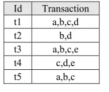
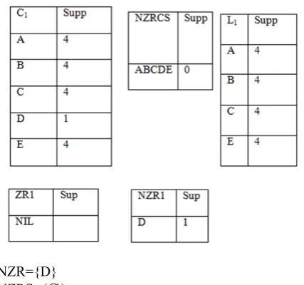
7.2 EXECUTION OF THE PROPOSED ALGORITHM IN DATASET D
Tid Itemset
1 A,B,D,E 2 A,C 3 A,B,C,E 4 B,C,E 5 A,B,C,E
Table 2. Dataset D Initialize:
C1= {A, B, C, D, E}, NZRCS= {ABCDE},
NZRS= ,K=1
Read the dataset to count the support of item sets in C1 and
NZRCS
NZR={D} NZRS={}
Second Pass:
NZRS={ABCE,ABDE} NZR={D,AD,BD,DE} Generate C3 using NZR2 U L2
Call NZRCS Generation procedure {
Since sup(ABCD)==0 so it is removed from NZRCS list and all 3 itemset of ABCD is added to NZRCS
Therefore
NZRCS={ACDE,ABCE,ABDE,BCDE,ABC,ABD,ACD,B CD}
Similarly for ACDE we get
NZRCS={ ABCE,ABDE,BCDE,ABC,ABD,ACD,BCD ,ADE,CDE}
For ABCE
Since sup(ABCE)is not equal to zero NZRS={ABCE,ABDE}
ABCEsub={ABC,ACE,BCE,ABE,AB,AC,AE,BC,BE,CE,A,
B,C,E}
Since no item in ABCEsub contain any item from NZR so
they are not added to NZRS and the three itemset is added to NZRCS.Thus we get
NZRCS={ ABDE,BCDE,ABC,ABD,ACD,BCD ,ADE,CDE,ACE,BCE,ABE}
For ABDE
Since Sup(ABDE) is not equal to zero NZRS={ABCE,ABDE}
ABDEsub={ABD,ADE,BDE,ABE,AB,AD,AE,BD,BE,DE,
A,B,D,E}
Now ABD,ADE,BDE,AD,BD,DE,D contain an item from NZR so they are also added to NZRS.Thus we get NZRS={ABCE,ABDE,ABD,ADE,BDE,AD,BD,DE,D} NZRCS={ BCDE,ABC,ABD,ACD,BCD
,ADE,CDE,ACE,BCE,ABE} For BCDE
Since sup(BCDE)==0 , so it is removed from NZRCS and all 3 itemset subset is added to NZRCS
Thus we get
NZRCS={ ABC,ABD,ACD,BCD ,ADE, CDE, ACE ,BCE , ABE, BDE}
Call Update NZRCS procedure using ZR2 }
Update NZRCS(NZRCS,ZR2) {
ZR2={CD} For CD in ZR2
And For all items in NZRCS
Since ACD,BCD and CDE contains CD as subset so they are removed from NZRCS
Thus we get
NZRCS={ ABC,ABD,ADE,ACE,BCE,ABE,BDE } }
Pass Three:
NZR={ D,AD,BD,DE ,ABC,ABD,ACE,ADE,BDE} Generate C4 using L3 U NZR3
Pass 4:
C5 will not be generated since L4 is NIL
And NZRCS generation procedure will not update the NZRS list
Thus we get
NZRS={ABCE,ABDE,ABD,ADE,BDE,AD,BD,DE,D,AB C}, which is the output of this algorithm.
7.3 Observation
It is observed that the proposed algorithm is able to find out the whole non zero rare item sets. Moreover it is able to prune out the zero rare item set. The main advantage of using this approach is that it reduces the number of candidate generation and minimizes the number of dataset scan. Moreover support count of some item sets can be find out without scanning the dataset by using Property 4 which states that “if X is a subset of Y and Sup(X) =Sup(Y) then any subset of Y which contain X will have same support as that of X and Y”.Also some non zero rare item set can be easily extracted without making a scan of the dataset by using Property1 and Property2.The proposed algorithm prune out zero item set by using property 3 which states that “if X is a zero item set then all its supersets are zero item set”.
Since we are maintaining two list NZRCS (top down direction) and Ck (bottom up direction) so information
gained in one direction can be used in the other direction and vice versa. For example if we have a zero item set in the Ck (bottom up direction) then all superset of it present
in NZRCS can be pruned out. Also if we have a non zero rare item set X in NZRCS(top down direction) and if it
contain a non zero rare item set Y from Ck list then any
subset of X that contains Y are also non zero rare item set. Thus we can have the following observation
If a nonzero rare item(X) in the bottom up direction is a subset of the longest nonzero rare item(Y) in the upward direction then any subset of the longest nonzero rare item(Y) which contains the X will also be nonzero rare items.
If a zero rare item(X) in the bottom up direction is a subset of the longest zero rare item(Y) in the upward direction then any subset of the longest zero rare item (Y) which contains X will also be zero rare items.
8.CONCLUSION AND FUTURE WORK
Mining rare patterns is a challenging endeavor because there are enormous number of such patterns that can be derived from a given data set. The key issues in mining infrequent patterns is to how to identify interesting infrequent patterns and how to effectively discover them in large data set.
In this paper we first highlight the importance of rare item set in some application. Then we proposes a methods for finding the non zero rare item set and finally we try to find interesting patterns from those item set. We have used the basic principle of Apriori Approach to find out the rare item set in a level wise bidirectional manner.
REFERENCES
[1] Adda, M., Wu, L., & Feng, Y. (2007). Rare item-set mining. Proceedings of the Sixth International Conference on Machine Learning and Applications (pp. 73–80). Washington, DC, USA: IEEE Computer Society.
[2] Agrawal, R., & Srikant, R. (1994). Fast algorithms for mining association rules in Large Databases. Proceedings of the 20th International Conference on Very Large Data Bases (pp. 487–499). San Francisco, CA, USA: Morgan Kaufmann Publishers Inc. [3] Agrawal, R., Imielinski, T., & Swami, A. (1993). Mining association
rules between sets of items in large databases. Proceedings of the 1993 ACM SIGMOD international conference on Management of data (pp. 207–216). Washington, D.C., United States: ACM. [4] Amor, N., Benferhat, S., & Elouedi, Z. (2004). Naive Bayes vs
decision trees in intrusion detection systems. ACM Symposium on Applied Computing (pp. 420–424). New York: ACM Press. [5] Barbara, D., Couto, J., Jajodia, S., & Wu, N. (2001). Adam: a testbed
for exploring the use of data mining in intrusion detection. Special Section on Data Mining for Intrusion Detection and Threat Analysis , 15–24.
[6] Chan, P., Mahoney, M., & Arshad, M. (2003). A machine learning approach to anomaly detection. Florida Institute of Technology. [7] Denning, D. (1987). An intrusion-detection model. IEEE
Transactions on Software Engineering, 222–232.
[8] DongJun, Z., Guojun, M., & Xindong, W. (2008). An Intrusion Detection Model Based on Mining Data Streams. Proceedings of The 2008 International Conference on Data Mining, DMIN (pp. 398–403). Las Vegas: CSREA Press.
[9] Gou, M., Norihiro, S., & Ryuichi, Y. (2002). A framework for dynamic evidence based medicine using data mining. Proceedings of the 15th IEEE Symposium on Computer-Based Medical Systems (p. 117). Maribor, Slovenia: IEEE.
[10] Haglin, D. J., & Manning, A. M. (2007). On minimal infrequent item-set mining. Proceedings of the 2007 International Conference on Data Mining, DMIN 2007 (pp. 141–147). Las Vegas, Nevada, USA: CSREA Press.
[12] Iwanuma, K., Takano, Y., & Nabeshima, H. (2004). On anti-monotone frequency measures for extracting sequential patterns from a single very-long data sequence. IEEE Conference on Cybernetics and Intelligent Systems, (pp. 213–217).
[13] Kumar, S., & Spafford, E. (1994). An application of pattern matching in intrusion detection. Technical Report 94–013, Department of Computer Sciences, Purdue University.
[14] Lane, T., & Brodley, C. (1997). An application of machine learning to anomaly detection. Proceedings of the 20th NIST-NCSC National Information Systems Security Conference, (pp. 366–380).
[15] Lee, W. (1998). Data mining approaches for intrusion detection. In Proceedings of the Seventh USENIX Security Symposium (pp. 6–6). San Antonio, Texas: USENIX Association Berkeley, CA, USA. [16] Mansfield, G., Ohta, K., Takei, Y., Kato, N., & Nemoto, Y. (2000).
Towards trapping wily intruders in the large. Computer Networks , 659–670.
[17] Pasquier, N., Bastide, Y., Taouil, R., & Lakhal, L. (1999). Efficient Mining Of Association Rules Using Closed Item-set Lattices. Information Systems, 25–46.
[18] Prati, R. C., Monard, M. C., André, C. P., & de Carvalho, L. F. (2004). A method for refining knowledge rules using exceptions, SADIO. Electronic Journal of Informatics and Operations Research , 53–65.
[19] Song, M., & Sanguthevar, R. (2006). A transaction mapping algorithm for frequent item-sets mining. IEEE Transactions on Knowledge and Data Engineering , 472–481.
[20] Srikant, R., & Agrawal, R. (1997). Mining Generalized Association Rules. Future Generation Computer Systems , 161–180.
[21] Szathmary, L., Maumus, S., Petronin, P., Toussaint, Y., & Napoli, A. (2006). Vers l'extraction de motifs rares. EGC: Extraction et Gestion de Connaissances, (pp. 499–510).
[22] Tan, K., Killourhy, K., & Maxion, R. (2002). Undermining an Anomaly-Based Intrusion Detection System Using Common Exploits. Recent Advances in Intrusion Detection , 54–73.
[23] Tiwari, A., Gupta, R., & Agrawal, D. (2010). A survey on frequent pattern mining: Current status and challenging issues. Inform. Technol , 1278–1293.
[24] Zaki, M. J., Parthasarathy, S., Ogihara, M., & Li, W. (1997). New algorithms for fast discovery of association rules. In Proceedings of the 3rd International Conference on Knowledge Discovery and Data Mining, (pp. 283–296).
[25] Zhan, J., & Leshan Teachers Coll., L. (2008). Intrusion Detection System Based on Data Mining. First International Workshop on Knowledge Discovery and Data Mining, 2008. WKDD 2008, (pp. 23–24). Adelaide, SA.
[26] Szathmary, L., Napoli, A., Valtchev, P.: Towards Rare Itemset Mining. In: Proceedings of the 19th IEEE International Conference on Tools with Artificial Intelligence (ICTAI ’07). Volume 1., Patras, Greece (Oct 2007) 305–312