Dynamic analysis of a spatial diffusion rumor propagation model with delay

R E S E A R C H

Open Access

Dynamic analysis of a spatial diffusion

rumor propagation model with delay

Chunru Li

_{and Zujun Ma}

*_{Correspondence:}

[email protected]

1_{Huaian College of Information}

Technology, Huaian, 223003, People’s Republic of China

2_{School of Transportation and}

Logistics, Southwest Jiaotong University, Chengdu, 610031, People’s Republic of China Full list of author information is available at the end of the article

Abstract

In this paper, we study the dynamics of a delayed reaction-diffusion rumor model with government control. By using the theory of partial functional differential equations, a Hopf bifurcation of the proposed system with delay as the bifurcation parameter is investigated. It reveals that the discrete time delay has a destabilizing effect in the rumor dynamics, and the phenomenon of Hopf bifurcation occurs as the delay increases through a certain threshold. Then by numerical simulations the impact of government control is explored. It is found that government control has strong effects on the dynamics of the model.

MSC: 34C23; 34D23

Keywords: rumor; spread; delay; diffusion

1 Introduction

Rumor is the kind of social phenomenon that a similar remark spreads on a large scale in a short time through chains of communication []. Compared with the way of rumor propagation by word of mouth in the old days, nowadays because of the appearance of the radio, television, newspapers, and mobile phone and so on, rumor appears and becomes widespread.

It is well known that the spreading of harmful rumors can deeply endanger a society. Most rumors induce panic psychology or economic loss in the accompanying unexpected events. Emergencies cause serious negative impacts on people’s life in several ways: not only the event itself might lead to financial loss or personal injuries, but also the rumor might lead to panic feelings and irrational behavior []. In order to reduce and avoid the dangers of the rumor propagation in online social networks, it is necessary to adequately understand the dynamic characteristics of rumor propagation. Rumor propagation is very similar to the diffusion of a virus, thus, most of the existing models of rumor propagation are derived from the models of infectious diseases [–]. The most popular model for information or rumor spreading, introduced by Daley and Kendall [, ], see also [, ], is conceptually similar to the SIR. This is a susceptible-infective-recovered model for epidemiology. Agents are divided into three classes: ignorants, spreaders, and stiflers,i.e., those who have lost interest in diffusing the information or rumor. Their role is exactly the same as the susceptible, infective, and recovered agents of the SIR model, respectively. Epi-demiological models have since been repeatedly used for describing information spread, such as topic flow in blog space, and word of mouth in product marketing.

The models mentioned above have concentrated only on the temporal dimension with-out diffusion. Recently, Wang et al.[] proposed a diffusive logistic (DL) model with spatial-temporal diffusion terms to study the information propagation process in online social networks. The authors described the spatial distance by using a new concept: friend-ship hops, and abstractly divided the information diffusion process in online social net-works into two separate processes: growth process and social process. In [], Wanget al.

further proposed a partial differential equation (PDE) based on a linear diffusive model to understand the information diffusion process over both temporal and spatial dimen-sions. Combined with the actual observations in the Digg data set, they proved the per-formance of the proposed linear diffusive model. To our knowledge, the study of a PDE rumor propagation model is still at the preliminary stage and there are many problems to be researched. Therefore, these spatial-temporal models will provide a new insight to research of the rumor propagation in online social networks.

It is worth noting that most works mentioned above on rumor propagation modeling assume that there is no time delay over rumor spreading. In fact, similarly to epidemic models [, ], as regards the rumor spreading process we should consider that there exists an incubation period before an influenced ignorant user has the ability to spread rumors. Consequently, delay needs to be considered.

In this paper, our objective is to propose a novel rumor propagation model with more realistic significance in theory and further analyze the dynamic characteristic of this model in mathematics.

The structure of this paper is arranged as follows. In Section , the modeling approach is described explicitly. In Section , we consider the existence of equilibrium points of system (), which is studied. In Section , we study the local stability and the existence of a Hopf bifurcation through the study of associated characteristic equations. In Section , we prove the global asymptotical stability of the interior equilibrium. In Section , some numerical simulations are given to support our theoretical predictions. Finally, this paper ends with a brief conclusion.

2 The model

This section describes a delayed spatial-temporal rumor propagation model. Our goal is to create a realistic model which can provide wide insight into predicting and controlling rumor prevalence in online social networks.

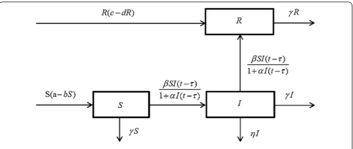
Generally, an online social network consists of many mobile Internet users. The geo-graphic position of a user is represented by the distancexfrom the rumor source []. At any time, a user is classified as either internal or external according to whether it is con-nected to the networks or not at that time. Based on the classical SIR epidemic model, in this work, the users in an online social network can be divided into three classes depend-ing on their different states: ignorants (those not aware of the rumor), spreaders (those who are spreading it), andRstiflers (those who know the rumor but have ceased commu-nicating it after meeting somebody already informed). For simplicity, we useI(t,x),S(t,x), andR(t,x) to represent the densities of ignorant users, spreading users, and stifle users with a distance ofxat timet, respectively. To model the propagation of rumor throughout online social networks, the following assumptions are imposed:

Figure 1 Node state transition relationship.

(ii) In online social networks, when an ignorant user is infected by spreading users, there is a spreading incubation period during which the infectious agents develop on networks, and it is only after that time that the infected user becomes himself infectious. Therefore, defining a delay for the spreading incubation period is more appropriate.

(iii) Usually, when a rumor spreading in online social networks the government will take effective actions to control and remove the spreading users.

Our assumption on the dynamical transfer of the nodes is depicted in Figure . As a result, our model can be represented as follows:

⎧ ⎪ ⎨ ⎪ ⎩ ∂S

∂t =dS+S(a–bS) –

βSI(t–τ) +αI(t–τ)–γS,

∂I

∂t =dI+

βSI(t–τ)

+αI(t–τ)–γI–ηI,

∂R

∂t =dR+R(c–dR) –γR+ηI,

()

whereSis for ignorants,Ifor spreaders, andRfor stiflers.a,b,c,d,d,d,γ,β,α, and

ηare all positive constants.di(i= , , ) are the diffusion coefficients of the users, be-ing used to describe the mobility.S(a–bS) andR(c–dR) represent ignorants and stiflers having logistic growth, respectively. _+βSI(t–_αI(t–τ_τ)₎ tends to a saturation level whenIgets large,

τ is a non-negative constant that represents the spreading incubation period, that is, it is only after the delay that the infected users become themselves infectious, and then they can spread rumors in online social networks.βI(t–τ) measures the infection force of the rumor and 

+αI(t–τ)measures the inhibition effect from the behavioral change of the

igno-rants individuals when their number increases or from the crowding effect of the infective individuals.γ is the death rate of nodes,ηis the government’s control power.

Here we assume the system has the following positive initial conditions and von Neu-mann boundary conditions:

∂S

∂φ = ∂I

∂φ = ∂R

∂φ = , t≥,x∈∂,

S(t,x) =ψ(t,x) > , I(t,x) =ψ(t,x), R(t,x) =ψ(t,x) > ,

(t,x)∈[–τ, ]×,

wheredenotes the Laplacian operator,is a bounded domain inRn_{with a smooth}

boundary∂andφ is the outside normal vector of∂. The boundary condition in () implies that there are no rumors across the boundary of . ψi(t,x) (i= , , ) are the

initial density functions. They are non-negative and Hölder continuous, and they satisfy

∂ψi/∂φ=  on (–∞, ]×∂.

3 Existence of equilibrium points

In this section, we will find all possible non-negative equilibria. Clearly, the system has four feasible non-negative equilibria, namely, () The trivial pointE(, , )T.

() The boundary equilibriumE(, ,c–_dγ)T, asc>γ, representing the state corresponding to the extinction of ignorants and spreaders.

() The boundary equilibriumE(a–_bγ, ,c–_dγ)T, asc>γ anda>γ, representing the

state corresponding to the extinction of the spreaders. () The interior equilibriumE∗(S∗,I∗,R∗)T_.

At the interior equilibrium point, we must have

⎧ ⎪ ⎨ ⎪ ⎩

(a–bS) –_+β_αI_I–γ = , βS

+αI –γ–η= , R(c–dR) –γI+ηI= .

()

Solving the second equation of (), we haveS=

β(γ +η)( +αI). SubstitutingSinto the first equation of (), we have

AI+AI+A= , ()

whereA=b(γ +η)α,A= αb(γ +η) +β–βα(a–γ),A=b(γ +η) –β(a–γ). For simplicity, we denote=A

– AA. The following results are obvious.

Lemma . For(),we have the following:

(a) If> andA< ,then()has a unique positive rootI∗=–A+

√

A .

(b) If= andA< ,then()has a unique positive rootI∗=–A

A.

(c) If> ,A> ,andA< ,then()has two positive rootsI∗=–A±

√

A .

As follows from Lemma ., system () will have at least one positive steady state

E∗(S∗,I∗,R∗), whereS∗=_β(γ+η)( +αI∗) andR∗=c–γ+

√

(c–γ)_+dηI∗

d .

4 Local stability and Hopf bifurcation

In this section, we will discuss the local stability and Hopf bifurcation of system () by analyzing the corresponding characteristic equations.

First, we make the following remarks:

α= I∗

 +αI∗, α= S∗

LetS˜=S–S∗,I˜=I–I∗,R˜=R–R∗, and substitute them in (). Dropping the bars for the simplicity of notation and retaining the linear terms inS,I, andRgive rise to

⎧ ⎪ ⎨ ⎪ ⎩ ∂S

∂t =dS+ (a– bS∗–βα–γ)S–βαI(t–τ),

∂I

∂t =dI+βαS+βαI(t–τ) – (γ +η)I,

∂R

∂t =dR+ηI+ (c– dR∗–γ)R.

()

Since the boundary condition is homogeneous von Neumann on the domainX, the ap-propriate eigenfunction of () is

(S,I,R) = (c,c,c)eλtcosnx, ()

wherenis the eigenvalue and the wave number. Substitution of this form in () yields

⎧ ⎪ ⎨ ⎪ ⎩

(λc+dnc)eλt_{cosnx= ((a– bS}∗_–βα

–γ)c–βαce–λτ)eλtcosnx,

(λc+dn_c)eλt_{cosnx= (βαc–βαce}–λτ_{– (γ +η)c)e}λt_cosnx,

(λc+dn_c)eλt_{cosnx= (ηc+ (c– dR}∗_–γ)c)eλt_cosnx.

()

Sinceeλt_{cosnx= , () is equivalent to the following set of linear algebraic equations:}

λ–a+ bS∗+βα+γ+dn βαe–λτ 

–βα λ–βαe–λτ+ (γ+η) +dn 

 –η λ+dn–c+ dR∗+γ

c

c

c

= .

()

Nontrivial solutions to () exist if and only if

det

λ–a+ bS∗+βα+γ+dn βαe–λτ 

–βα λ–βαe–λτ+ (γ+η) +dn 

 –η λ+dn–c+ dR∗+γ

= .

()

Equation () is equivalent to the following equation:

(λ+Cn)λ+ (An+Bn)λ+AnBn+ (βα–An–λ)αβe–λτ = , n= , , , . . . , ()

where

An= –a+ bS∗+βα+γ +dn, Bn=dn+γ +η, Cn=dn+ dR–c+γ.

()

We make the following assumptions:

(H) a>γ;

(H) c<γ;

Whenn= , the characteristic equation () about the equilibrium pointE(, , ) takes the form

(λ+γ –c)λ+ (γ+η–a)λ+ (γ–a)(γ+η) = . () For the equilibrium pointE(, ,c–_dγ)T, asn= , () reduces to

(λ+c–γ)λ+ (γ+η–a)λ+ (γ–a)(γ+η) = . () For the boundary equilibriumE(a–_bγ, ,c–_dγ)T_{, asn= , () becomes}

(λ+c–γ)

λ+

 –β

b

a+η+βγ

b

λ–β(a–γ)



b

= . ()

By a simple calculation, we have the following: () and () both have a positive root if (H) holds, () has at least a positive one positive root, asτ= . Therefore, we obtain the

following results.

Theorem . If(H)holds,then the boundary equilibrium Eand E are both unstable. Asτ= ,Eis unstable.

In the following part, we analyze the stability and Hopf bifurcation about the interior equilibriumE∗(S∗,I∗,R∗)T_.

Asτ= , () is equivalent to the following cubic equation: (λ+Cn)

λ+ (An+Bn–αβ)λ+AnBn+βαα–Anαβ = , n= , , , . . . . ()

It is obvious thatλ=  is not a root of ()∀n∈N{, , , . . .}, as (H) holds. Lemma . If(H)and(H)hold,thenλ= is not a root of()for∀n≥and the interior equilibrium E∗of system()withτ = is locally asymptotically stable.

Proof Clearly, from () we have

λ=c–γ– dR∗–dn,

λ+λ= –An–Bn+αβ

=αβ–a– bS∗–βα– γ–dn–dn–η,

λλ=βαα–Anαβ+AnBn.

()

If (H) and (H) hold, thenλ< ,λandλhave negative real parts. So, system () with

τ =  is locally asymptotically stable.

For further discussion, we denote

A= –a+ bS∗+βα+γ, B=γ+η,

(H) –a+ bS∗+βα+γ > ,

(H) AB+Aβα–βαα< ,

(H) dA–βαα> .

Now we discuss the effect of the delayτ on the stability of the trivial solution of (). Assume thatiωis a root of (). Thenωshould satisfy the following equation for some

n≥:

–ω+i(An+Bn–βα)ω+AnBn

+βαα–Anβα–iβωα

cos(ωτ) –isin(ωτ)= , ()

which implies that

ω_{–AnBn= –βωα}

sin(ωτ) + (βαα–Anβα)cos(ωτ),

(An+Bn)ω= (β_α

α–Anβα)sin(ωτ) +βωαcos(ωτ).

()

From (), adding the squared terms for both equations yields

ω+A_n+B_n–βαω+A_nB_n–βαα–Anβα



= . ()

Letz=ω, () becomes

z+A_n+B_n–βαz+A_nB_n–βαα–Anβα



= , ()

where

A_n+B_n–βα=d_n+d_n+d–a+ bS∗+βα+γ

+ d(γ +η)n

+–a+ bS∗+βα+γ



+ (γ+η),

A_nB_n–βαα–Anβα



=AnBn+βαα–Anβα

AnBn–βαα+Anβα

.

()

Theorem . If(H)-(H)hold,then all roots of()have negative real parts for allτ≥. Furthermore,the interior equilibrium E∗of system()is asymptotically stable for allτ≥.

Proof From hypothesis (H), we know thatAnBn+βαα–Anβα> . We have

AnBn–βαα+Anβα=ddn+ (dB+dA)n+AB+Aβα–βαα.

If (H) holds,AnBn–βαα+Anβα> . These results imply that () has no positive

roots, and hence the characteristic equation () has no purely imaginary roots. Combine with Lemma ., all roots of () have negative real parts asτ ≥. This completes the

proof.

Remark  In Section , we will prove that when (H)-(H) hold, then the interior

Lemma . If(H)and(H)hold,then()has a unique positive root,as n= .

Proof By hypothesis (H), we know thatAB+βαα–Aβα> . We have AB–βαα+Aβα=AB+Aβα–βαα.

If (H) holds,AB–βαα+Aβα< . Therefore, according to Descartes’ rule of

signs [], () has a unique positive root.

According to Lemma ., () has a unique positive root, denoted byz, and thus ()

has a unique positive rootω=√z. By (), we have

Then we obtain

Substitutingτ_j into the above equation, we obtain

From the above analysis, we have the following theorem.

Theorem . Based on Lemmas.-.,the following statements are true: (i) Whenτ∈[,τ),the positive steady state of()is locally asymptotically stable.

(ii) A Hopf bifurcation occurs atτ=τ.That is,system()has a branch of periodic solutions bifurcating from the zero solution nearτ=τ.

5 Global stability

In this section, we prove that when (H)-(H) hold, the interior equilibrium is indeed

glob-ally asymptoticglob-ally stable. To achieve this, we utilize the upper-lower solution method in [, ].

Proof From the first equation of system (), we have

∂S

∂t =dS+S(a–bS) –

βSI(t–τ)  +αI(t–τ)–γS

≤dS+S(a–bS) –γS, ()

then from the comparison principle of parabolic equations and Lemma ., for an arbitrary

ε> , there existst(> ) such that for anyt>t,

wherec¯ =a–_bγ +ε. This implies

lim sup

t→+∞ maxx∈ ¯

S(·,t)≤a–γ

b .

Therefore, from the second equation of system () and (), we have

∂I

∂t =dI+

βSI(t–τ)

 +αI(t–τ)–γI–ηI

≤dI+

β(a–_bγ +ε)I(t–τ)

 +αI(t–τ) –γI–ηI, ()

fort>t+τ. Hence there existst>tsuch that, for anyt>t,

v(x,t)≤ ¯c, ()

wherec¯=β(a–γα+bb(ηε)–b(+γ)η+γ)+ε. Again this implies

lim sup

t→+∞ maxx∈ ¯

I(·,t)≤β(a–γ) –b(η+γ)

αb(η+γ) .

From the third equation of system () and (), we obtain

∂R

∂t =dR+R(c–dR) –γR+ηI

≤dR+R(c–dR) –γR+η¯c, ()

fort>t. Hence there existst>tsuch that, for anyt>t,

R(x,t)≤ ¯c, ()

wherec¯=

c–γ+√(c–γ)_+dη¯c 

d +ε. Again this implies

lim sup

t→+∞ maxx∈ ¯

R(·,t)≤

c–γ +

(c–γ)_{+ dη}β(a–γ)–b(η+γ)

αb(η+γ)

d .

On the other hand, from the first equation of system () and (), we have

∂S

∂t =dS+S(a–bS) –

βSI(t–τ)  +αI(t–τ)–γS

≥dS+S

a–bS– βm¯  +αm¯

–γ

, ()

fort>t. Since (H)-(H) hold, for small enoughε>  such that a–γ

b( +αc¯) +βc¯

there existst>tsuch that, for anyt>t,

S(x,t)≥c_, ()

where

c_= a–γ

b( +α¯c) +βc¯ –ε. ()

Then we apply the lower bound ofSto the third equation of system (), and we have

∂I

∂t =dI+

βSI(t–τ)

 +αI(t–τ)–γI–ηI

≥dI+ βcI(t–τ)

 +αI(t–τ)–γI–ηI, ()

fort>t. Then there existst>tsuch that, for anyt>t,

I(x,t)≥c_, ()

where

c_=βc–γ–η

α(γ+η) +ε. () Finally, we apply the lower bound ofIto the second equation of system (), and we have

∂R

∂t =dR+R(c–dR) –γR+ηI

≥dR+R(c–dR) –γR+ηc_, ()

fort>t. Then there existst>tsuch that for anyt>t,

R(x,t)≥c_, ()

where

c_=c–γ +

(c–γ)_{+ dηc} 

d +ε. ()

From (), (), and (), we can easily obtain

lim inf

t→+∞ maxx∈ ¯

S(·,t)≥c_, lim inf

t→+∞ maxx∈ ¯

I(·,t)≥c_, lim inf

t→+∞ maxx∈ ¯

R(·,t)≥c_. ()

It is easily found that

andc_,¯c,c_,c¯ ,c_,c¯ satisfy lower solutions of system () as in the definition in [, ]. It is easy to show that there is a positive constantKsuch that the following Lipschitz condition holds:

Therefore

In this section, we present numerical simulations of some examples to illustrate our the-oretical results.

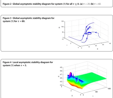
6.1 Stability of the positive steady state for all

τ

Let the parameters of system () bed= .,d= ,d= ,a= .,b= .,β= .,γ = .,

c= .,d= .,α= ., andη= .. Calculation reveals that the interior equilibrium of system () is (., ., .)T_{. Obviously, the conditions (H}

)-(H) hold.

Ac-cording to Theorem ., system () has global asymptotic stability at the positive steady state for allτ≥, as shown in Figure  and Figure . This means that with these parameter values the number of spreaders will be constant for any delayτ> .

6.2 Stability and Hopf bifurcation of system (1)

Let d = ., d = , d = , a= ., b= ., β = ., γ = ., c= ., d= .,

α = ., andη= .. Calculation reveals that the interior equilibrium of system () is (., ., .)T_{and the critical value isτ}

= .. Obviously, the parameters

satisfy (H)-(H) and (H)-(H). According to Theorem ., system () has local

(a) (b)

Figure 2 Global asymptotic stability diagram for system (1) for allτ≥0. (a)τ= 20;(b)τ= 60.

Figure 3 Global asymptotic stability diagram for system (1) forτ= 80.

Figure 4 Local asymptotic stability diagram for system (1) whenτ= 3.

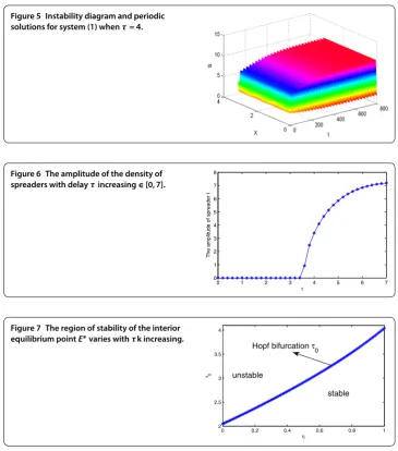
as observed in Figure  and Figure . As Figure  has shown, whenτ=  the spatially ho-mogeneous periodic solutions emerge from the interior equilibriumE∗, which implies the rumor explosively spreads in a short period and may destroy network stability and block regular communications in online social networks, or even cause panic in the real society.

Remark  Keep the parameters d= .,d= ,d= , a= .,b= .,β= .,γ = .,c= .,d= .,α= ., andη= .. In this part, we discuss the effect of delay

Figure 5 Instability diagram and periodic solutions for system (1) whenτ= 4.

Figure 6 The amplitude of the density of spreaders with delayτincreasing∈[0, 7].

Figure 7 The region of stability of the interior equilibrium pointE∗varies withτk increasing.

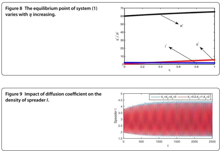
6.3 Effect of the government adjustment power

Taking the parameters the same as in Section ., butηvarying in [, ], the corresponding locations of the equilibrium points are shown in Figure  and the stable range of system () is shown in Figure . Numerical evidence shows that with the increase of the adjustment power η, the adjustment power makes the population of the spreaders reduce and the population of the ignorants and stiflers increase. Figure  shows that with the growth of the adjustment powerηthe stability range is increasing. This is to say, if the government applies TV (the most popular and most believed medium in China)e.g.to announce the truth, the population of the spreaders will be reduced immediately.

6.4 The effect of the diffusion

To observe the impact of diffusion coefficient on the spreaderI, we leta= .,b= .,

β= .,γ = .,c= .,d= .,α= ., andη= ., and assign , ,  and ., ,  tod,d,d, respectively. Obviously, condition (H)-(H) and (H)-(H) hold. According

Figure 8 The equilibrium point of system (1) varies withηincreasing.

Figure 9 Impact of diffusion coefficient on the density of spreaderI.

homogeneous periodic solutions emerge from the interior equilibriumE∗, as shown in Figure . From it, we notice that the rumor propagation in online social networks goes into periodic oscillation. In addition, from Figure  we notice that whend= .,d= ,

d=  the amplitude of the density of spreaderIdecreases. In fact, by a simple calculation,

it is easy to see when d =d=d=  that the oscillation of the rumor propagation is . and the oscillation decreases to . whend= .,d= ,d= , which means the mobility of nodes decreases the degree of oscillation of the rumor propagation. The above observations show that the diffusion we incorporated into the system can affect the amplitude of system ().

7 Conclusion

In this paper, we introduced delay and diffusion into a rumor model. Through the theo-retical analysis and numerical simulation we found that government adjustment powerη

can affect the system’s stability. These can be found in Section ..

By using PDE stability theory, we take the delayτ as the bifurcation parameter to study the Hopf bifurcation of system (). Theoretical analysis and numerical simulations show that the discrete delay is responsible for the stability switch of the model and a Hopf bifur-cation occurs as the delays increase through a certain threshold (see Section .). When (H)-(H) hold, the interior equilibrium is globally asymptotically stable.

In summary, our study contributes to rumor management in an emergent event by offer-ing an interplay model between rumor spreadoffer-ing and government adjustment. Accordoffer-ing to the transmission of the rumor, the government should apply TV (the most popular and most believed medium in China) to announce the truth, and the population of the spread-ers will be reduced immediately.

Competing interests

Authors’ contributions

CL conceived of the study, drafted the manuscript, participated in the sequence alignment, and performed the numerical analysis. ZM helped to revise the manuscript. All authors read and approved the final manuscript.

Author details

1_{Huaian College of Information Technology, Huaian, 223003, People’s Republic of China.}2_{School of Transportation and}

Logistics, Southwest Jiaotong University, Chengdu, 610031, People’s Republic of China.3_{School of Economics and}

Management, Southwest Jiaotong University, Chengdu, 610031, People’s Republic of China.

Acknowledgements

The work is supported by National Natural Science Foundation of China under Grant 90924012. The authors also gratefully acknowledge the helpful comments and suggestions of the reviewers, which have improved the presentation.

Received: 18 May 2015 Accepted: 30 September 2015 References

1. Kawachi, K, Seki, M, Yoshida, H, Otake, Y, Warashina, K, Ueda, H: A rumor transmission model with various contact interactions. J. Theor. Biol.253(1), 55-60 (2008)

2. Zhao, L, Wang, Q, Cheng, J, Zhang, D, Ma, T, Chen, Y, Wang, J: The impact of authorities media and rumor dissemination on the evolution of emergency. Phys. A, Stat. Mech. Appl.391(15), 3978-3987 (2012)

3. Lin, T, Fan, C, Liu, C, Zhao, J, et al.: Optimal control of a rumor propagation model with latent period in emergency event. Adv. Differ. Equ.2015, 1 (2015)

4. Huo, L, Huang, P, Guo, C-x: Analyzing the dynamics of a rumor transmission model with incubation. Discrete Dyn. Nat. Soc.2012, 328151 (2012)

5. Huo, L, Huang, P: Study on rumor propagation models based on dynamical system theory. Math. Pract. Theory 43(16), 1-8 (2013)

6. Huo, L-a, Huang, P, Fang, X: An interplay model for authorities actions and rumor spreading in emergency event. Phys. A, Stat. Mech. Appl.390(20), 3267-3274 (2011)

7. Zhao, L, Wang, Q, Cheng, J, Chen, Y, Wang, J, Huang, W: Rumor spreading model with consideration of forgetting mechanism: a case of online blogging LiveJournal. Phys. A, Stat. Mech. Appl.390(13), 2619-2625 (2011) 8. Zhao, L, Wang, J, Chen, Y, Wang, Q, Cheng, J, Cui, H: SIHR rumor spreading model in social networks. Phys. A, Stat.

Mech. Appl.391(7), 2444-2453 (2012)

9. Zhao, L, Xie, W, Gao, HO, Qiu, X, Wang, X, Zhang, S: A rumor spreading model with variable forgetting rate. Phys. A, Stat. Mech. Appl.392(23), 6146-6154 (2013)

10. Zhou, J, Liu, Z, Li, B: Influence of network structure on rumor propagation. Phys. Lett. A368(6), 458-463 (2007) 11. Xiong, F, Liu, Y, Zhang, Z-j, Zhu, J, Zhang, Y: An information diffusion model based on retweeting mechanism for

online social media. Phys. Lett. A376(30), 2103-2108 (2012)

12. Daley, DJ, Gani, J: Epidemic Modelling. Cambridge University Press, Cambridge (2000)

13. Daley, DJ, Kendall, DG: Efficiency and reliability of epidemic data dissemination in complex networks. IMA J. Appl. Math.1, 42-55 (1965)

14. Moreno, Y, Nekovee, M, Pacheco, AF: Dynamics of rumor spreading in complex networks. Phys. Rev. E69(6), 066130 (2004)

15. Moreno, Y, Nekovee, M, Vespignani, A: Efficiency and reliability of epidemic data dissemination in complex networks. Phys. Rev. E69(5), 055101 (2004)

16. Wang, F, Wang, H, Xu, K: Diffusive logistic model towards predicting information diffusion in online social networks. In: 2012 IEEE 32nd International Conference on Distributed Computing Systems Workshops (ICDCSW), pp. 133-139 (2012)

17. Wang, F, Wang, H, Xu, K, Wu, J, Jia, X: Characterizing information diffusion in online social networks with linear diffusive model. In: 2013 IEEE 33rd International Conference on Distributed Computing Systems (ICDCS), pp. 307-316 (2013)

18. Xu, R, Ma, Z: Global stability of a SIR epidemic model with nonlinear incidence rate and time delay. Nonlinear Anal., Real World Appl.10(5), 3175-3189 (2009)

19. Yang, J, Liang, S, Zhang, Y: Travelling waves of a delayed SIR epidemic model with nonlinear incidence rate and spatial diffusion. PLoS ONE6(6), 1786-1788 (2011)

20. Wang, F, Wang, H, Xu, K: Diffusive logistic model towards predicting information diffusion in online social networks. In: ICDCS’12 Workshops, pp. 133-139 (2011)

21. Descartes, R: The Philosophical Writings of Descartes, vol. 2. Cambridge University Press, Cambridge (1985) 22. Pao, C-V: Dynamics of nonlinear parabolic systems with time delays. J. Math. Anal. Appl.198(3), 751-779 (1996) 23. Pao, C-V: Convergence of solutions of reaction-diffusion systems with time delays. Nonlinear Anal., Theory Methods

Appl.48(3), 349-362 (2002)