R E S E A R C H
Open Access
Mean-square numerical approximations
to random periodic solutions of stochastic
differential equations
Qingyi Zhan
**Correspondence: [email protected] College of Computer and Information Science, Fujian Agriculture and Forestry University, Fuzhou, 350002, P.R. China Institute of Computational Mathematics and
Scientific/Engineering Computing, Chinese Academy of Sciences, Beijing, 100190, P.R. China
Abstract
This paper is devoted to the possibility of mean-square numerical approximations to random periodic solutions of dissipative stochastic differential equations. The existence and expression of random periodic solutions are established. We also prove that the random periodic solutions are mean-square uniformly asymptotically stable, which ensures the numerical approximations are feasible. The convergence of the numerical approximations by the random Romberg algorithm is also proved to be mean-square. A numerical example is presented to show the effectiveness of the proposed method.
Keywords: stochastic differential equation; random periodic solutions; random Romberg algorithm; pullback; forward infinite horizon stochastic integral equations
1 Introduction
Stochastic differential equations (SDEs) have an important position in theory and appli-cation, for more details we refer the reader to [] and []. In recent years, there has an increasing interest in random periodic solutions of SDEs. Random periodic solutions de-scribe many physical phenomena and play an important role in aeronautics, electronics, biology, and so on [, ]. The existence of random periodic solutions was established by Fenget al.[]. However, random periodic solutions have not been explicitly constructed as yet. Therefore, numerical approximations to random periodic solutions are an important method for studying their dynamic behavior. There are, however, few numerical studies in this field. The main difficulties lie in determining the initial value at the starting time and simulating improper integrals more efficiently. Therefore, we are concerned with the pos-sibility of mean-square numerical approximation and numerical analysis of convergence in this paper.
There are two main motivations for this work. It is well known that, in the deterministic case, some researchers have obtained extensive results, including numerical approxima-tions to periodic solution. We refer the reader to [] and [] and the references therein. However, few studies have been done in the random case. Yevik and Zhao [] treated the numerical stationary solutions of SDEs. Liuet al.[] investigated square-mean almost periodic solutions for a class of stochastic integro-differential equations. To the best of our knowledge, no investigations of mean-square numerical approximations to random
periodic solutions of SDEs exist in the literature. Numerical approximation is still an in-teresting method for studying random periodicity in random dynamical systems.
Because there exist errors in the initial value at the starting time, and the random peri-odic solutions are sensitive to the initial value, we can only deal with SDEs whose random periodic solutions are mean-square uniformly asymptotically stable. The main results we obtain are the numerical approximations to random periodic solutions of dissipative SDEs, and the proof of mean-square convergence. This shows that mean-square numerical ap-proximations to random periodic solutions are in fact close to the exact solutions and the iterative error can be controlled in the range of the presupposed error tolerance.
This paper is organized as follows. Section deals with some preliminaries intended to clarify the presentation of concepts and norms used later. In Section we present theoret-ical results on random periodic solutions of dissipative SDEs. This is the main conclusion of the article, which contains the existence and stability of random periodic solutions, the numerical implementation method and the mean-square convergence theorem. Section is devoted to numerical experiments, which demonstrate that these algorithms can be ap-plied to simulate random periodic solutions of dissipative SDEs. Finally, Section gives some brief conclusions.
2 Preliminaries
LetW(t),t∈Rbe ank-dimensional Brownian motion, and (,F,P) be the filtered Wiener space. HereFt
s:=σ(Wu–Wv,s≤v≤u≤t), andFt:=
s≤tFst, wheres∈Ris any given time []. We consider a class of Itô SDE of the form
dXt= –AXtdt+f(t,Xt)dt+g(t)dWt, X(s) =x∈Rd, ()
whereXt:→Rd,f :R×Rd→Rd,g:R→Rd×k,Ais a class ofd×dhyperbolic matrix whose all eigenvalues are positive, and we defineTt=e–At to be a hyperbolic linear flow induced by –A.
We define
θ: (–∞, +∞)×→, θtω(s) =ω(t+s) –ω(t) ()
and:={(s,t)∈R,s≤t}. By the conclusions in [], SDE () generates a stochastic flow ϕ:×Rd×→Rdwhen the solution of SDE () exists uniquely, which is usually written asϕ(s,t,x,ω) :=ϕ(s,t,ω)xon the metric dynamical systems (,F,P,θt). The stochastic flowϕis given by
ϕ(s,t,ω)x=x+
t
s
–Aϕ(s,r,ω)x+fr,ϕ(s,r,ω)xdr+
t
s
g(r)dWr, t≥s. ()
Throughout the rest of this paper, we make the following notations.
LetL(,P) be the space of all bounded square-integrable random variablesx:→Rd. For any random vectorx= (x,x, . . . ,xd)∈Rd, the norm ofxis defined in the form of
x=
x(ω)
+x(ω)
+· · ·+xd(ω)
dP
For any stochastic processx(t,ω)∈Rd, the norm ofx(t,ω) is defined as follows:
x(t,ω)=sup t∈R
xt(ω)<∞.
We define the norm of random matrices as follows:
GL(,P)=
E|G| , ()
whereGis a random matrix and| · |is the operator norm.
For simplicity in notations, the norms · and · L(,P)are usually written as · . The following hypotheses are made for the theoretical analysis.
Hypothesis .
(i) There exists a constantK∗> such thatx ≤K∗.
(ii) The mappingf :R×Rd→Rdis continuous,and there exist positive constantsJ andKsuch thatf(t, )is globally bounded with|f(t, )| ≤Jand for any X,X∈Rd,the following inequality holds:
f(t,X) –f(t,X)≤K|X–X|. ()
(iii) The mappingg:R→Rdis continuous,and there exists a positive constantJsuch thatg(t)is globally bounded with|g(t)| ≤J.
3 Theoretical results
3.1 Existence of random periodic solutions
The following result guarantees the existence of random periodic solutions for dissipative SDEs, and is a direct consequence of Theorem .. in [].
Lemma . For any–∞<s≤t< +∞,x,xˆ ∈B,if the following conditions hold:
(i) ϕ(s,t,ω)·:B→Bis a.s.continuous; (ii) ϕ(s+τ,t+τ,ω)x=ϕ(s,t,θτω)x;
(iii) there exist constantsc∈(, )andM> such that
ϕ(s,t,ω)x–ϕ(s,t,ω)xˆ ≤ct–sx–xˆ andϕ(s,t,ω)x ≤M,whereMmay depend on(t–s),
then there exists a unique random τ-periodic solution Y(t,ω) of ϕ. Moreover, ϕ(t – mτ,t,θ–mτω)x→Y(t,ω)∈Lp(,B)as m→+∞,where B⊂Rd and m is a positive
in-teger.
Lemma . Suppose that A is a class of hyperbolic d×d matrix,the eigenvalues of A are denoted by{λj,j= , , . . . ,d}and satisfy <λ≤λ≤ · · · ≤λd.Then the function e–At tends to zero as t→+∞,that is,
lim t→+∞e
–At= .
lim t→+∞e
–At= lim
t→+∞e –λt= ,
whereλ> .
So it is valid for the one-dimensional case.
Now we consider the case d> . The matrix exponential of Ais diagonalizableeA= QeDQ–, whereAis invertible andDis diagonal with eigenvalues ofAas its spectrum []. Then we get
e–At=Qe–DtQ–
and
e–Dt=
⎛ ⎜ ⎜ ⎜ ⎜ ⎝
e–λt · · · e–λt · · ·
..
. ... ... ... ... · · · e–λdt
⎞ ⎟ ⎟ ⎟ ⎟ ⎠.
It follows from the result of the one-dimensional case that it is also valid for the d-dimensional case. This completes the proof.
From the conclusions of Lemmas . and ., we obtain the following theorem.
Theorem . Assume that there exists a constantτ> such that for any t∈R and any X∈Rd,the following equalities hold:
f(t,X) =f(t+τ,X), g(t) =g(t+τ). ()
Suppose that A satisfies Lemma..Moreover,suppose that SDE()satisfies Hypothesis. and the global Lipschitz constant of f be K∈[,
√
λd).
If SDE()has a unique random periodic solution Y(t,ω) : (–∞, +∞)×→Rd,that is,
ϕ(t,t+τ,ω)Y(t,ω) =Y(t+τ,ω) =Y(t,θτω), for all t∈R a.s. ()
then Y(t,ω)is a solution of the forward infinite horizon integral equation
Y(t,ω) =
t
–∞Tt–rf
r,Y(r,ω)dr+ (ω)
t
–∞Tt–rg(r)dWr. ()
Proof In order to utilize Lemma . to this problem, we only need to check that the con-ditions of this theorem satisfy its three hypotheses.
First and foremost, by the assumptions of SDE (), the hypothesis (i) obviously holds. Secondly, utilizing () and Duhamel’s formula, we obtain
ϕ(s,t,ω)x
=e–A(t–s)x+
t
s
e–A(t–r)fr,ϕ(s,r,ω)xdr+ (ω)
t
s
Using () and (), we have
By the uniqueness of the solution, we obtain
¯
This completes the check of the second hypothesis.
By the condition () we have
By the Gronwall inequality, there exists a numberMsuch that
ϕ(s,t,ω)x–ϕ(s,t,ω)xˆ ≤M,
Using the Cauchy-Schwarz inequality and the Itô isometry we have
Eϕ(s,t,ω)x≤e–A(t–s)E|x|+
From the global Lipschitz condition of the functionf it follows that for anyX∈Rd, the linear growth condition also holds:
f(t,X)≤K|X|+J. ()
From the globally boundedness of the functiongand the boundedness of the initial value in Hypothesis ., we obtain
Eϕ(s,t,ω)x≤KK∗+ KJ(t–s) + KJ(t–s) + KK·
t
s
Eϕ(s,r,ω)xdr.
By the Gronwall inequality, there exists a numberMsuch that
where
M=
KK∗+ KJ(t–s) +KJ(t–s) ·expKK(t–s).
HereMsatisfies the assumption that it may depend ont–s. This completes the check of the third hypothesis.
Moreover, the pullback method only works for dissipative systems, that is, the systems are contractive. The pullback of SDE () is
dX(t–mτ,t,θ–mτω,x)
Therefore, the exact solution of SDE () at the timethas the form
ϕ(t–mτ,t,θ–mτω)x=e–Amτx+
It follows from Lemma . and the periodic property off andgthat
lim
Therefore, the conclusion follows from Lemma . and Theorem .. in []. The proof is
finished.
3.2 Stability
Definition . (i) The random periodic solutionY(t,ω) of SDE () is said to be
mean-square asymptotically stable if for any given> , every other random periodic solution
ˆ
Y(t,ω) of SDE () satisfies
lim
t→+∞Y(t,ω) –Y(t,ˆ ω)=
for any boundedFs-measurable bounded initial valuesxandx, respectively, whereˆ x–
ˆ
x<, wheres=t–mτ.
(ii) The random periodic solutionY(t,ω) of SDE () is said to be mean-square uniformly stable if for any given> and every other random periodic solutionY(t,ˆ ω) of SDE (), there existsδ=δ() such thatx–xˆ ≤δimplies the inequalityY(t,ω) –Y(t,ˆ ω)< holds for anyt≥s, wheres=t–mτ.
(iii) The random periodic solutionY(t,ω) of SDE () is said to be mean-square uniformly asymptotically stable if it is mean-square uniformly stable and mean-square asymptoti-cally stable.
Theorem . Assume that for any initial values xandxˆ ∈L(,P),the coefficients of SDE()satisfy Theorem.,then the random periodic solution Y(t,ω)of SDE()is mean-square uniformly asymptotically stable.
Proof First and foremost, letϕ(t–mτ,t,θ–mτω)xˆ be another solution of SDE () and>
be an arbitrary constant. Ifx–xˆ ≤, it follows from () and the method which is used to estimate () that
Eϕ(t–mτ,t,θ–mτω)x–ϕ(t–mτ,t,θ–mτω)xˆ
≤KE|x–xˆ |+ KK
t
t–mτ
Eϕ(r,t,θ–mτω)x–ϕ(r,t,θ–mτω)xˆ
dr,
where
K=e–Amτ and K=
t
t–mτ
e–A(t–r)dr.
By the Gronwall inequality, there exists a numberMsuch that
ϕ(t–mτ,t,θ–mτω)x–ϕ(t–mτ,t,θ–mτω)xˆ ≤M,
where
M=x–xˆ
K·expKK mτ
.
Therefore, by the fact thatM→ asm→+∞, we obtain
lim
Fatou’s lemma implies that
EY(t,ω) –Yˆ(t,ω)=E
lim
m→+∞ϕ(t–mτ,t,θ–mτω)x–ϕ(t–mτ,t,θ–mτω)xˆ
≤ lim
m→+∞Eϕ(t–mτ,t,θ–mτω)x–ϕ(t–mτ,t,θ–mτω)xˆ
.
Then we have
lim
t→+∞Y(t,ω) –Y(t,ˆ ω)= .
Then by Definition .(i), it is mean-square asymptotically stable.
Secondly, let V(s,t,ω)x¯ =Y(t,ω) –Yˆ(t,ω), where x¯ = (x,x). It is the fact thatˆ V(s,t,ω)x¯ is also a random periodic solution of SDE (). Without loss of generality, we only consider the cases≥. The proof of other case is similar, that is, by the transforma-tions˘=s+mτ, we can change the case ofs≤ to the case of˘s≥, wheremis a positive integer. Letx¯be the initial value at the starting times= . From the above result, that is, the mean-square asymptotic stability, it follows that for any given> , there exists δ=δ() > such thatx–xˆ ≤δimplies the inequalityV(,t,ω)x¯< holds for t≥.
For the first cases∈[,τ], by the fact thatV(s,t,ω)x¯is continuous with respect to (s,x¯) and uniformly continuous with respect tosfors∈[,τ], there existsδ=δ() > such that
x–xˆ ≤δimplies the inequalityV(s, ,ω)x¯<δholds fors∈[,τ].
Putx¯=V(s, ,ω)x, and we obtain¯ V(s,t,ω)x¯ =V(,t,θsω)x¯for anyt≥. Therefore ifx–xˆ ≤δands∈[,τ], the inequalityV(s,t,ω)x¯<holds for anyt≥s, that is,
Y(t,ω) –Yˆ(t,ω)<.
For the second case s> , there exists a positive integer m such that s ∈[mτ, (m+ )τ]. It follows from the random periodicity thatV(s–mτ,t–mτ,θ–mτω)x¯is also the random periodic solution of SDE () and
V(s,t,ω)x¯=V
s–mτ,t–mτ,θ–mτω
¯
x.
Thenx–xˆ ≤δimplies the inequalityY(t,ω) –Yˆ(t,ω)<holds for anys≥ and t≥s.
Therefore it follows from Definition .(ii) that it is mean-square uniformly asymptoti-cally stable. The conclusion follows from Definition .(iii). This completes the proof.
3.3 Numerical implementation method of random periodic solutions
that the numerical solution to initial problem is the numerical solution to the random periodic solution.
Therefore, a numerical implementation method is as follows. We obtain from (),
Y(,ω) =
which can be viewed as the initial value at the timet= of random periodic solutions of SDE (). The finite time interval [,t] is divided intoN subintervals with the length t:= t
then the improper integral () can be approximated by the Itô integralY¯(,ω), where
¯
Therefore the improper integral () in the finite time interval [,t] can be approximated by the Itô integral ()
˜
By means of reselecting the corresponding starting time ands, we can simulate a ran-dom periodic solution in an arbitrary finite time interval with any given presupposed error tolerance.
In order to improve the accuracy of the integral, the random Romberg algorithm is ap-plied to () andY(,¯ ω). The method applied to () in detail is shown as follows.
then we see that the iterative relation
˜
Wtn=W(nt) –W(), Wtn=
From the induction principle, it implies that
Rj=
Utilizing the extrapolation method, we obtain the element
Rjk= k–R
j,k––Rj–,k–
k–– , k= , . . . ,j. ()
For any presupposed error toleranceε∈[,δ], if the inequality holds
Rj,j––Rjj ≤ε,
the computation is ended andRjjis viewed as the approximation of (). That is,
˜
Yn(t,ω) =Rjj.
The method applied toY(,¯ ω) in detail is shown as follows, which is similar to the for-mer.
then we see that the iterative relation
The sequence of time steps and the increment of the Brownian motion are defined in
the computation is ended andRjjis viewed as the approximation of (). That is,
¯
Yn(,ω) =Rjj.
3.4 Convergence
The finite time interval [,t] is divided intoNsubintervals with the lengtht. The exact solution of SDE () in [,t] has the form
The following result shows that the numerical approximationYNˆ (t,ω) to random periodic solutions is mean-square convergent to the exact solution () under some conditions.
Theorem . Assume that for any initial value x∈L(,P),the coefficients of SDE() satisfy Theorems.and.,then the numerical approximationYN˜ (t,ω)to random peri-odic solutions of SDE()by the random Romberg algorithm is mean-square convergent.
Then it implies that
EY(t,ˇ ω) –YN˜ (t,ω)=E
Nt
e–A(Nt–r)fr,Yˇ(r,ω)–fr,YN˜ –(r,ω) dr
:=I.
We notice from the Cauchy-Schwarz inequality and the global Lipschitz condition () of f that we can obtain
I≤
Nt
e–A(Nt–r)dr·
Nt
KEYˇ(r,ω) –YN–(r,˜ ω)dr
≤KK
Nt
EYˇ(r,ω) –YN˜ –(r,ω)dr,
where
K=
t
e–A(t–r)dr.
Then the fact (a+b)≤a+ b,a,b∈Rimplies that
I≤KK
Nt
EY(r,ˇ ω) –YN˜ (r,ω)+EYN˜ (r,ω) –YN–(r,˜ ω) dr.
By the random Romberg algorithm in Section . and mean-square uniformly asymptotic stability, we obtain
I≤KδKt+ KK
Nt
EYˇ(r,ω) –YN˜ (r,ω)dr.
It follows from the Gronwall inequality that there exists a numberMsuch that
Yˇ(t,ω) –Y˜N(t,ω)≤M,
where
M=
KKt N ·exp
KKt.
By the fact thatMtends to zero asN→+∞, we obtain
lim
N→+∞Yˇ(t,ω) –YN˜ (t,ω)= .
Therefore, it is mean-square convergent. This proof is finished.
4 Numerical experiments
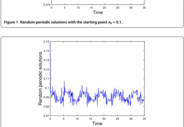
Figure 1 Random periodic solutions with the starting pointx0= 0.1.
Figure 2 Random periodic solutions with the starting pointx0= 0.15.
that we are working in a one-dimensional space of real numbers and consider the following SDE:
dXt= –Xtdt+
+Xt cost
dt+sint dWt, X() =x, ()
that is,
A= , f(t,Xt) = + Xt
cost, g(t) =sint.
Figure 3 Convergence of random periodic solutions with different starting points.
Figure 4 Convergence of random periodic solutions with different starting points.
We will run the simulation with the following meshes [, , ]:
s= –, t= , t= ., N=
to construct a random periodic solution with the starting point x= .. We generate Brownian trajectories in the following way:
W= , W(i+)t=Wit+ψi+,
where
ψi=N(,
√
t), i= , , . . . ,N.
Then we obtain the graphs for numerical approximations to random periodic solutions in the time interval [, ] as Figures and , respectively. As we see there exist random periodic phenomena with periodτ= π. That is, unlike the case in the deterministic sys-tems, random periodic solutions of SDE with the same starting point exist with a small dif-ference between two periods of time. However, the approximative structure of the graphs of the random periodic solutions with different starting points is preserved in the same period time. Random oscillation in the phase space leads to these phenomena due to the random noise pumped into this system constantly.
To check the convergence of numerical approximations, we plot the curves from differ-ent starting points at the timet= in the same graph. As we see from Figure , whose starting points arex= . andx= ., respectively, as time progresses, the trajectories become asymptotically close. Figure , whose starting points arex= . andx= ., respectively, also reflects the fact that whatever starting points we choose, as we move forward in time, the random periodic solutions arrive at the exact trajectories which de-pend on differentω∈, that is, random periodic solutions are stochastic processes and different for everyω∈. These results confirm that the numerical methods are efficient.
5 Conclusion
Finally, conclusions and future work are summarized. In this paper, the possibility of mean-square numerical approximations to random periodic solutions of SDEs is dis-cussed. The random Romberg algorithm is shown in detail. The results show that the method is effective and universal; numerical experiments are performed and match the results of theoretical analysis. In our further work, we will consider more simple and prac-tical methods which will be used to simulate a broader class of SDEs whose diffusion co-efficient is a function oftandx.
Competing interests
The author declares that he has no competing interests.
Author’s contributions
The author has read and approved the final manuscript.
Acknowledgements
The author would like to express his gratitude to Prof. Jialin Hong for his helpful discussion. This work is supported by NSFC (Nos. 11021101, 11290142, and 91130003).
Received: 7 April 2015 Accepted: 31 August 2015
References
1. Mao, X: Stochastic Differential Equations and Applications, 2nd edn. Ellis Horwood, Chichester (2008) 2. Milstein, G: Numerical Integration of Stochastic Differential Equations. Kluwer Academic, Dordrecht (1995) 3. Liu, B, Han, Y, Sun, X: Square-mean almost periodic solutions for a class of stochastic integro-differential equations.
J. Jilin Univ. Sci. Ed.51(3), 393-397 (2013)
4. Luo, Y: Random periodic solutions of stochastic functional differential equations. PhD thesis, Loughborough University, Department of Mathematical Sciences (2014)
5. Feng, C, Zhao, H, Zhou, B: Pathwise random periodic solutions of stochastic differential equations. J. Differ. Equ.251, 119-149 (2011)
6. Hong, J, Liu, Y: Numerical simulation of periodic and quasiperiodic solutions for nonautonomous Hamiltonian systems via the scheme preserving weak invariance. Comput. Phys. Commun.131, 86-94 (2000)
7. Liu, Y, Hong, J: Numerical method of almost periodic solutions for Lotka-Volterra system. J. Tsinghua Univ. (Sci. Technol.)40(5), 111-113 (2000)
8. Yevik, A, Zhao, H: Numerical approximations to the stationary solutions of stochastic differential equations. SIAM J. Numer. Anal.49(4), 1397-1416 (2011)
9. Arnold, L: Random Dynamical Systems, 2nd edn. Springer, Berlin (2003)
10. Khasminskii, R: Stochastic Stability of Differential Equations, 2nd edn. Springer, Berlin (2011)