Statistical framework for estimating GNSS bias

(1)

www.atmos-meas-tech.net/9/1303/2016/ doi:10.5194/amt-9-1303-2016

Statistical framework for estimating GNSS bias

Juha Vierinen1, Anthea J. Coster1, William C. Rideout1, Philip J. Erickson1, and Johannes Norberg2 1_{Haystack Observatory, Massachusetts Institute of Technology, Route 40 Westford, 01469 MA, USA} 2_{Finnish Meteorological Institute, P.O. Box 503, 00101 Helsinki, Finland}

Correspondence to: Juha Vierinen ([email protected])

Received: 26 July 2015 – Published in Atmos. Meas. Tech. Discuss.: 11 September 2015 Revised: 19 January 2016 – Accepted: 1 March 2016 – Published: 30 March 2016

Abstract. We present a statistical framework for estimating global navigation satellite system (GNSS) non-ionospheric differential time delay bias. The biases are estimated by examining differences of measured line-integrated electron densities (total electron content: TEC) that are scaled to equivalent vertical integrated densities. The spatiotemporal variability, instrumentation-dependent errors, and errors due to inaccurate ionospheric altitude profile assumptions are modeled as structure functions. These structure functions de-termine how the TEC differences are weighted in the linear least-squares minimization procedure, which is used to pro-duce the bias estimates. A method for automatic detection and removal of outlier measurements that do not fit into a model of receiver bias is also described. The same statisti-cal framework can be used for a single receiver station, but it also scales to a large global network of receivers. In addition to the Global Positioning System (GPS), the method is also applicable to other dual-frequency GNSS systems, such as GLONASS (Globalnaya Navigazionnaya Sputnikovaya Sis-tema). The use of the framework is demonstrated in prac-tice through several examples. A specific implementation of the methods presented here is used to compute GPS re-ceiver biases for measurements in the MIT Haystack Madri-gal distributed database system. Results of the new algorithm are compared with the current MIT Haystack Observatory MAPGPS (MIT Automated Processing of GPS) bias deter-mination algorithm. The new method is found to produce es-timates of receiver bias that have reduced day-to-day vari-ability and more consistent coincident vertical TEC values.

1 Introduction

A dual-frequency global navigation satellite system (GNSS) receiver can measure the line-integrated ionospheric electron density between the receiver and the GNSS satellite by ob-serving the transionospheric propagation time difference be-tween two different radio frequencies. Ignoring instrumental effects, this propagation delay difference is directly propor-tional to the line integral of electron density (Davies, 1965). This is derived, e.g., by Vierinen et al. (2014).

Received GNSS signals are noisy and contain system-atic instrumental effects, which result in errors when deter-mining the relative time delay between the two frequencies. The main instrumental effects are frequency-dependent de-lays that occur in the GNSS transmitter and receiver, arising from dispersive hardware components such as filters, ampli-fiers, and antennas. Loss of satellite signal can also cause unwanted jumps in the measured relative time delay and cause unwanted nonzero mean errors in the relative time de-lay measurement. Because line-integrated electron density is determined from this relative time delay, it is important to be able to characterize and estimate these non-ionospheric sources of relative time delay.

The non-ionospheric relative time delay due to hardware is commonly referred to as bias in the literature. For the specific case of GPS measurements, the bias is often separated into two parts ordered by the source of delay: satellite bias and receiver bias.

A GNSS measurement of relative propagation time delay difference including the line-integrated electron density ef-fect can be written as

m=b+c+

Z

S

(2)

where m is the measurement, b is the receiver bias, c is the satellite bias,Sis the path between the receiver and the satellite, Ne(s)is the ionospheric electron density at posi-tions, andξ is the measurement noise. The measurement is scaled to total electron content (TEC) units, i.e., 1016m−2, and therefore bias terms also have units of TEC. See Dyrud et al. (2008) and references therein for a more detailed dis-cussion.

For ionospheric research with GNSS receivers that per-form measurements of the per-form shown in Eq. (1), the quan-tity of interest is usually the three-dimensional electron den-sity function Ne(s). However, this quantity is challenging to derive from just GNSS measurements alone, as we only observe one-dimensional line integrals through the iono-sphere. The problem is an ill-posed inverse problem called the limited-angle tomography problem (Bust and Mitchell, 2008). The difficulty arises from the fact that line integrals are measured only at a small number of selected viewing angles, and this information is not sufficient to fully de-termine the unknown electron density distribution without making further assumptions about the unknown measurable

Ne(s). These assumptions often impose horizontal and verti-cal smoothness, as well as temporal continuity.

A considerable number of prior studies have attempted to solve this tomographic inversion problem in three dimen-sions for beacon satellites as well as for GPS satellites (see, e.g., Bust and Mitchell (2008) and references therein). Be-cause of the large computational costs and complexities as-sociated with full tomographic solvers, much of the practical research is done using a reduced quantity called the vertical total electron content (VTEC). As we will describe in more detail below, VTEC in essence results from a reduced param-eterization of the ionosphere that is used to simplify the to-mography problem and make it more well-posed. VTEC pro-cessing is only concerned with the integrated column density, and therefore the measurements are reported in TEC units.

The fundamental assumption for vertical TEC processing is that a slanted line integral measurement of electron den-sity can be converted into an equivalent vertical line integral measurement with a parameterized scaling factorv(α):

Z

V

Ne(s)ds≈v(α) Z

S

Ne(s)ds, (2)

where “V” is a vertical path, “S” is the associated slanted path,αis the elevation angle, andv(α)is the scaling factor that relates a slanted integral to a vertical line integral.

There are several ways that v(α)can be derived without resorting to full tomographic reconstruction of the altitude profile shape. Typically, the ionosphere above a certain ge-ographic point is assumed to be described with some verti-cal shape profilep(h)multiplied by a scalarNe(h)=Np(h). One example of an often-used shape profile is the Chapman

Figure 1. A scaled altitude profile model of the ionosphere assumes

that the ionosphere locally has a fixed horizontally stratified altitude profile shape multiplied by a scalar. This makes it possible to relate slanted line integrals to equivalent vertical line integrals using an elevation-dependent scaling factor called the mapping function. The pierce point is located where the ray pierces the peak of the electron density profile.

profile:

p(h)=exp1−z(h)−e−z(h), (3)

where z(h)=(h−hm)/H, hm is the peak altitude of the

ionosphere, andH is the scale height (Feltens, 1998). An-other example is a slab with exponential top and bottom side ramps as described by Coster et al. (1992) and Mannucci et al. (1998). Figure 1 depicts the geometry and profile shape assumptions in vertical TEC processing.

In more advanced models, the mapping function can be parameterized not only by elevation angle but also by factors such as time of day, geographic location, solar activity, and the azimuth of the observation ray. In practice, this can be done by using a first-principles ionospheric model to derive a more physically motivated mapping function.

Although the vertical TEC assumptions described above are not as flexible as a full tomographic model that attempts to determine the altitude profile, they provide model-to-data fits that are to first order good enough to produce measure-ments that are useful for studies of the ionosphere. The utility of this simplified model derives from the fact that it results in an overdetermined, well-posed problem that can be inverted with relatively stable results. The main practical difficulties in data reduction using the simplified model are estimating the receiver and satellite biasesbandc, as well as handling possible model errors.

(3)

the distribution of the differences of vertical TEC measure-ments is close to a zero mean normal random distribution, with the standard deviation increasing when the geographic distance between pierce points is increased, the temporal dis-tance is increased, or the elevation angle of the measurement is decreased.

We will show how this general statistical framework can be used to estimate biases in multiple special cases and fi-nally compare the newly presented method with an exist-ing bias determination scheme within the MIT Haystack MAPGPS (MIT Automated Processing of GPS) algorithm (Rideout and Coster, 2006). We will refer to this new method for bias determination as weighted linear least squares of in-dependent differences (WLLSID).

2 Receiver bias estimation

Let us denote Eq. (1) in a more compact form, but now with indexingito denote the index of a measurement,j to denote receiver, andkto denote the satellite:

mi=bj (i)+ck(i)+ni+ξi. (4)

Here ni is the line integral of electron density through the

ionosphere for measurementi. The receiver and satellite in-dex associated with measurementiis given byj (i)andk(i). Receiver noise is represented withξi.

Now consider subtracting slanted TEC measurements i

andi0, which are scaled with corresponding mapping func-tion valuesvi andvi0, which convert slanted TEC to equiva-lent vertical TEC. In this analysis, it does not matter if these measurements are associated with the same receiver or the same satellite, or even if they occur at the same time.

vimi−vi0m_i0=(v_in_i−v_i0n_i0)+v_ib_{j (i)}−v_i0b_{j (i}0₎

+vick(i)−vi0c_k(i0₎+v_iξ_i−v_i0ξ_i0 (5) This type of a difference equation has several benefits. If measurementsiandi0are performed at a time close to each otherti≈ti0 and have closely located pierce pointsx_i ≈x_i0, then we can make the assumption thatvini≈vi0n_i0, i.e., that the vertical TEC is similar.

We can statistically model this similarity by assuming that the difference of equivalent vertical line-integrated electron content between two measurements is a normally distributed random variable with variance

vini−vi0n_i0=_eξ_i,i0∼N 0, S_i,i0, (6)

whereSi,i0 is the structure function that indicates what we assume to be the variance of the difference of the two mea-surementsiandi0. This structure function would be our best guess of how different we expect these two measurements to be.

We assume the structure function depends on the follow-ing factors: (1) geographic distance between pierce points

di,i0= |x_i−x_i0|, (2) difference in time between when the measurements were madeτi,i0 = |t_i−t_i0|, (3) receiver noise of both measurementsξi+ξi0, and (4) modeling errors that are dependent on elevation anglesαiandαi0 of the measure-ments. The modeling errors in (4) are caused by inaccuracies in the assumption that we can scale a slanted measurement into an equivalent vertical measurement.

The following subsections describe the structure function behaviors for each dependent variable.

2.1 Geographic distance

In order to model the variability of electron density as a func-tion of geographic locafunc-tion, we assume the difference be-tween two measurements to be a random variable:

vini−vi0n_i0 ∼N 0, D(d_i,i0), (7)

where in this work we use √D(d)=0.5d in units of

(TECu/100 km). This implies that we assume the standard deviation of difference of two vertical TEC measurements to grow at a rate of 0.5 TEC units per 100 km of spacing be-tween pierce points.

For the results in this paper, we use the functional form above, but this can be improved in future work by a more complicated spatial structure functionD(xi, xi0, t_i, t_i0), which is a function of pierce point locationsxi andxi0, as well as the time of the measurementstiandti0. This function could for example be derived experimentally from vertical TEC measurements themselves. This would allow more ac-curate modeling of sunrise and sunset phenomena, as well as meridional and zonal gradients.

2.2 Temporal distance

Two measurements do not necessarily have to occur at the same time, but one would expect the two measurements to differ more if they have been taken further apart from one another. This difference can also be modeled as a normal ran-dom variable:

vini−vi0n_i0 ∼N 0, T (τ_i,i0), (8)

where T (τi,i0) is a structure function that statistically de-scribes the difference in vertical TEC from one measurement to the other when the time difference between the two mea-surements isτi,i0= |t_i−t_i0|.

In this work, we use√T (τ )=20τin units of TECu/hour. This makes the assumption that the standard deviation of the difference of two vertical TEC measurements grows at the rate of 20 TEC units for each hour.

(4)

2.3 Model and receiver errors

There are modeling errors that are caused by our assumption that we can scale a slanted line integral to a vertical line inte-gral as shown in Eq. (2). First of all, this assumption does not correctly take into account that the slanted path cuts through different latitudes and longitudes and thus averages vertical TEC over a geographic area. In addition to this, our mapping function assumes an altitude profile for the ionosphere that is hopefully close to reality, but never perfect. The ionosphere can have several local electron density maxima and can have horizontal structure in the form of, e.g., traveling ionospheric disturbances, or typical ionospheric phenomena such as the Appleton anomaly at the Equator or the ionospheric trough at high latitudes.

In addition to this, GNSS receivers often have difficulty with low-elevation measurements arising from near-field multi-path propagation, which is different for both frequen-cies. These errors can in some cases severely affect vertical TEC estimation and thus also bias estimation.

To first order, the errors caused by the inadequacies of the model assumptions or anomalous near-field propagation crease proportionally to the zenith angle. It is useful to in-clude this modeling error in the equations as yet another ran-dom variable. We have done this by assuming the elevation-angle-dependent errors to be a random variable of the follow-ing form:

vini−vi0n_i0∼N (0, E(α_i)+E(α_i0)) . (9)

HereE(αi)is the structure function that indicates the

mod-eling error variance as a function of elevation angle. In this work, we use a structure function where the variance grows rapidly as the elevation angle approaches the horizon, ex-pressed as√E(αi)=20(cosαi)4. This form penalizes lower

elevations more heavily.

The structure function that takes into account vertical TEC scaling errors and receiver issues at low elevations can also be determined from vertical TEC estimates, e.g., by doing a histogram of coincident measurements of vertical TEC:

resolution of the histogram on the α axis. Here the angle bracketsh·idenote a sample average operator.

3 Generalized linear least-squares solution

If we assume that all random variables in the structure func-tions of the previous section are independent random vari-ables, we can simply add them together to obtain the full structure function

Si,i0=D(d_i,i0)+T (τ_i,i0)+E(α_i)+E(α_i0). (11)

The differences in Eq. (5) can be expressed in matrix form as

m=Ax+ξ, (12) where A=      . .. ... ... ... ... ··· vi ··· vi ···

. .. ... ... ... . ..     −      . .. ... .._. .._. _{. .}. ··· vi0 ··· vi0 ···

. .. ... ... ... . ..      , (13)

with the measurement vector containing differences between vertically scaled measurements

m=[· · ·, vimi−vi0m_i0,· · ·]T, (14) and the unknown vectorxcontains the receiver and satellite biases

x=[b0,· · ·, bN, c0,· · ·, cM]T. (15)

Forx,N indicates the number of receivers andMindicates the number of satellites.

The random variable vector ξ∼N (0,6)has a diagonal covariance matrix defined by the structure function of each measurement pair used to form differences:

6=diag Si,i0,· · ·. (16) The theory matrix A forms the forward model for the mea-surements as a linear function of the receiver biases.

This type of a measurement is known as a linear statistical inverse problem (Kaipio and Somersalo, 2005), and it has a closed-form solution for the maximum-likelihood estimator for the unknownx, which in this case is a vector of receiver and satellite biases:

ˆ

x=(AT6−1A)−1AT6−1m. (17) This matrix equation is often not practical to compute di-rectly due to the typically large number of rows in A. How-ever, because the matrix A is very sparse, the solution can be obtained using sparse linear least-squares solvers. In this work, we use the LSQR package (Paige et al., 1982) for min-imizing|eAx−_em|2, whereeA andm_e are scaled versions of the matrix A and vectorm. Each row of A andmare scaled with the square root of the variance of the associated mea-surementp

Si,i0 in order to whiten the noise. In practice, this performs a linear transformation with matrix P that projects the linear system into a space where the covariance matrix is an identity matrix PT6P=I.

3.1 Outlier removal and bad receiver detection

(5)

residuals are larger than a certain threshold, they can be de-termined to be measurements that do not consistently fit the model, i.e., outliers.

Outliers can be caused by several different mechanisms. They can be of ionospheric origin, where vertical TEC gra-dients are sharper than our structure function expects them to be. They can also be simply caused by a loss of lock in the receiver, which can result in a large erroneous jump in slanted TEC.

These outlying measurements can be detected and re-moved by a statistical test, for example |eAxˆ−_em|>4σ, whereσ is the standard deviation of the residuals estimated withσ=median |eAxˆ−m|_e

. After the removal of problem-atic measurements, another improved maximum-likelihood solution, one not contaminated by outliers, can be obtained. The procedure for outlier removal can be repeated over sev-eral iterations to ensure that no problematic data are used for bias estimation.

4 Special cases

The previous section described the general method for esti-mating bias by using differences of slanted TEC measure-ments scaled by the mapping function. However, in practice this general form rarely needs to be used. In the following sections we describe several important and practical special cases, including known satellite bias, single receiver bias es-timation, and multiple biases for each receiver.

4.1 Known satellite bias

If satellite bias is known a priori to a good accuracy, then it can be subtracted from the measurements and the difference equation. This reduces Eq. (5) to

vimi−vi0m_i0=(v_in_i−v_i0n_i0)+v_ib_{j (i)}

−vi0b_{j (i}0₎+v_iξ_i−v_i0ξ_i0. (18) This form results in the same linear measurement equations, except that the satellite biases are not unknown parameters. In this case, the theory matrix will only have at most two nonzero elements for each row.

For GPS receivers, satellite biases are known to a good accuracy using a separate and comprehensive analysis tech-nique (Komjathy et al., 2005), and therefore this special case is appropriate for bias determination for GPS receivers. 4.2 Single receiver and known satellite bias

For the case that the satellite bias is known a priori and there is furthermore only one receiver, then the matrix only has one column with the unknown bias for the receiver.

This still results in an overdetermined problem that can be solved. The solution of this special case mathematically re-sembles a known analysis procedure that is often referred to as “scalloping” (P. Doherty, personal communication, 2003;

Carrano and Groves, 2006). This latter technique depends on the assumption that the concave or convex shape of all zenith TEC estimates collected by a single receiver observed over a 24 h period should be minimized. This same goal is obtained when time differences are minimized. The main difference in this work is that the statistical framework uses a structure function that weights differences of measurements based on time between the measurements, the elevation angle, and the pierce point distance.

Figure 2 shows an example receiver bias that is deter-mined using only data from a single receiver. In this case, time differences withτi,i0less than 2 h were used, in order to keep the number of measurements manageable. We also used differences of measurements between different satellites. A comparison of results with measurements obtained with the standard MAPGPS algorithm shows quite similar results be-tween the two techniques.

4.3 Multiple biases

There are several reasons for considering the use of multiple biases for the same satellite and receiver. This special case can also be handled by the same framework.

If there is a loss of phase lock on a receiver, this might re-sult in a discontinuity in the relative time-of-flight measure-ment, which appears as a discrete jump in the slanted TEC curve. Rather than attempting to realign the curve by assum-ing continuity, it is possible, usassum-ing our framework, to sim-ply assign an independent bias parameter to each continuous part of a TEC curve. As long as there are enough overlapping measurements, the biases can be estimated.

For GNSS implementations other than GPS, it is possible that satellite biases are not known or cannot be treated as a single satellite bias. For example, the GLONASS (Global-naya Navigazion(Global-naya Sputnikovaya Sistema) network uses a different frequency for each satellite, which means that any relative time delays between frequencies caused by the re-ceiver or transmitter hardware will most likely be different for each satellite–receiver pair. Because of this, it is natural to combine the satellite bias and receiver bias into a combined bias, which is unique for each satellite–receiver combination. Receiver biases are also known to depend on temperature (Coster et al., 2013), because dispersive properties of the dif-ferent parts of the receiver can change as a function of tem-perature. If an independent bias term is assigned to, e.g., each satellite pass, this also allows temperature-dependent effects to be accounted for, as a single satellite pass lasts only part of the day.

Multiple bias terms can be added in a straightforward man-ner to the model using Eq. (18). This is the same equation that is used for the known satellite bias special case. Here,bj (i)

(6)

Figure 2. Bias estimation using time differences of measurements obtained with a single receiver. Top panel shows the residuals of the

maximum likelihood fit to the data. The points shown with red are automatically determined as outliers and not used for determining the receiver bias. These mostly occur during daytime at low elevations. The center panel shows vertical TEC estimated with the original MAPGPS receiver bias determination algorithm, while the bottom panel shows vertical TEC measurements obtained using only time differences using the new method described in this paper, assuming constant receiver bias and known satellite bias. The VTEC results do not differ significantly.

necessarily need to have one unknown bias parameter; it can have many.

An example of a measurement where the same satellite is observed using a single receiver is shown in Fig. 3. In this case, the satellite is measured in the morning first, and dur-ing the pass there is a discontinuity in the TEC curve, most likely due to loss of lock. We give the measurements before ∼05:00 UTC and from∼05:00 to 06:00 UTC an indepen-dent bias termb0andb1. The same satellite is seen again in the evening at 19:00 UTC, and we again assign a new bias term to it:b2.

Another multiple-bias example is shown in Fig. 4, which displays measurements from 19 neighboring receivers in China. A few of these receivers have discrete jumps in the slanted TEC curves that make it impossible to assume a con-stant receiver bias during the course of the entire day. This can be seen as a poor fit using the standard MIT Haystack MAPGPS algorithm. When multiple bias terms are intro-duced (in the same way as depicted in Fig. 3), the measure-ments from these stations can be recovered.

5 Comparison

In order to test the framework in practice for a large network of GPS receivers, we implemented the framework described in this paper as a new bias determination algorithm for the MIT Haystack MAPGPS software, which analyzes data from over 5000 receivers on a daily basis. We used the MAPGPS

Figure 3. An example of a measurement of a single satellite

col-lected by a single receiver. A loss of phase lock occurs during the first pass of the satellite, resulting in two receiver biases for that pass (b0: blue curve;b1: green curve). During the next pass, a drift in the receiver bias could have occurred, so another receiver bias (b2: red curve) is determined when the satellite is measured during the end of the day.

(7)

Figure 4. Vertical TEC with satellite bias estimated using the current version of the MIT Haystack Observatory MAPGPS algorithm (Rideout

and Coster, 2006) shown above. Multiple receivers have problems with receiver stability, which makes the assumption of unchanging receiver bias problematic and causes the receiver bias determination to fail. Vertical TEC with receiver biases obtained using the multiple-biases assumption is shown below. The new method produces a more consistent baseline. The red dots show stations that are plotted. The algorithm uses all of the data from the 19 stations marked with orange and red dots. The stations marked with orange are used to assist in reconstruction by using a larger geographic area.

results obtained using the new bias determination algorithm with WLLSID.

When fitting for receiver bias, we assumed a fixed receiver bias for each station over 24 h. We also assumed a known satellite bias, which was removed from the slanted measure-ment. To keep the size of the matrix manageable, we selected sets of 11 neighboring receiver stations and considered each combination of measurements across receiver and satellites occurring within 5 min of each other as differences that went into the linear least-squares solution. For this comparison, we did not use time differences.

To estimate the goodness of the new receiver bias de-termination, we compared the method with the existing MAPGPS algorithm for determining receiver bias, which uti-lizes a combination of scalloping, zero-TEC, and differen-tial linear least-squares methods (Rideout and Coster, 2006; Gaposchkin and Coster, 1993). At latitudes higher than 70◦, the zero TEC method is used. This method finds the value of bias in such a way that the minimum value of TEC is 0. At low and midlatitudes scalloping is first used. Scalloping finds the bias by finding the optimally flat vertical TEC±2 h around local noon. After finding the bias with either zero TEC or scalloping, the values are refined by using the dif-ferential TEC method described by Gaposchkin and Coster (1993).

5.1 Self-consistency comparison

As a measurement of goodness, we used the absolute dif-ference between two simultaneous geographically coincident measurements of vertical TEC|vini−vi0n_i0|. The two mea-surements were considered coincident if the distance be-tween the pierce points was less than 50 km and the measure-ments occurred within 30 s of each other. We also required that the two measurements were not obtained using the same receiver. As a figure of merit, we used the mean value of the absolute differences:

F = 1

N X

i6=i0

|vini−vi0n_i0|. (19)

This figure of merit measures the self-consistency of the measurements, i.e., how well the vertical TEC measurements obtained with different receivers agree with one another. The smaller the value, the more consistent the vertical TEC mea-surements are.

(8)

Figure 5. Probability density function and cumulative density functions for 192 360 coincidences where vertical TEC was measurement

within the same 30 s time interval and have pierce points less than 50 km apart from one another. The new method (labeled as WLLSID) has significantly more<1 TEC unit differences than the old method.

units, and the WLLSID method has a figure of merit of 1.62 TEC units, which is about 30 % better.

The probability density function and cumulative density function estimates for the coincident vertical TEC differ-ences are shown in Fig. 5. The new method results in signifi-cantly more<1 TEC unit differences than the old method. It is evident from the cumulative distribution function that both methods also result in some coincidences that are in large dis-agreement with each other. The result occurs at least in part due to our inclusion of elevations down to 10◦in the com-parison, and it is therefore expected that some low-elevation measurements will be significantly different from one an-other.

5.2 Receiver bias day-to-day change

We also investigated receiver bias variation from day to day. We arbitrarily selected two consecutive quiet days: days 140 and 141 of 2015. We calculated the sample mean day-to-day change in receiver bias across all receivers:

δb= 1

N

X

i=0

bi,140−bi,141, (20)

whereN is the number of receiver. In addition to this, we calculated the standard deviation using sample variance:

σb=

v u u t

1

N−1

N

X

i=0

(bi,140−bi,141)−δb 2

. (21)

For the MAPGPS method, we found overall thatδb= −0.2± 0.05(2σ )TEC units andσb=1.6 TEC units. With the new

WLLSID method, we found thatδb=0.02±0.05(2σ )TEC units andσb=1.3 TEC units. This indicates not only that

the day-to-day variability is slightly smaller with the new method but also that the old method has a statistically signifi-cant nonzero mean day-to-day change in receiver bias, which is not seen with the new method. When the data are broken down into high and equatorial latitudes, the result is similar. 5.3 Qualitative comparison

In order to qualitatively compare the MAPGPS bias deter-mination method with the WLLSID method, we produced a global TEC map with the WLLSID method and the exist-ing MAPGPS bias determination method. The processexist-ing in-volved with making these TEC maps is described by Rideout and Coster (2006).

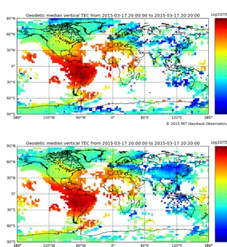
To highlight the differences between the two methods, we chose a geomagnetic storm day (17 March 2015), where we would expect large gradients and more issues with data qual-ity. Because of this, the bias determination problem is more challenging than on a geomagnetically quiet day.

(9)

ioniza-Figure 6. Global TEC map produced using two different methods for the St. Patrick’s Day storm on 17 March 2015. Top: a map produced

with the MAPGPS method. Bottom: a map produced with the new WLLSID bias determination method.

tion drift (SAID) stretching from Asia to northern Europe is much more clearly seen with the new method. Probably due to the strong gradients associated with the storm, the old method fails to derive good bias values for a large number of receivers in China, resulting in negative TEC values, which are not plotted. The new method finds these values of bias more reliably.

The polar regions have slightly more TEC when using WLLSID. This is because the MAPGPS uses the zero-TEC method for receiver bias determination at high latitudes, whereas the WLLSID method is applied in the same way everywhere.

6 Conclusions

In this paper, we describe a statistical framework for esti-mating bias of GNSS receivers by examining differences be-tween measurements. We show that the framework results in a linear model, which can be solved using linear least squares. We describe a way that the method can be effi-ciently implemented using a sparse matrix solver with very

low memory footprint, which is necessary when estimating receiver biases for extremely large networks of GNSS re-ceivers.

We compare our method for bias determination with the existing MIT Haystack MAPGPS method and find the new method results in smaller day-to-day variability in receiver bias, as well as a more self-consistent vertical TEC map. Qualitatively, the new method reproduces the same general features as the existing MAPGPS method that we compared with, but it is generally less noisy and contains fewer outliers. The weighting of the measurement differences is done us-ing a structure function. We outline a few ways to do this, but these are not guaranteed to be the best ones. Future improve-ments to the method can be obtained by coming up with a better structure function, which can possibly be determined from the data themselves, e.g., using histograms, empirical orthogonal function analysis, or similar methods.

(10)

mea-surements, obviously all the possible differences cannot be included in the model. In this study, we only explored two types of differences: (1) differences between geographically separated, temporally simultaneous measurements obtained with tens of receivers located near each other and (2) differ-ences in time less than 2 h performed with a single receiver. There are countless other possibilities, and it is a topic of future work to explore what differences to include to obtain better results.

We describe several important special cases of the method: known satellite bias, single receiver and known satellite bias, and the case of multiple bias terms per receiver. The first two are applicable for GPS receivers, and the last one is appli-cable to GLONASS measurements, as well as measurements where a loss satellite signal has caused a step-like error in the TEC curve.

Acknowledgements. GPS TEC analysis and the Madrigal distributed database system are supported at MIT Haystack Observatory by the activities of the Atmospheric Sciences Group, including National Science Foundation grants AGS-1242204 and AGS-1025467 to the Massachusetts Institute of Technology. Vertical TEC measurements using the standard MAPGPS algorithm are provided free of charge to the scientific community through the Madrigal system at http://madrigal.haystack.mit.edu.

Edited by: M. Portabella

References

Bust, G. S. and Mitchell, C. N.: History, current state, and future di-rections of ionospheric imaging, Rev. Geophys., 46, 1–23, 2008. Carrano, C. S. and Groves, K.: The GPS Segment of the AFRL-SCINDA Global Network and the Challenges of Real-Time TEC Estimation in the Equatorial Ionosphere, Proceedings of the 2006 National Technical Meeting of The Institute of Navigation, Mon-terey, CA, 2006.

Coster, A., Williams, J., Weatherwax, A., Rideout, W., and Herne, D.: Accuracy of GPS total electron content: GPS re-ceiver bias temperature dependence, Radio Sci., 48, 190–196, doi:10.1002/rds.20011, 2013.

Coster, A. J., Gaposchkin, E. M., and Thornton, L. E.: Real-time ionospheric monitoring system using the GPS, MIT Lincoln Lab-oratory, Technical Report, 954, 1992.

Davies, K.: Ionospheric Radio Propagation, National Bureau of Standards, 278–279, 1965.

Dyrud, L., Jovancevic, A., Brown, A., Wilson, D., and Ganguly, S.: Ionospheric measurement with GPS: Receiver techniques and methods, Radio Sci., 43, RS6002, doi:10.1029/2007RS003770, 2008.

Feltens, J.: Chapman profile approach for 3-D global TEC represen-tation, IGS Presenrepresen-tation, 1998.

Gaposchkin, E. M. and Coster, A. J.: GPS L1-1,2 Bias Determina-tion, Lincoln Laboratory Technical Report, 971, 1993.

Kaipio, J. and Somersalo, E.: Statistical and Computational Inverse Problems, Springer, New York, USA, 2005.

Komjathy, A., Sparks, L., Wilson, B. D., and Mannucci, A. J.: Au-tomated daily processing of more than 1000 ground-based GPS receivers for studying intense ionospheric storms, Radio Sci., 40, RS6006, doi:10.1029/2005RS003279, 2005.

Mannucci, A. J., Wilson, B. D., Yuan, D. N., Ho, C. H., Lindqwister, U. J., and Runge, T. F.: A global mapping technique for GPS-derived ionospheric total electron content measurements, Radio Sci., 33, 565–582, 1998.

Paige, C. C. and Michael, A.: Saunders, LSQR: An algorithm for sparse linear equations and sparse least squares, ACM Transac-tions on Mathematical Software (TOMS), 8, 43–71, 1982. Rideout, W. and Coster, A.: Automated GPS processing for global

total electron content data, GPS Solutions, 10, 219–228, 2006. Vierinen, J., Norberg, J., Lehtinen, M. S., Amm, O., Roininen, L.,