http://www.sciencepublishinggroup.com/j/cse doi: 10.11648/j.cse.20180201.12
Comparative Analysis of PID, IMC, Infinite H Controllers for
Frequency Control in Hydroelectric Plants
Korassaï
1, *, Yeremou Tamtsia Aurelien
2, Haman Djalo
1, Ngaleu Gildas Martial
2,
Ndzana Jean Calvin
21
Faculty of Science, University of Ngaoundere, Ngaoundere, Cameroon
2
Faculty of Industrial Engineering, University of Douala, Douala, Cameroon
Email address:
*
Corresponding author
To cite this article:
Korassaï, Yeremou Tamtsia Aurelien, Haman Djalo, Ngaleu Gildas Martial, Ndzana Jean Calvin. Comparative Analysis of PID, IMC, Infinite H Controllers for Frequency Control in Hydroelectric Plants. Control Science and Engineering. Vol. 2, No. 1, 2018, pp. 16-26.
doi: 10.11648/j.cse.20180201.12
Received: November 23, 2018; Accepted: December 18, 2018; Published: January 14, 2019
Abstract: One of the most important criteria for the stability of electrical networks, is the frequency of the voltage produced.
This frequency is subjected to the hazards of the load connected to the turbo generator group. Indeed, the balance of the frequency results from the balance between active power produced by the turbo alternator group and power demanded by the load connected to the network. This paper presents a comparative study of three methods of regulation to solve the problem of frequency fluctuations in hydroelectric plants: modified Proportional–Integral–Derivative (PID) control, Internal Model Control (IMC) and Infinite Horizon (H∞) Control. Simulation model in the presence of these has been established in Matlab / Simulink. The results of the simulation have subsequently revealed their robustness, which demonstrates once again their reliability.Keywords: Electrical Network, Frequency, Modified PID Control, Internal Model Control, Infinite Horizon Control
1. Introduction
The role of a frequency control system of a power plant is to ensure a balance between the energy produced and the energy consumed by the users, connected to the network. The efficiency of such a system can be estimated through its ability to respond quickly to user demand, without causing instabilities in the installation. Despite the desire to control consumption, demand tends to grow higher, not only in quantity but also in the quality of the service, especially in the developing countries. It is most often characterized by a high growth of demand, due to rampant urbanization and recurrent aging production equipment, causing variations in the parameters of the control system. In order to provide a long-term solution to this problem, numerous studies have been conducted on automatic controllers in recent decades [1-8].
The main contributions of this work are:
1.The identification of the parameters of the first-order model, of the frequency regulation system of a
turbo-generator group at the Songloulou hydroelectric plants in Cameroon:
2. The synthesis of an adaptive internal model command for the system.
3. The synthesis of an infinite horizon command for the system.
In this context, it will deal with the structure of the control system that allows it to follow the requirements of globalization in terms of adaptation (stability, speed, accuracy).
2. Related Work
The block diagram of a hydroelectric plant including the speed control system is shown in Figure 1 below, [9-10]:
Figure 1. Block diagram of the speed control system for a hydroelectric power plant.
The Songloulou hydropower plant has the following characteristics: Francis Turbine (P=49.5MW, D=4.55m), synchronous alternator (S = 57MVA, Cos (φ) = 0.85, U = 10.3kV, D = 9.20m, J = 8800 t / m2), MIPREG controller 600c.
The modeling of the frequency regulation system of a turbo-generator group of the Songloulou hydroelectric plant in Cameroon was presented [11]. It have thus been able to obtain the transfer functions of the different organs entering the control chain; the active power chain and therefore, the load has also been presented. Subsequently it synthesized a PID corrector by the method of Ziegler and Nichols that it optimized [12]. Figure 2 shows the graph of the open-loop transfer function (for a 0.5mA step-type input) of the system and Figure 3 shows the comparative index responses of the system after correction.
Figure 2. Open loop system response to a 0.5A step type input.
Figure 3. Calculated PID and Modified PID index responses.
3. New Contribution
3.1. Identification of the Parameters of the First Order Model of the System
In order to identify the parameters of the first order system, the frequency control system of a turbo alternator group of the Songloulou plant, and in the absence of the experimental results, often used the results obtained on the virtual laboratory of Matlab (see figure 2). Given the large number of indices, the Matlab toolbox was used to obtain the most accurate first order model possible using the least squares method.
The model thus obtained has the function of transfer:
( )
100.085 1 42.589 M ss
=
+ (1)
Figure 4 shows the responses of the open-loop system (in blue) and the first-order model (in red) to a step-type input of 0.5mA (idling conditions).
Figure 4. Comparing growths of open-loop system responses and model.
There is a good correlation between the system and the proposed first order model.
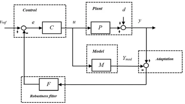
3.2. Synthesis of the Internal Model Control (IMC)
same dynamics as its model, they are generalized through a presentation starting from four well-defined functional blocks
[13-15]. Its block diagram is shown in Figure 5.
Figure 5. Block diagram of the internal model control.
Where yrefis the set point, e is the modified set point, u is the controller output, d is the disturbance and Ymod is the process model output.
From this block diagram often deduce the equations governing the system:
(
)
ref
e y PCe MCe d
y PCe d
= − − +
= +
(2)
From where
(
)
1(
)
1 ref 1
CP CM
y y d
C P M C P M
−
= +
+ − + − (3)
From equation (3), it appears that to remove any perturbation d, one must have at all times [13]:
1−CM =0 (4)
Is:
1
1
C M
M
−
= = (5)
Once the above condition is verified, the result always get:
ref
y=y (6)
If P is stable (which is the case here), and if the model is perfect (P = M), then the system controlled by the internal model structure is stable if and only if the corrector C is stable. This implies that the transfer function of the model is invertible and that its inverse is feasible, which is not always the case; the model being first-rate, should have:
( )
1
M
M
K M s
s
τ =
+ (7)
Where KM is the static gain, is the time constant. The corrector that would be propose has the function of transfer:
( )
1 MM
s C s
s K
τ + =
+ (8)
A robustness filter is generally introduced in the feedback loop which makes it possible to avoid performance degradation in the presence of a too large difference between P and M [16].
The simplest filters are of the form [17]:
( )
(
)
1
1 F n
F s
s
τ =
+ (9)
and
( )
(
)
1 1 F n F n s F s s τ τ + =+ (10)
Where is a tuning parameter for the speed of the closed loop, n is the order of the process.
However, there chose to use a filter of the following form (with b> 1) to avoid the appearance of oscillations in the control when the system reacts quickly:
( )
11 F F s F s k s τ τ + =
+ (11)
Where k is the any constant.
The correct choice of filter parameters allows us to act on the speed and accuracy of the process compared to its model, to control the robustness and also to soften the order. In addition, this configuration allows us to choose a model that is faster than the process, without degrading system performance and thus, improving speed and control.
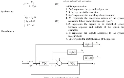
The transfer function of the fast model is:
' ' 1 M M K M s τ =
+ (12)
By choosing: ' 4 0.75 1.25 M M F k
τ
τ
τ
= = = (13) Should obtain:( )
( )
( )
100.085 1 10.7 10.7 1 100.085 0.75 1 0.9375 1 M s s s C s s s F s s = + + = + + = + (14)3.3. Synthesis of Infinite H Control
3.3.1 Formulation and Resolution of the Problem Command
The robust control H2 or H∞ (advanced frequency control) was born from the search for a better formalization of the specifications by mathematical criteria, whose effective resolution allows to synthesize a corrector satisfying these specifications [18].
The standard H∞ robust control problem is defined as follows (Figure 7) [19]:
Figure 7. Representation in "standard form" of a system for synthesis H∞, (a) with corrector, (b) with uncertainty.
In this representation:
1.P (s): represents the generalized process. 2.K (s): represents the corrector.
3.∆ (s): represents the modeling of uncertainties.
4.W: represents the exogenous entries of the system (entries to follow and disturbances to reject).
5.Z: represents the signals to be controlled (errors between setpoints and outputs of the system for example).
6.Y: represents the outputs accessible to the system measurement.
7.U: represents the control signals of the process.
Figure 8. Diagram of synthesis H∞ 4 blocks.
a formulation based on three weighting functions is generally used because it is sufficient to solve a large part of the synthesis problems. This formulation is based on the diagram that is represented below called 4 blocks [20-21].
The 4-block summary scheme is based on the use of three weighting functions.
For this, the diagram of Figure 8 is considered, in which the error ε is weighted by the filter W1 (s), the command u by W2 (s), and the disturbance input b by W3 (s) [21].
Considering r and b as inputs and e1 and e2 as performance signals, the standard H∞ problem is to look for a number.
γ > 0 and a corrector K (s) stabilizing the looped system, and ensuring : γ> 0 and a corrector K (s) stabilizing the looped system, and ensuring [21]:
( )
M s∞ < γ (15)
With
( )
( )
( ) ( )
( )
1 2
e s r s
M s
e s b s
=
(16)
( )
( ) ( ) ( )
1( ) ( )
1( ) ( ) ( ) ( )
( ) ( ) ( )
32 2 3
W s S s W s S s G s W s
M s
W s K s S s W s T s W s
=
(17)
( )
( ) ( )
( )
( )
1 1 1 S sG s K s
T s S s
= + = − (18)
Where [18-19] [21-22]:
( )
(
)
( )
( )
(
)
( )
1 3 1 W s S sT s W s
σ σ ≥ ≤ (19)
σ
Represents the maximum singular value.The filters W1 (s), W2 (s) and W3 (s) thus makes it possible to dynamically limit (to the value of γ near) the various transfers S, KS, SG and T.
Generally, these filters are chosen as follows [19-22]: 1.The template on S is chosen to ensure precision
objectives. For this reason it is necessary to choose a high-pass filter with a lower gain at low frequencies. The heartbeat for which the template intersects the 0dB axis can be interpreted as the minimum bandwidth desired for servo control. The value of the high frequency mask limits the maximum of the frequency response of S, which imposes a module margin at least equal to its inverse. At high frequencies no constraint is imposed on S.
2.The template on KS
(
W2−1( )
s)
is chosen as a low-pass filter with a low gain at high frequencies, beyond the bandwidth set for servo control. This constraint is even more severe than the attenuation requested intervenesclose to the cutoff pulse of the open loop. At low frequencies no constraint is imposed on KS.
3. The template on SG depends on the two filters W1 (s) and W3 (s). In some cases, just choose W3 (s) constant, to adjust the attenuation at low frequencies (introduction of an integral effect in the corrector). Moreover, in medium frequencies the behavior of SG can be modified using W3 (s). This may be useful for obtaining proper transient behavior in response to a disturbance.
4. The template on KSG is imposed by the previous choices.
This 4-block methodology requires the adjustment of three weighting functions (W1, W2 and W3), which can be tricky for some complex control systems.
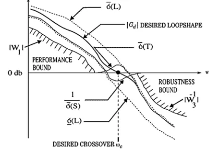
Equation (19) gives the notion of "loop shaping"(loop formation) for the synthesis of a robust controller H∞, in order to satisfy the compromise "robustness performance" (Figure 9) [18].
Figure 9. Loop shaping specifications.
These considerations illustrate the unavoidable trade-off of single-variable linear automatism, accuracy / stability: any increase in singular values improves performance at low frequencies, but can lead to instability. The best compromise implies that in the vicinity of the cutoff frequency, the singular values are quite close to each other [20].
Once the functions W1, W2 and W3 have been chosen, the resolution of the standard control problem is done by means of the GLOVER - DOYLE algorithm and the resolution of the Riccati equations [18]. That will not discuss here this resolution more or less complex, since the corrector can now be obtained directly from Matlab using the "mixsyn" command.
Note that this controller is of the same order as the system augmented by the weighting functions [18].
3.3.2. Synthesis of the Regulator H∞
On the basis of the criteria previously established, there choose as weighting functions:
( )
1 100 0.05 0.0001 s W s s + =( )
2 0.4
0.05 1 s W s
s
=
+ (21)
( )
3 0.01
W s = (22)
4. Simulation Results
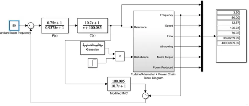
In this paper, the simulation model of the power plant in the presence of different controllers has been established in
MATLAB/Simulink, as shown in figure 10 for the model of the power plant in the presence of the modified PID, figure 11 for the model of the power plant in the presence of the modified IMC and figure 12 for the model of the power plant in the presence of the infinite H controller. Inside each turbine / alternator block, has added the power chain block to introduce the disturbance.
Figure 10. Model of the power plant in the presence of the modified.
Figure 11. Model of the power plant in the presence of the Modified IMC controller.
4.1. In the Absence of Disturbances
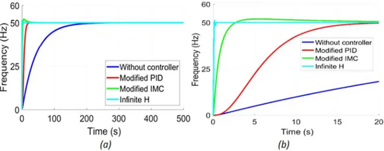
As simulate for 500 seconds, the response of the system at a step of 0.5 mA without corrector and with corrector (Figure 13); this simulation corresponds to the conditions of idling. The frequency is well maintained at the value of 50 Hz. It should be noted that the startup phase is subjected to a procedure that does not take into account the correctors, which therefore have no interest during this phase.
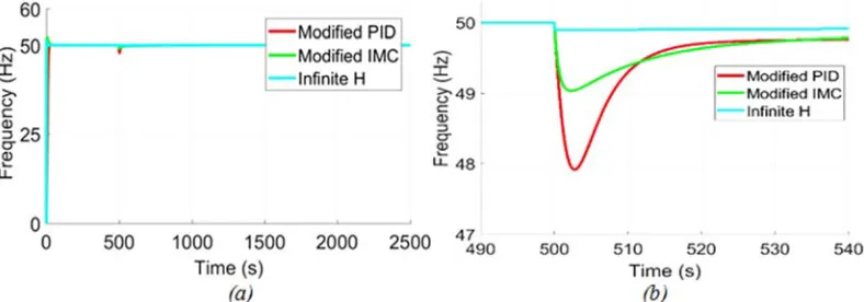
4.2. In the Presence of Disturbances
As simulate during 2500s the response of the system to a load disturbance (demand of 48 MW power) appearing at 500s, under a gross drop height of 39 m.
In the absence of a corrector, the frequency drops to 1.333 Hz for a speed of w = 3.199 tr/min (Figure 12). In the presence of the controllers, the disturbance is quickly eliminated. Figure 15 and Figure 16 shows the evolution of the winnowing associated with each controller and Figure 17 highlights the load torque and motor torque associated with each controller.
That introduce the actual operating conditions: the nominal load is 48MW and white Gaussian noise (average 48MW, variance 10MW). The results are shown in Figure 18. The
frequency in all three cases is always maintained around 50 Hz.
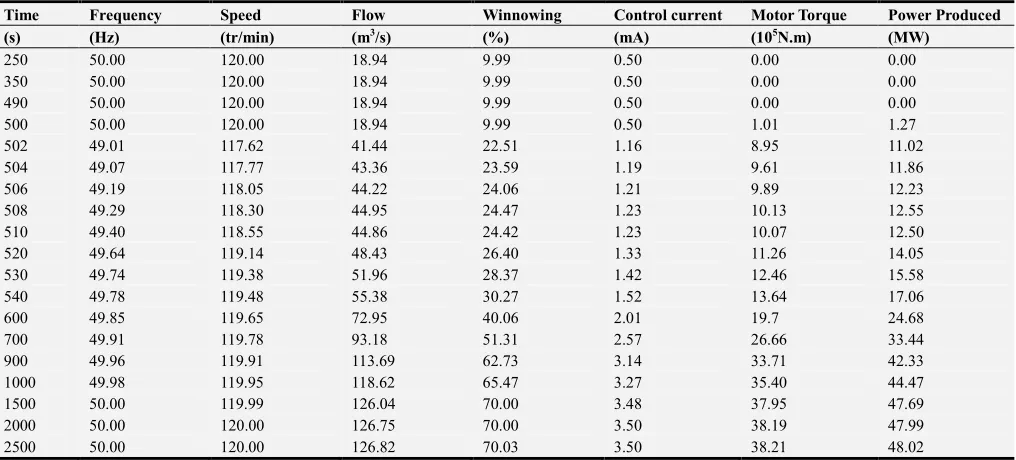
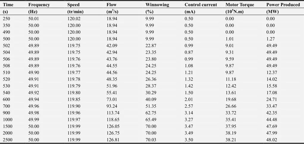
Tables 1, 2 and 3 present the corrected frequencies, the water flow, the winnowing, the servo valve control currents, the motor torques and the power generated by the turbo-generator for the different types of correctors proposed with disturbance (demand of 48MW power). While noted that 2 seconds after a disturbance, the frequency when controlled with the modified PID controller, fell below the normal range ([48-52] Hz) and is at 47.96 Hz. At the same time, it is 49.01 Hz with the modified IMC controller and 49.89 with the Infinite H controller. It is realized that for small variations around the nominal operating point, all chosen controllers are suitable.
However, when these disturbances become important, the PID is no longer effective, and the infinite H controller is more robust than the IMC controller.
In addition, these tables show the flexibility of the different correctors compared to the constraints of the mechanical organs. We realize the different regimes are imposed by the PID command, regimes that are slightly mitigated by the IMC command, whereas, the infinite H command imposes less varied regimes.
Figure 13. Frequency versus time curves, unladen (a) normal, (b) zoom.
Figure 15. Frequency output of the alternator with controller, (a) normal, (b) zoom.
Figure 16. Winnowing at the inlet of the turbine, (a) normal, (b) zoom.
Figure 18. Power demanded by the load (a), frequency with PID corrector (b), with IMC corrector (c), with infinite H corrector (d).
Table 1. Parameters of the hydroelectric power plant with Modified PID controller.
Time Frequency Speed Flow Winnowing Control current Motor Torque Power Produced
(s) (Hz) (tr/min) (m3/s) (%) (mA) (105N.m) (MW)
250 50.00 120.00 18.94 9.99 0.50 0.00 0.00
350 50.00 120.00 18.94 9.99 0.50 0.00 0.00
490 50.00 120.00 18.94 9.99 0.50 0.00 0.00
500 50.00 120.00 18.94 9.99 0.50 1.01 1.27
502 47.96 115.10 37.34 20.23 1.14 7.67 9.25
504 48.03 115.27 45.33 24.68 1.26 10.53 12.71
506 48.56 116.55 46.57 25.37 1.27 10.85 13.25
508 49.00 117.60 46.50 25.33 1.27 10.73 13.22
510 49.31 118.33 45.71 24.89 1.25 10.39 12.87
520 49.71 119.31 48.39 26.38 1.33 11.23 14.03
530 49.76 119.42 51.91 28.34 1.42 12.44 15.56
540 49.77 119.45 55.35 30.26 1.52 13.63 17.05
600 49.83 119.59 72.94 40.05 2.01 19.7 24.67
700 49.89 119.74 93.16 51.30 2.57 26.67 33.44
900 49.96 119.90 113.68 62.72 3.14 33.71 42.33
1000 49.97 119.94 118.61 65.46 3.27 35.4 44.46
1500 50.00 119.99 126.04 70.00 3.48 37.95 47.68
2000 50.00 120.00 126.75 70.00 3.50 38.19 47.99
2500 50.00 120.00 126.82 70.03 3.50 38.21 48.02
Table 2. Parameters of the hydroelectric power plant with Modified IMC controller.
Time Frequency Speed Flow Winnowing Control current Motor Torque Power Produced
(s) (Hz) (tr/min) (m3/s) (%) (mA) (105N.m) (MW)
250 50.00 120.00 18.94 9.99 0.50 0.00 0.00
350 50.00 120.00 18.94 9.99 0.50 0.00 0.00
490 50.00 120.00 18.94 9.99 0.50 0.00 0.00
500 50.00 120.00 18.94 9.99 0.50 1.01 1.27
502 49.01 117.62 41.44 22.51 1.16 8.95 11.02
504 49.07 117.77 43.36 23.59 1.19 9.61 11.86
506 49.19 118.05 44.22 24.06 1.21 9.89 12.23
508 49.29 118.30 44.95 24.47 1.23 10.13 12.55
510 49.40 118.55 44.86 24.42 1.23 10.07 12.50
520 49.64 119.14 48.43 26.40 1.33 11.26 14.05
530 49.74 119.38 51.96 28.37 1.42 12.46 15.58
540 49.78 119.48 55.38 30.27 1.52 13.64 17.06
600 49.85 119.65 72.95 40.06 2.01 19.7 24.68
700 49.91 119.78 93.18 51.31 2.57 26.66 33.44
900 49.96 119.91 113.69 62.73 3.14 33.71 42.33
1000 49.98 119.95 118.62 65.47 3.27 35.40 44.47
1500 50.00 119.99 126.04 70.00 3.48 37.95 47.69
2000 50.00 120.00 126.75 70.00 3.50 38.19 47.99
Table 3. Parameters of the hydroelectric power plant with Infinite H controllers.
Time Frequency Speed Flow Winnowing Control current Motor Torque Power Produced
(s) (Hz) (tr/min) (m3/s) (%) (mA) (105N.m) (MW)
250 50.01 120.02 18.94 9.99 0.50 0.00 0.00
350 50.00 120.00 18.94 9.99 0.50 0.00 0.00
490 50.00 120.00 18.94 9.99 0.50 0.00 0.00
500 50.00 120.00 18.94 9.99 0.50 1.01 1.27
502 49.89 119.75 42.09 22.87 0.99 9.01 49.49
504 49.89 119.75 42.94 23.35 0.87 9.31 49.49
506 49.89 119.76 43.76 23.80 0.99 9.59 49.49
508 49.89 119.76 44.55 24.25 1.08 9.87 49.49
510 49.90 119.77 44.56 24.25 1.21 9.87 12.37
520 49.91 119.78 48.35 26.36 1.32 11.18 14.02
530 49.91 119.79 51.96 28.37 1.42 12.42 15.58
540 49.92 119.80 55.41 30.29 1.50 13.61 17.08
600 49.94 119.85 73.01 40.09 2.01 19.68 24.71
700 49.96 119.90 93.24 51.35 2.57 26.66 33.47
900 49.98 119.96 113.74 62.75 3.14 33.72 42.35
1000 49.99 119.97 118.65 65.49 3.27 35.41 44.48
1500 50.00 119.99 126.05 70.00 3.47 37.95 47.69
2000 50.00 119.99 126.75 70.00 3.49 38.19 47.99
2500 50.00 119.99 126.81 70.03 3.50 38.21 48.02
5. Conclusion
In this paper, the speed control system of a group of Songloulou hydroelectric plant was modeled and simulated. The different simulations showed a good similitude between the real system and its model. Often chose a modified PID corrector to simulate the current operation of the control system, then two robust correctors, IMC and Infinite H for its improvement. Simulations carried out under the Matlab / Simulink environment have corroborated further predictions that a robust corrector (in this case H infinite) would be more suitable for frequency control in Songloulou. However, new perspectives open up for the rest of this work. There are thinking about the sizing and implementation of a ballast resistor to more effectively buffer sudden large amplitude variations.
References
[1] Matei Vinatoru, Eugen Iancu, Camelia Maican, and Gabriela Canureci. Control System for Kaplan Hydro-Turbine. 4th WSEAS/IASME International Conference on dynamical systems and control, Corfu, Greece, October 26-28, 2008. [2] IEEE Committee Report, Hydraulic Turbine and Turbine
Control Models for System Dynamic Studies, IEEE Transaction on Power Systems, vol. 7, no. 1, pp. 167-179, Febuary 1992.
[3] Ayele Nigussie Legesse, Mengesha Mamo. Application of a Stepper Motor tothe Frequency Control of a Mini Hydropower Plant.Electrical and Power Engineering Frontier, Sep. 2013, Vol. 2 Iss. 3, PP. 59-63.
[4] Hannet L. N., Fardanesh B., Field test to validate hydroturbine-governor model structure and parameters, IEEE Transaction on Power Systems, vol. 9, 1994, pp. 1744-1751.
[5] Arnaurovic D.B., Skataric D.M, Suboptimal design of Hydroturbine governors, IEEE Transactions on energy Conversion, Vol. 6/3, 1991.
[6] Jin Z., Manisa P., Saifur R., Xu L. A Frequency Regulation Framework for Hydro Plants to Mitigate Wind Penetration Challenges. IEEE Transaction on Sustainable Energy. 2016. [7] Ghazanfar S. Power System Stabilizer Application for load
Frequency Control in Hydro-Electric Power Plant. International Journal of theoretical and Applied Mathematics. Vol.3, No.4, 2017, pp 148-157.
[8] Anaza S. 0., Abdulazeez M. S., Yisah Y. A., Yusuf Y. O., Salawu B. U, Momoh S. U. Micro Hydro-Electric Energy Generation – An Overview. American Journal of Engineering Reseach (AJER), Vol. 6, 2017, pp 05-12
[9] Zohra Zidane, Mustapha Ait Lafkih, Mohamed Ramzi. Application of Multivariable Predictive Control in a Hydropower Plant. Journal of Automation and Control, 2013, Vol. 1, No. 1, 26-33, Received February 07, 2013; Revised November 12, 2013; Accepted December 20, 2013.
[10] S. Boyd and C. Barrat. Linear Controller Design: Limits of Performance. Prentice Hall, 1991.
[11] A.Yeremou Tamtsia, J.M. Nyobe Yome, G. M. Ngaleu, J. C. Ndzana. Contrôle de la fréquence dans une centrale de production d’énergie électrique. Sciences, Technologies et Développement, Edition spéciale, ISSN 1029 – 2225 - e - ISSN 2313 – 6278, pp39-44, Juillet 2016.
[12] LE Hoang Bao, "Contribution aux méthodes de synthèse de correcteurs d’ordres réduits sous contraintes de robustesse et aux méthodes de réduction de modèles pour la synthèse robuste en boucle fermée". PhD thesis. Institut National Polytechnique de Grenoble - INPG, 2010.
[14] Guolian H., Yuzhao H., Huan D., Jianhua Z. Xiaobin Z. Design of Internal Model Controller Based on ITAE Index and Its Application in Boiler Combustion Control System. IEEE 12th ICIEA. 2017: 2078-2083.
[15] Nian L., Feng W., Yu Y. Design and Simulation Analysis for An Internal Model Controller of Speed Loop. IEEE 29th CCDC. 2017: 5056-5059.
[16] L. Saidi, “Commande à modèle interne : Inversion et équivalence structurelle”, Thèse de doctorat, Université de Savoie, 1996.
[17] G. C. Goodwin, S. F. Grabe, W. S. Levine, Internal model control of linear systems with saturating actuators. Proceedings of the Europeen control conference, Groningen, pays-bas, pp. 1072-1077, 1993.
[18] Djamel Eddine Ghouraf, Abdellatif Naceri. Commande robuste H∞ optimisée par l’algorithme génétique appliqué à la régulation automatique d’excitation des générateurs synchrones puissants (Application sous GUI/MATLAB), Nature & Technologie. A- Sciences fondamentales et Engineering, n° 14, Pp 02-12 Janvier 2016.
[19] Mohamed Tafraouti. Contribution à la commande de systèmes électrohydrauliques : PhD thesis. Université Henry poincaré-Nancy I, 2006.
[20] Djamel Eddine Ghouraf, Abdellatif Naceri. Application de la commande robuste H∞ dans le contrôle automatique d’excitation des générateurs synchrones puissants (application sous GUI/MATLAB), Mediamira Science Publisher, Volume 53, Number 3, pp.211-217, 2012. Manuscript recieved June 7, 2012.
[21] C. Charbonnel. H∞ controller design and μ-analysis: Powerful tools for flexible satellite attitude control. In AIAA Guidance, Navigation, and Control Conference, Toronto, Canada, 2010.