Intelligence Data Mining Based on Improved Apriori Algorithm

Intelligence Data Mining Based on Improved Apriori

Algorithm

Zhang Jie

1*

_{, Wang Gang}

2

1 _{Air Force Engineering University Graduate School, Xi'an, Shaanxi, China.}

2 _{Air Missile Defense College of Air Force Engineering University, Xi'an, Shaanxi, China.}

* Corresponding author. Tel.: 13335384381; email: [email protected] Manuscript submitted November 10, 2018; accepted December 20, 2018. doi: 10.17706/jcp.14.1.52-62

Abstract: With the rapid development of Internet technology in recent years, the sources of information materials are becoming more and more abundant. How to dig out useful information data from the vast network space and deal with it efficiently has become an urgent problem for the current intelligence agencies to solve. Aiming at the efficiency and quality of information facing the current intelligence agencies. In this paper, the characteristics and application requirements of intelligence data in cyberspace are analyzed. A new improved algorithm is proposed that based on Apriori algorithm. By setting double thresholds, frequent itemsets and non-frequent itemsets are extracted, the number of non-frequent itemsets is reduced, and then confidence, threshold judgment and non-frequent itemsets are used. Mining positive and negative association rules. Similarly, the integration of large information data in cyberspace is realized. Through induction and filtering of the integrated information data, the association rules are excavated, and the effective information is found. Finally, the effect of "assistant decision-making" is achieved.

Key words: Aprior algorithm, double threshold, frequent itemsets, positive and negative association rules, auxiliary decision.

1.

Introduction

As society develops, the information based on data becomes more and more important. Nowadays, how to analyze and sort out a large amount of data has become a major problem. At this situation, the value of data mining is highlighted. Date mining not only analyzes the degree of association between things, but also extracts the value of data [1].

In these kind of association rules, the Apriori algorithm is commonly used. After a thoroughly analysis about the characteristics of intelligence data and its application requirements in cyberspace, this paper proposes a brand-new and improved algorithm based on Apriori algorithm [2], [3]. The prominent feature is that the algorithm uses the infrequent item set and the judgment which comes from confidence and threshold to mine the positive and negative association rules. Compared with other algorithms, Apriori algorithm reduces the number of frequent itemsets to optimize the modified algorithm, which is beneficial to improve the performance of the algorithm.

2.

Related Concept Description

2.1.

Apriori Algorithm

The function of the Apriori algorithm is to find all itemsets whose support is no less than the minimum support (Minimum Support, minsup). These itemsets are the frequent itemsets [4]. The key of Apriori is that it uses deep search that has the inverse monotonicity of the itemset. That means, if an itemset is infrequent, all its supersets will be infrequent [5]. This property is also called down-closed. The algorithm traverses the data set several times. The first traversal counts the support of all the individual items to determine the frequent items. In each subsequent traversal, the upper layer is used to traverse the obtained frequent itemsets as seed itemsets to generate a new potential frequent item ---- candidate itemsets. In addition, the support degree of the candidate set is counted, and the traversal is performed in this traversal. At the end, the candidate set that meets the minimum support is counted. The corresponding frequent item set is traversed as the seed of the next traversal, and the traversal process is repeated until the new frequent itemset can no longer be found [6].

The specific algorithm flow is as follows:

Algorithm 1 Apriori algorithm





1

1

;

F



frequent



otemsets

for



k



2;

F

k1

   

;

k



_{do begin}

 

1

;

k k

C



apriori



gen F

_

//New candidates

for each transaction

t



D

_{do begin}



, ;



t k

C



subset C t

//Identify all candidates belonging to t

for each candidate

c C



k do

c.count ++; end



| .

min sup ;



k k

F

 

c C c count



end

;

k k

Answer



U

F

The first traverse of algorithm only counts the occurrences of each single item and determines the frequent 1- itemsets. The subsequent traversal consists of two stages: the first stage calls the function to get

K

C

from the frequent itemset

F

k -1 generated by the

K -

1

th times traversal; the second stage scans the

transaction set and counts the support of each candidate itemset in

C

_K with the function [7].

2.2.

Association Rule Generation

each frequent set

f

, if the result that

support(f)

is divided by

support(a)

is no less than

minconf

, a

rule will be generated as

a



(

f

—

a

)

. For any

a



a

, the confidence of rule

a



(

f

—

a

)

cannot be

higher than the confidence of rule

a



(

f

—

a

)

, which means that if rule

(

f

—

a

)



a

holds, all forms of rule

(

f

—

a

)



a

are true. The following is the algorithm for generating association rules by using this dual property.

Algorithm 2 Association rules algorithm generation

1

H

 

_{//initialization}

foreach；

frequentkitemsetf

f k

k

,



2

do begin



1



k 1

A

  

k

itemsetf a

_

such that

a

k1



f

k

foreach

a

k1



A

do begin

 

 

1

support

_k

/ support

_k

conf



f

a

_

if（conf mincon f ） then begin

output the rule

a

k1





f

k



a

k1



with confidence = conf and support = support(

f

k)



k k 1



add f



a

 _to

H

1_；

end end

call

ap genrules f H





k

,

1



;

end Procedure ap-genrules



f : frequent k - itemset,H : set of m - item conquents

k m



if



k

 

m

1



then begin

Aperori algorithm achieves great performance by reducing the number of candidate sets [8]. However, the algorithm must generate a large number of candidate sets and need to scan the database repeatedly to check a large number of Candidate sets, so that the cost of it is still high.

3.

Algorithm Flow Design

3.1.

Aprioiitid Algorithm Design

fields which are generator and extension besides support degree. The generator field stores the IDs of two

frequent

(

k +

1)-

candidate sets, which are linked to generate

C

K. The extension field stores all the

ID

s

of the candidate sets obtained by the extended

C

_K. The extended field stores the IDs of the (k 1)

candidate sets obtained from all

C

_K extensions. When a candidate set

C

_K is generated by linking

1

1

k

f

_

with

2

1

k

f

_{, their IDs are stored in the generator field of}

K

C

, and the IDs of

C

K are added to the

extension field of

1

1

k

f

_{. The set {ID} field of the item set for a given transaction t in} C_{k1 gives the ID of all}

k-1 candidate sets contained in the t.TID. For each candidate set such as

C

k1, the extension field gives

T

k,

the set of

ID

s for all

k-

candidate sets extended by

C

k1. For the

K

C

in each

T

k, the generator field

gives the ID of the two itemsets generated by

C

K. For

C

K in each

T

k, the generator field gives the ID of

the two itemsets generated by

C

K. If these itemsets appear in the set {ID} of the itemsets, they appear in

the transaction t.TID, then

C

K are added in

C

t.

Algorithm 3 AprioiiTid algorithm

1

= {frequent1 - itemsets};

F

1

C = database

1

(

2;

_k

;

)

for k



_F

_

   

k

1

( _k )

k apriori gen

C

 

F



k

C

 

k -1

foreach entry t ? C

_{do begin}

{ | ( [ ]) . -of-itemsets (c-c[k-1]) . -of-itemsets}

t c k c c k t set t set

C

 

C

 

 

For each candidate c

C

t do

c.count ++;

if

C

t  then

C

k

 

t.

TID

,

c

t



;

end

|

{ | . min sup}

k c

C

k c count

F

   _;

end

n _{k k}

A wer

_{U F}

_;

Feasible example

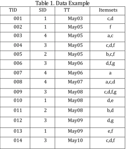
Now let's use the small data shown in Table 1 to explain the detailed behavior of the algorithm mentioned above. In the table, the SID represent the sequence ID and TT columns represent transaction time. The data set is used in the mining of association rules [10] (including frequent itemsets) mining and maximum sequence pattern mining, except that SID and TT are not considered in the example of mining association rules (including frequent itemsets).

Table 1. Data Example

TID SID TT Itemsets 001 1 May03 c,d

002 1 May05 f

003 4 May05 a,c 004 3 May05 c,d,f 005 2 May05 b,c,f 006 3 May06 d,f,g

007 4 May06 a

008 4 May07 a,c,d

009 3 May08 c,d,f,g 010 1 May08 d,e 011 2 May08 b,d 012 3 May09 d,g

013 1 May09 e,f 014 3 May10 c,d,f

From the above, we can see that the Apriori algorithm scans the data set three times in order to obtain frequent itemsets [11]. Below we will see that the AprioriTid algorithm only scans the data set once. The

algorithm uses new datasets

C

1 and C2 when calculating the support for candidate sets in

C

2 and

3

C

_{. Figure 4.2 provides a brief description on how the AprioriTid algorithm finds frequent itemsets from}

these data sets. C2 is obtained by calculating the support for each candidate set in C2, and

C

1 is

obtained directly from the data set. Assuming t001,{{ },{ }}c d C1, the candidate set cd in

C

2 is

added to set

C

t, because the set of itemsets {{c}, {d}} of t contains two 1-items that make up item set cd set. More precisely, cd is added to

C

t because it is a union of two 1-item sets in t. That means transaction

001 supports cd, and there is no other candidate set because transaction 001 cannot support other candidate sets in

C

2. As a result, the support for cd is incremented by 1, and <001,{{cd}}> is also added to

2

C

. Similarly, since transaction 003 supports

2

ac

_C

, <003,{{ac}}> is added to C2. Besides, <002,{{f}}>

in

C

1 will not be added to C2 because transaction 002 does not support any 2-item set. At last, as shown

in Figure 4.2,

C

2 has a total of nine entries, which is smaller than the original dataset. Using the same

method to support the candidate set

3

C

, you can get C3. There is a unique itemset cdf in

C

3. Only 3

items in

C

₂ are reserved in

C

₃. There is a key point that

C

₃ will not be stopped because

4

[12].

Association rules (algorithm 4.2)

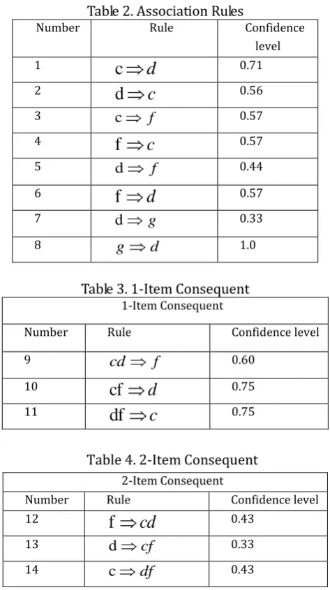
In this section, we use algorithm 4.2 to generate the association rules from the frequent itemsets obtained earlier. Let the algorithm parameter mincof=0.6. At first, let's observe the frequent 2-item sets cd, ef, df, dg. Each frequent itemset only produce two rules. Table 4.2 summarizes these rules and their confidence. 1 and 8 are the association rules for the output of Algorithm 4.2 because they satisfy the constraint of minconf. The ap-genrules procedure is used once for each rule satisfying the constraint. However, there is no output anymore since it no longer generates other rules from the frequent 2- itemset.

Table 2. Association Rules

Number Rule Confidence level

1

_c

_

_d

0.71

2

_d

_

_c

0.56

3 _{c f} 0.57

4

_f

_

_c

0.57

5 _{d f} 0.44

6

_f

_

_d

0.57

7 _d _g 0.33

8 _gd 1.0

Table 3. 1-Item Consequent 1-Item Consequent

Number Rule Confidence level

9 _cd  _f 0.60

10

_cf

_

_d

0.75

11

_df

_

_c

0.75

Table 4. 2-Item Consequent 2-Item Consequent

Number Rule Confidence level

12

_f

_

_cd

0.43

13 _dcf 0.33

14 _cdf 0.43

3.2.

Generate Positive and Negative Association Rules By Frequent Itemsets

This paper think of the positive association rules like the form of

A



B

and the negative association

rules like forms of A B_,  A B_{, and}   A B_. supp A



B



minsFIS _{indicates that}

the association rule describes the relationship between each itemset in a frequent itemset. While





min

supp AB  sFIS _{indicates that the association rule describes the relationship between the}

item set and the itemset in an infrequent itemset. Therefore, the subitems in the itemset need to compare

the conditions supp A

 

minsF SI _and supp

 

B minsF SI _{frequently. Another measure is}

the degree of promotion lift, which is greater than 1 indicating a significant positive correlation between items, while less than 1 indicates a negative correlation between items [14].

Algorithm generates positive and negative association rules through frequent itemsets given:

sup

p A? B





³

mi

ns

- FIS

If

conf(A? B)?minconf & &lift(A? B) > 1

Then

A



B

, a valid positive rule, is greater than the minimum confidence value, and there is a positive

correlation between rule items A and B;

Else if

conf A

(



B

)



min

conf

& &

lift A

(



B

)



1

Then

A



B

is not a valid positive rule, but there may be a negative correlation between rule items A and B, so a negative is generated rule by doing this:

If

conf A

(

  

B

)

min

conf

& &

lift A

(

 

B

)



1

, Then

A

 

B

is a valid negative rule and

there is a positive correlation between rule items A and



B

_; Else if conf( A B)minconf & &lift( A B)1

Then  A B is a valid negative rule and there is a positive correlation between rule items A _and

B;

Else if conf(  A B)minconf & &lift(  A B)1

Then   A B _{is a valid negative rule and there is a positive correlation between rule items}



A

and



B

_[15、16].

4.

Experimental Results and Analysis

Process 1: Find the largest k-term frequent set

a)Apriori algorithm simply scans all transactions. Moreover, each item in the transaction is a member of the set of candidate 1 itemset, calculating the support of each item, such as

itemsets{ }

support

7

=

=0.7

all of transactions

10

a

P({a})



，

b)comparing the support degree of the middle set with the preset minimum support threshold, and retaining the item greater than or equal to the threshold, obtaining a frequent set.

c)Scan all transactions,

L

1and

L

1 are connected to the candidate second itemsets

C

2, and calculate the

support of each item. Such as

itemsets{ , }

support

=

5

=0.5

all of transactions

10

a b

P({a

，

b})



，

. Next is the pruning step.

Since each subset of

C

2(that is

L

1) is a frequent set, no items are removed from

C

2.

d)comparing the support of each set in the pair with a preset minimum support threshold, and retaining items greater than or equal to the threshold, and obtaining two frequent sets.

e)Scan all transactions,

L

2 and

L

1are connected to the candidate 3 sets C3 and calculate the support of

each item, such as

itemsets{ , , }

support

=

3

=0.3

all of transactions

10

a b c

P({a

， ，

b

c})



，

Next is the pruning step. All items connected to

L

2 and

L

1 are: {a,b,c}、{a,b,d}、{a,b, }e 、

{a,c,d}_、{a,c,e}_、{b,c,d}_、{b,c,e}_{. According to the Apriori algorithm, all non-empty subsets of the}

frequent set must also be frequent sets because {b,d}、{b,d} do not contain in the frequent set

L

2 of

the b items. That is, it is not frequent sets and should be eliminated. At last, item set is only

{a,b,c}_and{a,c,e}_in

_C

_3.

According to the Apriori algorithm, all non-empty subsets of the frequent set must also be frequent sets, because (a)(b) does not contain In the frequent set L of the b term, that is, it is not a frequent set, it should be eliminated, and the item set in the last K is only sum of {a,b,c} and {a,c,e} .

f) comparing the support degree of each set in C with a preset minimum support threshold, and retaining items greater than or equal to the threshold, and obtaining three frequent sets

L

3.

g)

L

3 and

L

1 are connected to the candidate set of four

C

4, which is easy to get an empty set after

pruning. Finally, the maximum three frequent sets {a,b,c} and {a,c,e} are obtained.

It can be seen from the above process that

L

1,

L

2, and

L

3are frequent itemsets, and

L

3 is the maximum

frequent item set.

Process 2: Association rules are generated by frequent sets [17]. The confidence formula is calculated as:

( ) _ count( ) ( ) ( | )

( ) _ count( )

Support A B Support A B Confidence A B P A B

Support A Support A

 

   

whereSupport_ count(AB) is the number of transactions that contain the item set

A



B

_;

Support_count(A) _{is the number of transactions that contain item set A. According to this formula, you}

can calculate the confidence of the association rule.

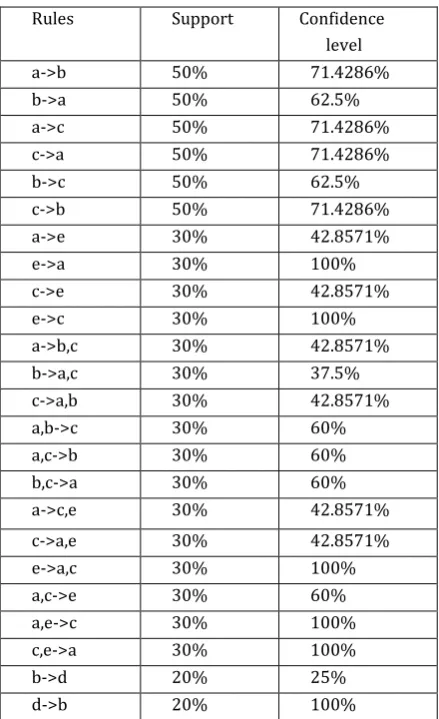
Table 5. Association Rules Rules Support Confidence

level a->b 50% 71.4286% b->a 50% 62.5% a->c 50% 71.4286% c->a 50% 71.4286% b->c 50% 62.5% c->b 50% 71.4286% a->e 30% 42.8571% e->a 30% 100% c->e 30% 42.8571% e->c 30% 100% a->b,c 30% 42.8571% b->a,c 30% 37.5% c->a,b 30% 42.8571% a,b->c 30% 60% a,c->b 30% 60% b,c->a 30% 60% a->c,e 30% 42.8571% c->a,e 30% 42.8571% e->a,c 30% 100% a,c->e 30% 60% a,e->c 30% 100% c,e->a 30% 100% b->d 20% 25% d->b 20% 100%

where we set the minimum confidence to 50%, then the association rule becomes 16 as shown.

Table 6. Association Rules

Rules Support Confidence level a->b 50% 71.4286% b->a 50% 62.5% a->c 50% 71.4286% c->a 50% 71.4286% b->c 50% 62.5% c->b 50% 71.4286% e->a 30% 100% e->c 30% 100% a,b->c 30% 60% a,c->b 30% 60% b,c->a 30% 60% e->a,c 30% 100% a,c->e 30% 60% a,e->c 30% 100% c,e->a 30% 100%

( ) _ count( ) { , } 5

( ) (a | ) 0.714286

( ) _ count( ) { } 7

Support a b Support a b a b Confidence a b P b

Support a Support a a

 

      

( , ) _ count( , ) { , , } 3

( , ) ( | a, ) 0.6

( , ) _ count( , ) { , } 5

Support c a b Support c a b a b c

Confidence a b c P c b

Support a b Support a b a b

 

      

( , ) _ count( , ) { , , } 3

( , ) ( , | ) 1

( ) _ count( ) { } 3

Support a c e Support a c e a c e

Confidence e a c P a c e

Support e Support e e

 

      

5.

Conclusion

This paper proposes an algorithm that effectively generates positive and negative association rules at the same time [19], [20]. It can not only capture the negative correlation between frequent itemsets, but also extract the correlation between infrequent itemsets. The traditional association rule mining algorithm mainly focuses on generating positive correlation rules in frequent itemsets or only uses infrequent [21] itemsets to generate negative association rules. The experimental results show that the proposed method is effective. In the future research, the quality and effectiveness of the generated association rules can be further improved by the algorithm at this paper [22]. The related association rules of intelligence data can improve its efficiency, and thus it provides advantages for how to make decision [23]-[25].

References

[1] Zhigang, W., Chishe, W., & Qingxia, M. (2013). Research on distributed parallel association rules mining algorithm. Computer Applications and Software,30(10), 113-119.

[2] Rubeena, Z., Muhammad, Z. Z., & Naqib, H. (2018). Gender mainstreaming in politics: Perspective of female politicians from Pakistan. Asian Journal of Women's Studies, 24(2).

[3] Weiping, D. (2008). Improvement of association rules mining Apriori algorithm and its application research. Journal of Nantong University(Natural Science Edition), 8(01), 50-53.

[4] Arthur, A., Shaw, N. P., & Gopalan. (2011). Frequent pattern mining of trajectory coordinates using apriori algorithm. International Journal of Computer Applications, 22(9).

[5] Chhagan, C., & Rajoo, P. (2016). Eigenvalue based double threshold spectrum sensing under noise uncertainty for cognitive radio. Optik - International Journal for Light and Electron Optics, 127(15). [6] Zhou, W., & Dan, L. (2016). Research and improvement of Apriori algorithm based on big data

association rules. Library and Information Service, 60(S2), 127-142.

[7] Deepa, D., & Susmita, D. (2017). A novel approach for energy‐efficient resource allocation in double threshold‐based cognitive radio network. International Journal of Communication Systems, 30(9). [8] Kang-Wook, C., Sang-Hyun, H., & Min-Soo, K. (2018). GMiner: A fast GPU-based frequent itemset mining

method for large-scale data. Information Sciences, 439-440.

[9] Zhiyong, Q., & Jinxian, X. (2015). Research on 3D planning assistant decision system. Mapping Geography, 40(04), 90-92.

[10]Sun, S., Antonio, T. O., Ballesteros, N., Dragan, S. P. C., Liu, F., Li, H. F., Zhang, N., Zhang, Y. J., & Wang, Y. (2016). Probabilistic frequent itemset mining algorithm over uncertain databases with sampling. Frontiers in Artificial Intelligence and Applications, 293.

[11]Ruizhi, T., Songyan, K., & Xinghong, L. (2015). Research on position sensorless control of switched reluctance motor based on double threshold hysteresis algorithm. Micro-motor, 48(10), 59-62.

[12]Mengli, R., & Lei, W. (2018). Association rule mining method based on double threshold Apriori algorithm and infrequent itemsets. Computer Applications, (12). Retrieved July 29, 2018, from http://kns.cnki.net/kcms/detail/51.1196.TP.20180427.1652.002.html

[13]Baohua, L., & Min, C. (2010). Improvement of mining method of positive and negative association rules and its application. Computer Engineering, 36(16), 44-46.

Harbin University of Science and Technology.

[15]Yun, L., Jie X., Yunhao Y., & Ling, C. (2017). A new closed frequent itemset mining algorithm based on GPU and improved vertical structure. Concurrency and Computation: Practice and Experience, 29(6). [16]Hongtao, Q., Shenwu, K., Shenyu, F., & Min, Z. (2018). Intelligent integrated decision mobile operator

terminal ideas (to be continued) — A new model for sharing power big data and transparent computing based on the power service command platform. Rural Electrician, 26(06), 9-10.

[17]Tao, G., & Daiyuan, Z. (2011). Research and application of Apriori algorithm based on association rules data mining. Computer Technology and Development, 21(06), 101-107.

[18]Fengxiao, S., Shihong, N., & Chuan, X. (2013). A matrix-based Apriori improved algorithm. Computer Simulation,30(08), 245-249.

[19]Rui, Q., & Tianjiao, Z. (2017). Apriori improved algorithm based on matrix compression. Computer Engineering and Design, 38(08), 2127-2131.

[20]Min, L., & Sha, L. (2017). A weighted Apriori improved algorithm. Journal of Xi'an University of Posts and Telecommunications, 22(04), 95-100.

[21]Wei, W. (2012). Research and Improvement of Apriori Algorithm in Association Rules. Ocean University of China.

[22]Pankaj, V., & Brahmjit, S. (2016). Throughput maximization by alternative use of single and double thresholds based on energy detection method. Optik - International Journal for Light and Electron Optics, 127(4).

[23]Ning, D. (2016). Research and improvement of Apriori algorithm based on data mining. Automation and Instrumentation, (09), 232-234.

[24]Xiyu, L., Yuzhen, Z., Minghe, S., & Stefan, B. (2017). An improved Apriori algorithm based on an evolution-communication tissue-like p system with promoters and inhibitors. Discrete Dynamics in Nature and Society.

[25]Zhichun, W. (2015). An improved mining association rule Apriori algorithm. Computer Knowledge and Technology,11(34), 4-17.

ZhangJie was born in Anhwui, China in 1995. He is pursuing his M.Sc on information and communication engineering major at graduate school of air force engineering university. His research interests combat multi-agent based on a deep learning and combat level of tactical air defense and antimissile.

Wang Gang received his M.Sc degree in Air Force Engineering University and received Ph.D from Air Missile Defense College of Air Force Engineering University. Currently, he is a professor at Air Force Engineering University. His research interests machine learning, information fusion and command and control system.

Aut