Parallel Processor Design and Implementation
for Molecular Dynamics Simulations on a
FPGA-Based Supercomputer
Server Kasap
Department of Electronical and Electrical Engineering, European University of Lefke, Mersin-10, Turkey Email: [email protected]
Khaled Benkrid
School of Engineering, University of Edinburgh, King’s Buildings, Mayfield Road, Edinburgh, EH9 3JL, UK Email: [email protected]
Abstract—The design and implementation of an FPGA core that parallelises all the necessary operations to compute the non-bonded interactions in a MD simulation with the purpose of accelarating the LAMMPS MD software is presented in this paper. Our MD processor core comprised of 4 identical pipelines working independently in parallel to evaluate the non-bonded potentials, forces and virials was implemented on the nodes of a FPGA-based supercomputer named Maxwell. Implementing our FPGA core on multiple nodes of Maxwell allowed us to produce a special-purpose parallel machine for the hardware acceleration of MD simulations. The timing performance figures of this machine for the pairwise LJ and short-range Coulombic (via PPPM) interaction computations in the MD simulations of the solvated Rhodopsin protein systems with various numbers of atom show performance gains over the pure software implementation by factors of up to 13 on two nodes of the Maxwell machine. Furthermore, our MD machine is highly scalable, yielding higher computational power with the additional Maxwell nodes. To our knowledge, this is the first attempt to port an existing production-grade MD software to a FPGA-based parallel computer.
Index Terms—High Performance Reconfigurable Computing, Molecular Dynamics, Field-Programmable Gate Array (FPGA).
I. INTRODUCTION
Computer simulations are carried out to understand the properties of assemblies of molecules in terms of their structure and the microscopic interactions between them [1]. They act as a bridge between microscopic length and time scales and the macroscopic world of the laboratory, serving as a complement to conventional experiments. Carrying out simulations on computers that are either difficult or impossible in the labarotory enables us to learn something new, something that can not be found out in other ways.
There are two main families of simulation techniques: Molecular Dynamics (MD) and Monte Carlo (MC)-based simulations. There are also several hybrid techniques which combine features from both. MD is a deterministic simulation technique whereas simulation results from MC simulations are stochastic. Furthermore, MD can provide the dynamic properties of the simulated system as well as the static properties, as opposed to MC.
In MD, the time evolution of a set of interacting atoms modelled with classical mechanics is followed by inte-grating their Newtonian equations of motion. MD simula-tions of biomolecules provide a molecular picture of the structure and behaviour of biological systems such as enzymes, proteins, DNA strands and membranes. This allows scientists to advance their understanding of bio-logically important molecules. The MD method has ap-plications in the fields of protein engineering [2], drug design [3], [4] and refinements of structures based on X-ray [5] and NMR experiments [6].
However, biological systems of interest have sizes ranging from a few tens of thousands to millions of atoms. Performing MD simulation of a biological process, such as protein folding, for a reasonable physical time requires enormous amounts of computational effort and may take years to complete on conventional comput-ers. Therefore, it is mandatory to utilize faster computing platforms.
Acceleration of MD simulation using special-purpose computers has started to attract interest as a result [17]. Field Programmable Gate Arrays (FPGAs) in particular have recently been proposed as a viable alternative im-plementation platform for MD simulation due to their flexible computing and memory architecture which gives them ASIC-like performance with the added programma-bility feature. Therefore, we chose FPGAs over ASICs as they offer reprogrammability, shorter development times and lower nonrecurring engineering (NRE) costs.
There are several MD simulation software tools. How-ever, they can spend a very high percentage of the total computation time in calculating the non-bonded interac-tions among particles because the computational com-Corresponding author: Server Kasap [email protected]
plexity of the evaluation of non-bonded potentials or forces is quadratic. Therefore, we can accelerate MD simulation by porting the calculation of the non-bonded interactions from software to FPGAs since non-bonded interactions lend themselves to be easily calculated in parallel. On the other hand, the remaining MD calcula-tion, which is complex but only consumes a very limited percentage of the total computation time, can be left to software running on a host computer. Our ultimate goal is to design and implement a MD simulation sytem that will allow scientists to simulate a biomolecular system within a reasonable time frame and obtain useful information of a biological system.
The design and implementation of an FPGA core that parallelises all the necessary operations to compute the non-bonded interactions in the Large-scale Atomic/Molecular Massively Parallel Simulation (LAMMPS) software tool is explained in this paper. Our MD processor core is comprised of 4 identical pipelines working independently in parallel to evaluate the non-bonded potentials, forces and virials acting on a particle from all of the other particles in the simulated molecular system. A real hardware implementation of the designed core was achieved on the nodes of a FPGA-based super-computer, called Maxwell, which consists of 64 Virtex-4 FPGA chips. Implementing our FPGA core on multiple nodes of Maxwell allowed us to produce a special-purpose parallel machine for the hardware acceleration of MD simulations. This machine is highly scalable, yield-ing higher computational power with the additional Maxwell nodes.
To our knowledge, our work is one of few which at-tempt to port an existing production-grade MD software to FPGAs rather than an unoptimized textbook MD code. As a novelty, our work is scaled up to many nodes on a FPGA-based supercomputer. We are also calculating the potential and virial values in contrast to similar attempts. Furthermore, our paper presents the detailed design for the non-bonded interaction computations unlike many other papers.
The remainder of this paper will first present essential background information on MD simulation and then dis-cuss related prior works in the literature. Subsequently, LAMMPS MD simulation software will be introduced. After that, our implementation platform (the Maxwell FPGA-based supercomputer) will be illustrated and the general system architecture will be explained. Further-more, the design and implementation of our FPGA core for computing the non-bonded interactions in a MD simu-lation will be elaborated. Following this, implementation results are presented and then evaluated comparatively with equivalent pure software implementations. Finally, conclusions are laid out with plans for future work.
II. MOLECULAR DYNAMICS SIMULATION Molecular Dynamics is commonly used for the simula-tion of the structural, thermodynamic and transport prop-erties of large biological systems on a diverse range of timescales. In MD simulations, atoms in the system are treated as classical particles and are subject to covalent
bond, Van der Waals and Coulomb forces from other par-ticles. During a time-step of the MD simulation, forces are computed and accumulated on each atom due to its interaction with other atoms, and positions and velocities of atoms are updated by integrating the Newtonian equa-tions of motion.
A. Molecular Interactions
In MD simulations of biological systems, the potential for a particle i, Φi , is modelled as follows:
(1)
where rji is a vector from the particle j to i and qi is the
charge of the particle i. The first term ΦiB is the bonded
potential due to interactions within the topology of the molecules and is expressed as:
(2)
Bonded potential is written here as sums over sim-ple harmonic 2-body (bond), 3-body (angle) and 4-body (dihedral) interactions although other potential models could also be used. On the other hand, the last 2 terms in (1) are the non-bonded potential due to interactions be-tween all pairs of atoms in the system. Note that the forces exerted on the particle i, fi, are obtained by taking
the gradient of (1) with respect to the position of the par-ticle.
The second term in (1), which describes van der Walls interaction, is the Lennard-Jones (LJ) potential characte-rized by a length parameter ab and an energy parameter
ab where a and b denote the two atom types of particles.
If we take the gradient of this potential, an LJ force fiLJ
can be expressed as:
(3)
The third term on the right hand side of (1) is the Cou-lombic (C) potential, and the corresponding CouCou-lombic force fiC is expressed as:
(4)
The computational complexity of evaluating ΦiB is
O(1) since only few particles are covalently bonded to the ith particle. However, the computation time to evaluate
prime target for the design of our MD core. Note that our MD processor core will be able to deal with an arbitrary potential or force function although only the LJ and Cou-lombic interactions are mentioned in this section.
B. Cutoff Convention
The simplest method for reducing the computation time is the cutoff convention. Contributions from par-ticles outside a certain cutoff radius rc are ignored in this
method and hence, the time complexity is reduced to O(N). For instance, since LJ force and potential decrease rapidly with increasing distance (refer to (3)), the sum over j can be truncated within the determined cutoff dis-tance so that only a few neighbours of atom i contribute rather than all N. This does not affect the results in most cases provided that the particles are well separated with respect to an appropriate value of rc.
In contrast, the Coulombic interaction is long-range which means it decreases slowly with an increase of dis-tance (refer to (4)). Hence, evaluating Coulombic force as a truncated sum over neighbours rather than as a full sum introduces large inaccuracies [7]. On the other hand, ap-plying the latter method is problematic in periodic sys-tems (briefly mentioned in subsection II.D below). Con-sequently, other methods are often used for the evaluation of Coulombic force and potential. One of these methods, namely the Ewald method, is discussed in subsection II.E and the one used by the LAMMPS software is explained in subsection IV.A.
C. Virials
Virials represent the effect of mutual interaction of par-ticles on the pressure in the system. The virial vion the
particle i can be calculated with the following equation where T denotes the transpose of the vector:
(5)
Note that the time complexity of this operation for all particles is O(N2) since it is O(N) for each particle. Our
MD processor incorporates the computation of all com-ponents of each virial.
D. Periodic Boundary Conditions
MD simulations are generally performed under period-ic boundary conditions where the original simulation cell is deemed to be surrounded by its 26 image cells [1]. Then, minimum image convention should be adopted in the calculations of pairwise interactions. This means that a force exerted on the particle i from the particle j is only to be calculated for the real particle j or nearest image of it to the particle i.
E. Ewald Method
In the cases where periodic boundary conditions apply and hence, electrically charged particles exist periodical-ly, Coulombic forces can be calculated precisely by the Ewald method [8]. Force fiCis split into the sum of two
rapidly converging series in the Ewald method as fol-lows:
(6)
where fir is the real space sum and fim is the reciprocal
space sum. The real space sum is given in (7) where the positive parameter is taken to be an appropriate value so that the fir converges rapidly.
(7)
In (7), erfc is the complementary error function which is defined as:
(8)
Our MD processor can evaluate fir according to (7)
whose computation time is O(N2) for all particles since it
is O(N) for each particle. On the other hand, the computa-tion of fimis left to the software running on a host
proces-sor in our implementation. F. Time Integration
There are various kinds of integrators to integrate Newtonian equations of motion, such as Verlet algorithm [9], Beeman algorithm [10], and multiple time-step rithms [11]. One of the simplest and most popular algo-rithms for the time integration of the positions and veloci-ties of particles is the Verlet algorithm which is expressed as the following two equations:
(9)
(10) where r (t), v (t) and a(t) are the position, velocity and acceleration vectors of a particle at time t, respectively and δt denotes the chosen size of each time-step. Note that the acceleration of a particle at a time-step is com-puted by the Newton’s second law of motion:
(11)
III. PRIOR WORK
research topic is to speed-up the most computationally intensive portion of the MD simulation computation, namely the non-bonded interactions.
MD-GRAPE [17], [18] is one of the most prominent hardware acceleration systems for MD simulations. It uses a fourth order polynomial with 1024 piece to ap-proximate the calculation of the force or potential where the coefficients determine which force or potential is cal-culated. MD-GRAPE which has a peak speed of 4.2 Gflops only accelerates the computation of the force and potential while leaving the rest of the MD simulation to a host processor. MD engine [19] was also a special-purpose computer for MD simulation which had system architecture similar to that of the MD-GRAPE system, where the host computer communicates with the special-purpose parallel machine that computes the non-bonded interactions.The MD engine system consists of 76 indi-vidual processors named MODEL each of which calcu-lates both the Lennard-Jones and Coulombic interactions. The system can perform the simulation 50 times faster than an equivalent software implementation running on a Sun Ultra-2 200 MHz machine.
All of the aforementioned special-purpose hardware platforms for MD simulation were implemented using ASIC technology. However, hardware development in this way can take up several years before the application is fully implemented. On the other hand, recent advances have made FPGAs a viable platform for accelerating MD simulations with substantial performance gains. There-fore, recent academic research has attempted to imple-ment special-purpose computers for MD simulation using FPGAs.Prior reserach on FPGA-based MD simulations have concentrated on accelerating different parts of the MD simulation. One of them mapped the position and velocity update to FPGA [20] while most of them com-puted LJ and Coulombic interactions of each time-step on FPGA [21], [22], [23], [24], [46], [47]. On the other hand, only few ones moved all tasks in MD simulation onto FPGA [25], [26].
However, only few of these efforts are concerned with the problem of accelerating an existing MD simulation software [24], [47]. Most of them just implement simple textbook algorithms without any optimization. Hence, these attempts to accelerate MD simulation do not have much, if at all, practical benefits. On the contrary, we targeted a production-grade molecular dynamics code that is highly optimized to run on parallel systems and is frequently used by the scientific community. Therefore, our design is certainly much more capable of accelerating real MD simulations, compared to many others, for the purpose of allowing scientists to simulate biomolecular systems in reasonable times. Furthermore, our work is the first reported FPGA-based supercomputer acceleration of MD simulations.
IV. LAMMPS MD SIMULATION SOFTWARE LAMMPS is a classical molecular dynamics code writ-ten in C++, which stands for Large-scale Atom-ic/Molecular Massively Parallel Simulator [27]. It was developed at Sandia National Laboratories under the US
department of Energy as a freely-available, open-source code, distributed under the terms of the GNU public li-cense.
LAMMPS runs on single-processor machine although it was designed to run most efficiently on parallel com-puters supporting the MPI message-passing library, for instance on distributed- or shared-memory parallel ma-chines and Beowulf-style clusters. LAMMPS can model atomic, polymeric, biological, metallic, granular and coarse-grained systems with only a few particles up to millions or billions using a variety of force fields and boundary conditions. However, it was designed to be easily modified or extended with new capabilities, such as new force fields, atom types or boundary conditions.
LAMMPS partitions the simulation domain into small 3D subdomains with spatial decomposition techniques on parallel machines. Each subdomain is assigned to a pro-cessor, and processors communicate and store ghost atom information for atoms that border their subdomain. By subdividing the physical volume among processors, most computations become local and communication is mini-mized so that optimal N/P scaling of the overall calcula-tion can be achieved on P processors. Hence, the spatial-decomposition method is clearly the best algorithmic choice in comparison with atom decomposition and force decomposition methods both of which do not scale well to large numbers of processors. Note that systems with uniform particle density are most efficiently simulated by LAMMPS on parallel machines.
In the simplest sense, LAMMPS integrates Newton’s equation of motion for particles interacting via short- or long-range forces. It utilizes neighbour lists to keep track of the nearby particles for each particle so that the short-range, non-bonded potentials and forces for all particles are computed efficiently using cutoff convention (see subsection II.B) with time complexity of O(N). As atoms move, these lists are reformed at every few time-steps, taking into consideration both owned and ghost atoms, with the utilization of a certain threshold radius (i.e. rc +
an offset) to determine the neighbouring particles for a particle.
There are several ways to enable the quick calculation of the Coulombic interactions by avoiding the all-pairs O(N2) computation. Approximate techniques include multipole methods [28], [29] scaling as N, Ewald summa-tion (see subsecsumma-tion II.E) scaling as N3/2 and
particle-particle particle-particle-mesh method (PPPM) [30] scaling as N log (N)1/2. PPPM which is a variant of particle-mesh Ewald (PME) method [31] is the method used by LAMMPS for the Coulombic computations due to its higher computational efficiency relative to other methods, particularly in parallel setting, as described in subsection IV.A.
Papers [32], [33] elaborate on the technical details of the algorithms used in LAMMPS.
A. PPPM Method
the point charge Coulombic term in (1) with an equiva-lent expression for extended charges centered on the orig-inal atomic positions. Hence, Coulombic potential is now expressed as follows:
(12)
where is the Gaussian density that represents an extended charge and is given as follows:
(13)
The first term in (12) is the usual Coulombic potential multiplied by a complementary error function which forces it to go to nearly zero at a user-specified cutoff distance rc,where G is determined by the accuracy
crite-rion. Thus, this term is the short-range portion of the Coulombic interaction and is computed in LAMMPS at the same time as van der Waals interactions as a sum over nearby particles utilising neighbour lists. On the other hand, the second term in (12) is the Coulombic potential due to the interaction of the extended charges whereas the last term is a constant.
V. THE MAXWELL SUPERCOMPUTER
Maxwell [35] is an FPGA based supercomputer devel-oped by the FPGA High Performance Computing Al-liance (FHPCA) in Scotland [36] to run computationally demanding applications on an array of FPGAs at low energy budgets. Its physical architecture, logical structure and software environment are briefly discussed in subsec-tions V.A, V.B and V.C, respectively.
A. Physical Architecture
Maxwell comprises two 19-inch racks and five IBM blade centres, four of which have seven IBM Intel Xeon blades and the fifth has four (32 blades in total). The blades are booted over the network from the head node (Dell server). Furthermore, each blade is a diskless 2.8 GHz Xeon with 1 Gbyte memory which hosts two Xilinx Virtex-4 FPGAs through a PCI-X expansion module. Thus, Maxwell comprises 64 FPGAs having 512 or 1024 MB off-chip memory and four Multi-Gigabit Transceiv-ers (MGTs) which can run at 2.5 Gb/s. Furthermore, the FPGAs are mounted on 2 different types of plug-in PCI card, namely Alpha Data ADM-XRC-4FX [37] and Nal-latech HR101 [38]. Both types of card connect to the Xeon on a particular blade using a PCI/PCI-X bridge which is capable of 32 bit, 133 MHz operation in PCI-X mode, giving a peak bandwidth of 532 MB/s.
Maxwell has three independent networks for CPU-CPU, CPU-FPGA, and FPGA-FPGA communications. The blade CPUs are networked over Gigabit Ethernet through a single 48-way Netgear switch with 40 Gb/s throughput. Thus, CPUs have an all-to-all connectivity. The FPGA network consists of point-to-point links
be-tween the MGT connectors of adjacent FPGAs. Since each FPGA has 4 MGTs, the 64 FPGAs are connected together in a two-dimensional 8 x 8 torus. Finally, FPGAs and CPUs can communicate with each other over the PCI bus as mentioned above.
B. Logical Structure
Logically, Maxwell can be regarded as a collection of 64 nodes, where a node is defined as a software process running on a host CPU together with some FPGA accele-ration hardware. In the typical case of 64 nodes configu-ration, each blade CPU hosts two software processes each of which manages one of the two FPGAs on the blade during runtime.
C. Software Environment
The software environment of Maxwell comprises Li-nux distribution CentOS, standard GNU/LiLi-nux tools, Sun Grid Engine (SGE) as the batch scheduling system, Mes-sage Passing Interface (MPI) [41] for inter-process com-munication and most importantly the FHPCA Parallel Toolkit (PTK) [39] that forms a bridge from the applica-tion process to the FPGA process. Essentially, the PTK is a set of practices and infrastructure written mostly in C++ that aims to address acceleration issues such as associat-ing processes with FPGA resources, associatassociat-ing FPGAs with bitstreams, managing contention for FPGA re-sources within a process and managing code dependen-cies to facilitate re-use.
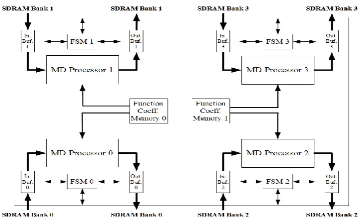
VI. SYSTEM ARCHITECTURE
Figure 2. Sytem connection diagram of our special-purpose parallel machine for Molecular Dynamics simulations Figure 1. Basic structure of our special-purpose parallel machine for
Molecular Dynamics simulations.
The total potential energy and pressure in the simu-lated system at the current time-step are also calcusimu-lated by accumulating these potential and virial values, respec-tively. Note that a new C++ class was written for the LAMMPS software using the FHPCA Parallel Toolkit (PTK) to be able to co-operate with the reconfigurable hardware for MD simulations in the way explained above. Another important point is that all transfers be-tween host CPU and reconfigurable hardware are done with Direct Memory Access (DMA) method.
Fig. 2 shows the system connection diagram of our spe-cial-purpose parallel machine for MD simulations. Two processes of LAMMPS software run on each Intel Xeon CPU while an instance of our MD processor core resides in each user FPGA. Actually, a software process running on a host CPU and a hardware core in a user FPGA form a Maxwell node as described in subsection V.B. The number of utilized Maxwell nodes where LAMMPS processes communicate with each other by MPI can be easily confi-gured as desired.
Each Xeon CPU on PCI-X bus connects to two user FPGAs through bridge/control FPGAs mediating commu-nication between the 32-bit wide PCI-X bus operating at 133 MHz and the 32-bit wide local buses of the user FPGAs operating at 80 MHz, as shown in fig. 2. Further-more, user FPGAs in our MD machine are of Xilinx Vir-tex-4 FX-100 type whereas smaller FPGAs bridging PCI-X and local buses are of PCI-Xilinx Virtex-4 LPCI-X25 type. On the other hand, four 256 MB DDR2 SDRAMs are connected to each user FPGA. The physical width and depth of the SDRAMs are 32 bits and 64M words, respectively while the logical width of the SDRAMs is 128 bits. Note that the MD processor core in a user FPGA runs at 150 MHz al-though the logic interfacing the user FPGA to the local bus it is connected to runs at 80 MHz.
Figure 3. Sytem connection diagram of our special-purpose parallel machine for Molecular Dynamics simulations
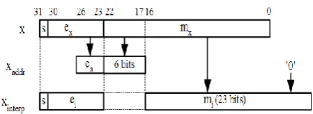
Figure 4. (a) Internal format of the numbers used in our design (b) Layout of a memory portion in the first region of a SDRAM bank stor-ing the coordinates and electric charge of a particle i (c) Layout of another memory portion in the first region of a SDRAM bank storing the coordinates and electric charge of a j particle as well as the interac-tion parameters and the cutoff distances for the particular pair of i and j particles (d) Layout of a memory portion in the second region of a SDRAM bank storing the force, potential and virial values computed for the specific pair of i and j particles.
VII. DESIGN OF MOLECULAR DYNAMICS PROCESSOR In our design, internal format of the numbers used is the IEEE standard single precision (i.e. 32-bit wide) float-ing-point as shown in fig. 4 (a). All data are handled in this format. Hence, single precision floating-point arith-metic units are utilized throughout our MD processor. Several pipelined floating-point multipliers and ad-ders/subtractors obtained from [42] are incorporated in our design whose operation latencies are 4 and 6 clock cycles, respectively, as explained in [43]. These arithmet-ic units do not support denormalized numbers and NaN (“not a number”) to minimize the required hardware re-sources and realize high operation speed by simplifying the circuitry.
SDRAM banks in our MD machine were partitioned into two regions. The first region of a SDRAM bank was allocated to data transfers from host CPU while the second region was allocated to data transfers from the designated MD processor on a user FPGA, as mentioned in section VI. Fig. 4 (b) shows the layout of a memory portion in the first region of a SDRAM bank storing the coordinates ri = (rx, ry, rz) and electric charge qi of a
par-ticle i whereas fig. 4 (c) shows the layout of another memory portion in the first region of a SDRAM bank storing the coordinates rj = (rx, ry, rz) and electric charge
qj of a j particle, as well as the interaction parameters εij,
ζ-2
ij and the cutoff distances for both Lennard-Jones rLJij
and Coulombic rC
ij interactions, all pertaining to the
par-ticular pair of i and j particles. Since the logical width of the memory banks is 128 bits, the layouts in fig. 4 (b) and (c) occupy the space of 1 and 2 logical words, respective-ly. Furthermore, the layout of a memory portion in the second region of a SDRAM bank storing the force fij =
(fx, fy, fz), Lennard-Jones potential eLJij, Coulombic
poten-tial eC
ij and virial vij = (vx2, vy2, vz2, vxy, vxz, vyz) values
computed for the specific pair of i and j particles is dis-played in fig. 4 (d) which takes up the space of 3 logical words in a memory bank.
Figure 5. Functional block diagram of a Molecular Dynamics processor
the order presented. MD processor whose operating fre-quency is 150 MHz calculates the non-bonded interac-tions in the simulated molecular system as stated above. The detailed architectures and operations of the three functional units in the MD processor will be described in subsections VII.A, VII.B and VII.C, respectively.
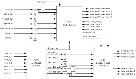
A. MD Distance Squared Unit
Fig. 6 shows a simplified pipeline architecture of the first functional unit in our MD processor, MD Squared Distance unit whose primary duty is to calculate the squared distance between an i particle and the j particles in the neighbour list of that i particle. When a MD processor is triggered by the host CPU, it begins to transfer simulation data of i and j particles into its input buffer (see fig. 3) from the first region of its associated SDRAM bank. Input buffers in our design make use of double buffering so as to enhance the efficiency of the data transfers from a memory bank and hence, increase the operation speed of the MD processors. Note that each of these double buffers has a width of 256 bits, so two logical words are transferred one by one from a SDRAM bank to make up one word of the buffer.
When an input buffer is completely full with data, the MD Squared Distance unit starts to read one word from the buffer every four clock cycles. If it is detected that the read word contains the coordinates and electric charge of an i particle, those coordinates are registered separately in the unit (not shown in fig. 6) whereas the charge value is shifted towards the MD Calculation unit in a register array as shown in fig. 5. On the other hand, if the read word contains data related to a j particle, coordinate values in that word are registered and then pushed into the pipeline with the valid_in signal asserted for four clock cycles, while the rest of the data in the word (see fig. 4 (c)) are seperately shifted towards the MD
Calculation unit in five register arrays.
When the coordinate values of a j particle enters the pipeline, three floating-point subtractors are used to com-pute the coordinate differences between the registered i particle and that j particle in three dimensions, dij = (dx,
dy, dz), independently in parallel. These coordinate
differ-ences are shifted separately towards the end of the unit in three register arrays to be passed to the MD Force/Virial/Potential unit. Furthermore, two floating-point multipliers compute the two squared coordinate differences in x and y dimensions, dx2, dy2, and the
squared coordinate difference in z dimension, dz2, in
dif-ferent clock cycles through the use of the three multiplex-ers whose control signal values are determined depending on the value of the 2-bit counter valid_cnt which incre-ments by one with the high value of the delayed valid_in signal as shown in fig. 6. Table I shows how the values of the control signals for the multiplexers vary depending on the value of the counter valid_cnt. With these control signal values, two floating-point multipliers also compute the following products of the coordinate differences: dxdy,
dxdz and dydz in addition to dx2, dy2 and dz2 in an order
dictated by the multiplexers. Moreover, all of these coor-dinate difference products are shifted towards the end of the unit in two register arrays to be passed to the MD Force/Virial/ Potential unit for further computations.
TABLEI.
CONTROL SIGNAL VALUES FOR THE THREE MULTIPLEXERS IN THE MD DISTANCE SQUARED UNIT
valid_cnt 0 1 2 3
c_mux_0 0 1 2 X
c_mux_1 0 0 1 X
Figure 6. Simplified pipeline architecture of the MD Distance Squared unit
Finally, the first floating-point adder in the unit com-putes the sum of the squared coordinate differences in x and y dimensions, dx2 + dy2, while the second
floating-point adder adds the squared coordinate difference in z dimension, dz2, to this sum to calculate the squared
dis-tance, r2
ij = dx2 + dy2 + dz2, between a pair of i and j
par-ticles. Furthermore, this value is passed to the MD Calcu-lation unit to evaluate several functions of distance. Note that the pipeline latency of the MD Squared Distance unit is 22 clock cycles.
B. MD Calculation Unit
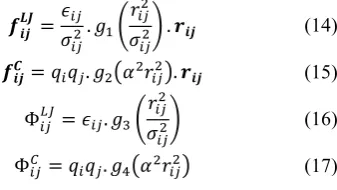
Fig. 7 shows the simplified pipeline architecture of the second and largest functional unit in our MD processor, MD Calculation unit whose primary duty is to calculate and separately multiply the first two terms in (14) and (15), and both terms in (16) and (17). The multiplied terms are then passed to the MD Force/Virial/Potential unit for the computations of the pairwise forces, virials and potentials due to both Lennard-Jones and Coulombic interactions between an i particle and the j particles in the neighbour list of that i particle. Note that only the short-range portion of the Coulombic interactions is computed in our MD processor.
(14)
(15)
(16)
(17)
When the squared distance between a pair of i and j particles is passed to the MD Calculate unit by the MD Squared Distance unit, this value is registered to be valid for four clock cycles with the asserted valid_in signal.
Then, two floating-point comparators in the unit compare the registered squared distance with the specified cutoff distances for the Lennard-Jones and Coulombic interac-tions, respectively. If the squared distance happens to be bigger than the cutoff distance for any interaction, then the forces, virials and potentials due to that interaction are set to be zero for the particular pair of i and j particles. Furthermore, utilizing the values shifted into the unit as shown in fig. 5, the first terms in (14), (15), (16) and (17) are computed to be available at the output of the multip-lexer mux_3 in four consecutive clock cycles through the use of the floating-point multiplier mult_0 and the two multiplexers, mux_0 and mux_1, shown in fig. 7. Control signal values of the mentioned multiplexers and the mul-tiplexer mux_2 are determined depending on the value of the 2-bit counter valid_cnt as shown in Table II.
TABLEII.
CONTROL SIGNAL VALUES FOR THE FOUR MULTIPLEXERS IN THE MD CALCULATOR UNIT
valid_cnt 0 1 2 3
c_mux_0 0 1 0 1
c_mux_1 0 1 0 1
c_mux_2 0 1 0 1
c_mux_3 0 0 1 0
On the other hand, the floating-point multiplier mult_1 computes the arguments of the functions g1(x), g2(x),
g3(x) and g4(x), which are in the second terms of (14),
Figure 7. Simplified pipeline architecture of the MD Calculation unit
Figure 8. The operation required for the polynomial interpolation with a look-up table to evaluate the functions g1(x), g2(x), g3(x) and g4(x).
(18)
(19)
(20)
(21)
Finally, the floating-point multiplier mult_2 multiplies the delayed output of the multiplexer mux_3 and the out-put of the MD Function Evaluator unit, and hence gets the first two terms in (14) and (15) and both terms in (16) and (17) multiplied in 4 consecutive clock cycles for a pair of i and j particles. These results are then sent to the MD Force/Virial/Potential unit with the asserted va-lid_md_calc signal for further processing. Note that the pipeline latency of the MD Calculator unit is 40 clock cycles.
1) MD Function Evaluation Unit
Fig. 9 shows the simplified pipeline architecture of a functional unit in our MD Calculation unit, namely MD Function Evaluation unit which evaluates the functions g1(x), g2(x), g3(x) and g4(x), which are expressed
respec-tively in (18), (19), (20) and (21), consecurespec-tively in four clock cycles using the piecewise (1024 pieces) third-order polynomial interpolation. When the argument x enters the unit with the asserted valid_in signal, it is decomposed into two numbers, xaddr and xinterp, as shown in fig. 8.
The floating-point number xaddr represents the argu-ment x in the range of [2-5, 211) using 10 bits, 4 for the exponent and 6 for the mantissa. The latter is the copy of the most significant bits of the mantissa of x, namely mx. The unit calculates the value of ea ex
addr
x
x 2 , where ea and ex are the exponents of xaddr and x, respectively, and normalizes it in a 32-bit floating-point number xinterp.
Actually, the exponent of xinterp, namely ei, is equal to ex-7-n, where n is the number of leading zeros in the 17 least significant bits of x. Then, a function g(x) can be approx-imated with xinterp as follows, where c3, c2, c1 and c0 are
the coefficients of the piecewise polynomial interpola-tion:
(22)
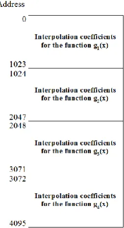
A set of the quadruples of the coefficients (i.e. a look-up table) is stored in the two identical Function Coeffi-cients memories shown in fig. 3. Note that each Function Coefficients memory serves two separate MD processors with its dual port. These memories are comprised of four sub-memories storing one of the four piecewise interpola-tion coefficients (i.e. c3, c2, c1, c0) for four functions (i.e.
g1(x), g2(x), g3(x), g4(x)) in four separate regions. Each
sub-memory is a 4096 x 32 bits Block RAM with an ad-dress width of 12 bits. The layout of a sub-memory in the Function Coefficients memory is shown in fig. 10.
Figure 9. Simplified pipeline architecture of the MD Function Evaluator unit
Figure 10. The layout of a sub-memory in the Function Coefficients memory storing one of the four piecewise interpolation coefficients for the functions g1(x), g2(x), g3(x) and g4(x) in four separate regions.
the four addresses, coming respectively from the four 2-bit counters in the unit, are used to select one out of four tables (functions) stored in the sub-memories. With this configuration, MD Function Evaluation unit evaluates the functions g1(x), g2(x), g3(x) and g4(x) for a pair of i and j
particles in four consecutive clock cycles with a latency of 31 clock cycles.
C. MD Force/Virial/Potential Unit
Fig. 11 shows the simplified pipeline architecture of the third and final functional unit in our MD processor, MD Force/Virial/Potential unit whose primary duty is to compute the pairwise virials and forces acting on an i particle due to both Lennard-Jones and Coulombic inte-ractions with the j particles in the neighbour list of that i particle. In four consecutive clock cycles, the multiplied first two terms of (14), (15), (16) and (17) are pushed one by one into the unit by the MD Calculation unit with the valid_in signal asserted for four clock cycles. Obviously, these four products pertain to the LJ force, Coulombic force, LJ potential and Coulombic potential for a pair of i and j particles, respectively.
The first and second values entering the unit are regis-tered separately in the first two clock cycles under the control of the 2-bit counter valid_cnt, which increments by the high value of the valid_in signal, as shown in fig. 11. These registered values are then added up by the floating-point adder in the unit and the result is passed to the three floating-point multipliers. On the other hand, the third and fourth values are buffered respectively in the synchronous write, asynchronous read buffers fifo_elj and fifo_ecb in the third and fourth clock cycles under the control of the counter valid_cnt. These bufferings last until the end of the operation of these multipliers, as will be explained later.
Furthermore, the three floating-point multipliers com-pute all three components of the total pairwise force fij
(i.e. fx, fy, fz) and six components of the pairwise virial vij
(i.e. vx2, vy2, vy2, vxy, vxz, vyz) in parallel in three
consecu-tive clock cycles by multiplying the output of the float-ing-point adder with the coordinate differences (i.e. dx, dy,
dz) and the coordinate difference products (i.e. dx2, dy2,
dz2, dxdy, dxdz, dydz) ,which are shifted into the pipeline
Figure 11. Simplified pipeline architecture of the MD Force/Virial/Potential unit
is multiplied by the coordinate differences, dx, dy and dz,
to calculate the components of the total pairwise force, fx,
fy, fz, whereas the adder output is multiplied by the
fol-lowing coordinate difference products: dx2, dy2 and dz2 to
compute the following three components of the pairwise virial: vx2, vy2 and vy2 in the second clock cycle. Finally,
in the third clock cycle, the following coordinate differ-ence products: dxdy, dxdz and dydz are multiplied by the
output of the adder to calculate the following three com-ponents of the pairwise virial: vxy, vxz and vyz. Note that
the control signal values of the three multiplexers in the unit are determined depending on the value of the 2-bit counter valid_cnt_2 (not shown in fig. 11) which counts up to three with the high value of the valid_reg_d[5] sig-nal. Table III shows how the values of the control signals for the multiplexers vary depending on the value of the counter valid_cnt_2.
As the multipliers finish their operations, their outputs mult_0, mult_1 and mult_2 are concatenated into a word which is written to the output buffer of the MD processor in three consecutive clock cycles, as shown in fig. 3. Fur-thermore, the pairwise LJ potential eLJ in the correspond-ing location of the fifo_elj buffer and the pairwise Cou-lombic potential eC in the corresponding location of the
fifo_ecb buffer are incorporated into that word in the first and second clock cycles, respectively, extending its width to 128 bits. When an output buffer is completely full with data, its content is flushed into the second region of the associated SDRAM bank. Layout of a memory portion in the second region of a SDRAM bank is shown in fig. 4 (d). Moreover, the 128-bit output buffers in our design make use of double buffering so as to enhance the effi-ciency of the data transfers to a memory bank and hence, increase the operation speed of the MD processors. Note
that the pipeline latency of the MD Force/Virial/Potential unit is 12 clock cycles.
TABLEIII.
CONTROL SIGNAL VALUES FOR THE THREE MULTIPLEXERS IN THE MD FORCE/VIRIAL/POTENTIAL UNIT
valid_cnt_2 0 1 2
c_mux_0 0 1 2
c_mux_1 0 1 2
c_mux_2 0 1 2
VIII. IMPLEMENTATION RESULTS
Molecular Dynamics simulations were implemented on the Alpha Data nodes of the Maxwell machine with the MD processor cores shown in fig. 3, each of which incor-porating four MD processors working independently in parallel with a total pipeline latency of 74 clock cycles. Our MD core was written in Verilog language while the interfaces of the user FPGA with the local bus and the DDR2 SDRAM banks were provided by the Alpha Data in the VHDL language. The design was then synthesized, placed, and routed by the Xilinx ISE 11.5 tool. FPGA bitstreams were also generated by the same tool while the ModelSim tool was employed to test the MD core with a number oftestbenches. Note that there is only one FPGA bitstream used to configure all FPGAs in the MD ma-chine regardless of the number of atoms in the simulated system. Furthermore, MATLAB tool was used to com-pute the piecewise polynomial interpolation coefficients for the evaluation of the several functions needed, as ex-plained in subsection VII.B.1.
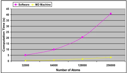
Figure 12. Timing performance plot of the LAMMPS software and the MD machine for the pairwise interaction computations on two nodes of the Maxwell.
0 5 10 15 20 25 30 35 40 45
32000 64000 128000 256000
Number of Atoms
C
o
m
p
u
ta
ti
o
n
T
im
e
(
s
)
Software MD Machine
to this clock frequency of the MD core, the clock fre-quency for the DDR2 SDRAM banks was 300 MHz. For benchmarking purposes, an all-atom Rhodopsin protein in solvated lipid bilayer was simulated with the Lennard-Jones forces, and the Coulombic forces via PPPM (parti-cle-particle particle mesh), incorporating SHAKE con-straints. This model contains counter-ions and a reduced amount of water to make a 32K atom system. The details of the simulation are as follows:
32,000 atoms for one time-step
LJ and Coulombic force cutoff of 10.0 Angstroms
Neighbor skin of 2.0 Angstroms
Average neighbors per atom = 372 atoms
NVT time integration
Table IV presents the timing performance figures of the LAMMPS software for the pairwise LJ and short-range Coulombic interaction computations of the above mentioned Rhodopsin protein system for one time-step on two nodes of the Maxwell machine (i.e. two software processes running on one host Intel Xeon CPU). The protein system was replicated in X, Y or Z dimensions to achieve the simulation of systems with up to 256,000 atoms, as presented in table IV.
TABLEIV.
TIMING FIGURES OF THE LAMMPSSOFTWARE FOR THE PAIRWISE I NTE-RACTION COMPUTATIONS ON TWO MAXWELL NODES
No. of Atoms
Computation Time (s) 32000 5.051342 64000 9.911402 128000 20.407846 256000 40.746851
For comparative purposes, table V shows the timing performance figures of the MD machine configured to operate in the same way as the pure software implementa-tion on two nodes of the Maxwell machine (i.e. two soft-ware processes running on one host Intel Xeon CPU and MD core instances on two Xilinx Virtex-4 XC4VFX100 FPGAs [44]). Note that the timing figures presented in table V do not include the I/O communication costs oc-curring during the data transfers between a host CPU and SDRAM banks.
TABLEV.
TIMING FIGURES OF THE MDMACHINE FOR THE PAIRWISE I NTERAC-TION COMPUTATIONS ON TWO MAXWELL NODES
No. of Atoms
Computation Time (s) 32000 0.379309 64000 0.785921 128000 1.674183 256000 3.130863
Fig. 12 plots the timing performance results of the pure software implementation and the MD machine for the pairwise interaction computations on two nodes of the Maxwell, as shown in tables IV and V, respectively. As it
can be seen, at all atom sytems, the MD machine operates faster than the pure software implementation. Note that both plots in fig. 12 show a quadratically increasing curve which is obviously much sharper for the pure software solution for the MD simulations.
Table VI provides the speed-up values of the MD ma-chine over the pure software implementation (LAMMPS) for the pairwise interaction computations of the systems with various numbers of atoms on two Maxwell nodes. Note that the MD machine outperforms the pure software implementation by 12x-13x.
TABLEVI.
LAMMPSVERSUS MDMACHINE SPEED-UP VALUES FOR THE I NTE-RACTION COMPUTATIONS ON TWO MAXWELL NODES
No. of Atoms
MD Machine Speed-Up 32000 13.32 64000 12.61 128000 12.19 256000 13.01
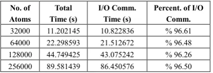
memory through, for instance, AMD’s Hypertransport, Intel’s Quick Path Interconnect or SGI’s NumaLink which offer bandwidths ranging from 15 to 25.6 GB/s, thus reducing communication overheads by at least 50x in comparison to our currently used communication link. This would result in performance gains of the MD ma-chine in overall over the pure software implementation by at least 8x-9x.
TABLEVII.
TIMING FIGURES OF THE MDMACHINE INCLUDING I/OC OMMUNICA-TION COSTS ON TWO MAXWELL NODES
No. of Atoms Total Time (s) I/O Comm. Time (s)
Percent. of I/O Comm. 32000 11.202145 10.822836 % 96.61 64000 22.298593 21.512672 % 96.48 128000 44.749425 43.075242 % 96.26 256000 89.581439 86.450576 % 96.50
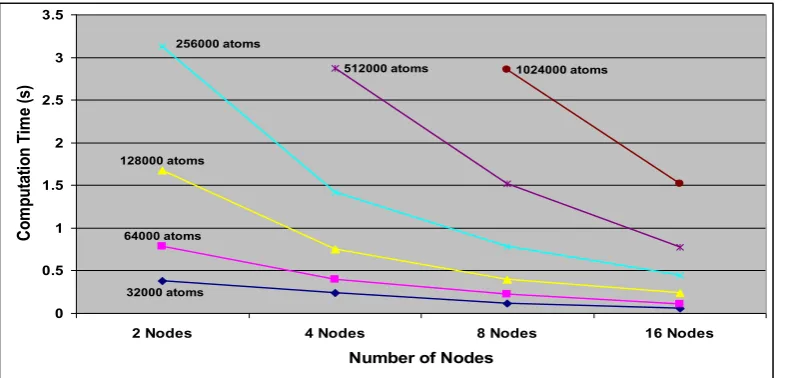
Tables VIII, IX and X show the comparative timing figures of the pure software implementation and the MD machine for the pairwise interaction computations of the Rhodopsin protein systems with up to over two million atoms for one time-step on 4, 8 and 16 nodes of the Maxwell machine, respectively. As it can be seen, the MD machine speed-up values for the pairwise interaction computations range from 10x to 14x. In addition, the effi-ciency and scalability of the MD machine on different numbers of nodes of the Maxwell is graphically repre-sented in fig. 13 with the timing values for the given numbers of atoms, as presented in tables V, VIII, IX and X. Note that the computational power of our MD ma-chine increases highly with the increasing number of the Maxwell nodes utilized.
TABLEVIII.
COMPARATIVE TIMING FIGURES OF THE LAMMPSSOFTWARE AND THE
MDMACHINE ON FOUR MAXWELL NODES
No. of Atoms SW Comp. Time (s) MD Machine Comp. Time (s)
MD Machine Speed-Up
32000 2.467384 0.237942 10.37
64000 4.959632 0.398379 12.45
128000 10.006767 0.748793 13.36
256000 20.08099 1.416626 14.18
512000 39.751763 2.869737 13.85
TABLEIX.
COMPARATIVE TIMING FIGURES OF THE LAMMPSSOFTWARE AND THE
MDMACHINE ON EIGHT MAXWELL NODES
No. of Atoms SW Comp. Time (s) MD Machine Comp. Time (s)
MD Machine Speed-Up
32000 1.202016 0.118279 10.16
64000 2.444738 0.220909 11.07
128000 4.856528 0.392149 12.38
256000 9.857229 0.781985 12.61
512000 19.563335 1.516907 12.90
1024000 40.567838 2.854312 14.21
TABLEX.
COMPARATIVE TIMING FIGURES OF THE LAMMPSSOFTWARE AND THE
MDMACHINE ON SIXTEEN MAXWELL NODES
No. of Atoms SW Comp. Time (s) MD Machine Comp. Time (s)
MD Machine Speed-Up
32000 0.610724 0.05701 10.71
64000 1.211133 0.111407 10.87
128000 2.406081 0.240549 10.00
256000 4.96922 0.441922 11.24
512000 9.783473 0.774302 12.64
1024000 19.683968 1.516273 12.98
2048000 40.287101 2.891285 13.93
Table XI shows the resource utilization of the MD core in a user FPGA. Note that the total number of the float-ing-point adder/subtractors in the MD core is 36 while the total number of the floating-point multipliers is 44. In addition, 8 floating-point comparators are utilised in our design. Furthermore, the floating-point adder/subtractors and comparators were entirely implemented in the slice logic. On the other hand, the floating-point multipliers were partially implemented in the DSP48 blocks on the FPGA. However, since each multiplier requires 4 DSP48 blocks and the total number of the DSP48 blocks in the user FPGA is just 160, it was only possible to map 40 of the multipliers to the DSP48 blocks while the rest of them were entirely implemented in the user logic.
TABLEXI.
RESOURCE UTILIZATION OF THE MDCORE IN A USER FPGA Used Available Utilization Number of
Occupied Slices 39,880 42,176 % 94 Total Number of 4
Input LUTs 69,622 84,352 % 82
Number of
Slice Flip Flops 43,021 84,352 % 51 Number of
FIFO16/RAMB16s 280 376 % 74
Number of
DSP48s 160 160 % 100
The accuracy in the computations was sufficient enough to carry out stable MD simulations but the accuracy could be improved if the single extended precision (i.e. width of 40-bit) was used for the floating-point numbers inside the design rather than the single precision (i.e. width of 32-bit) [45]. However, this precision increase would require higher amounts of slice logic and DSP48 blocks to implement the floating-point arithmetic units utilised in the MD core. Unfortunately, currently used Xilinx Virtex-4 XC4VFX100 FPGA chips cannot accommodate any higher resource demand as can be clearly seen in table XI.
Figure 13. Scaling performance of the MD machine on different numbers of nodes of the Maxwell for the given numbers of atoms 32000 atoms
64000 atoms 128000 atoms
256000 atoms
512000 atoms 1024000 atoms
0 0.5 1 1.5 2 2.5 3 3.5
2 Nodes 4 Nodes 8 Nodes 16 Nodes
Number of Nodes
C
om
pu
ta
tio
n
Ti
m
e
(s
)
used key would require doubling the size of the utilized Function Coefficients memories (see fig. 3). It is also impossible to realize the usage of 15-bit wide key considering the amount of Block RAMs available in the currently used Virtex-4 FX100 FPGA chip (refer to table XI).
IX. CONCLUDING REMARKS
The design and implementation of a FPGA core, namely MD core, carrying out all the necessary opera-tions to compute the non-bonded interacopera-tions in a MD simulation with the purpose of accelarating the LAMMPS MD software was presented in this paper. Our MD processor core comprised of 4 identical pipelines working independently in parallel to evaluate the non-bonded potentials, forces and virials was implemented on the nodes of a FPGA-based supercomputer, named Max-well, which consists of 64 Virtex-4 FPGA chips. This implementation allowed us to produce a special-purpose parallel machine for the hardware acceleration of the MD simulations. This machine yields higher computational power with the additional Maxwell nodes, making it highly scalable.
To our knowledge, our work is one of the few which present porting an existing production-grade MD soft-ware (i.e. LAMMPS) to FPGAs rather than an unopti-mized textbook MD code. As a novelty, our work is scaled up to many nodes on a FPGA-based supercompu-ter in contrast to other attempts to port a production-grade MD code on a reconfigurable computing platform. Fur-thermore, our design calculates the potential and virial values as opposed to the designs in these attempts.
The timing performance figures of the MD machine for the pairwise LJ and short-range Coulombic (via PPPM) interaction computations in the MD simulations of the solvated Rhodopsin protein systems with various numbers of atom show performance gains over the pure software implementation by factors of up to 13 on two nodes of the Maxwell machine. These MD machine speed-up values for the pairwise interaction computations were also maintained on different numbers of Maxwell
nodes. However, the overall timing performance of the MD machine is worse than the pure software implemen-tation due to the very high I/O communication costs of the data transfers between a host CPU and SDRAM banks. This case stems from the very poor data band-width between a host CPU and SDRAM banks which is a limitation caused by the hardware platform targeted in this implementation (i.e. Maxwell FPGA-based super-computer).
Nonetheless, if FPGA boards are integrated tighter into the host systems through, for instance, AMD’s Hyper-transport, Intel’s Quick Path Interconnect or SGI’s Nu-maLink, the bandwidth of the I/O communications would be greatly enhanced up to 25.6 GB/s, thus yielding much lower communication costs (i.e. at least 50x reduction in comparison with our currently used communication link). This would result in performance gains of the MD ma-chine in overall over the pure software implementation. On the other hand, the accuracy of the computations could be improved if the number of slices and DSP48 blocks available in the user FPGA (i.e. Xilinx Virtex-4 XC4VFX100) was higher. Furthermore, wider DSP48 blocks and larger block RAMs would also help to en-hance the computation accuracy. Solving the aforemen-tioned concerns with a better hardware implementation platform is the major plan for the future of this project.
REFERENCES
[1] M. P. Allen and D. J. Tildesley, “Computer Simulation of Liquids”, Oxford University Press, 1987.
[2] G. D. Fasman, “Prediction of Protein Structure and the Principles of Protein Conformations”, Plenum Press, New York, 1989.
[3] Z. R. Wasserman and C. N. Hodge, “Fitting an inhibitor into the active site of thermolysin: A molecular dynamics case study”, J. Proteins: Structure, Function, and Bioin-formatics, vol. 24, no. 2, pp. 227-237, Feb. 1996.
[5] D. I. Liao, E. Silverton, Y. J. Seok, B. R. Lee, A. Peter-kofsky and D. R. Davies, “The first step in sugar transport: crystal structure of the amino terminal domain of enzyme I of the E. coli PEP: sugar phosphotransferase system and a model of the phosphotransfer complex with HPr.”, J. Structure, vol. 4, no. 7, pp. 861-872, July 1996.
[6] N. L. Greenbaum, I. Radhakrishnan, D. J. Patel and D. Hirsh, “Solution structure of the donor site of a trans-splicing RNA”, J. Structure, vol. 4, no. 6, pp. 725-733, June 1996.
[7] D. C. Rapaport, “The Art of Molecular Dynamics Simula-tion”, Cambridge University Press, New York, 2004. [8] P. P. Ewald, “Evaluation of optical and electrostatic lattice
potentials”, Ann. Phys Leipzig, vol. 64, pp. 253-287, 1921. [9] L. Verlet, “Computer "Experiments" on Classical Fluids. I.
Thermodynamical Properties of Lennard-Jones Mole-cules”, Physical Review, vol. 159, no. 1, pp. 98-103, July 1967.
[10]D. Beeman, “Some Multistep Methods for Use in Molecu-lar Dynamics Calculations”, J. Computational Physics, vol. 20, pp. 130-139, Feb. 1976.
[11] M.E. Tuckerman, G.J. Martyna and B.J. Berne, “Reversi-ble multiple time-scale molecular dynamics”, J. Chemical Physics, vol. 97, no. 3, pp. 1990-2001, March 1992. [12]D. V. D. Spoel, E. Lindahl, B. Hess, G. Groenhof, A. E.
Mark and H. J. Berendsen, “GROMACS: Fast, flexible, and free”, J. Computational Chemistry, vol. 26, no. 16, pp. 1701-1718, Oct. 2005.
[13]GROMACS-4.0.7, “Download website for GROMACS
4.0.7”, available at http://www.gromacs.org, Dec. 2009. [14]J. C. Phillips, R. Braun, W. Wang, J. Gumbart, E.
Tajkhor-shid, E. Villa, C. Chipot, R. D. Skeel, L. Kale and K. Schulten, “Scalable molecular dynamics with NAMD”, J. Computational Chemistry, vol. 26., no. 16, pp. 1781-1802, Oct. 2005.
[15]NAMD-2.7b2, “Download website for NAMD 2.7b2”,
available at http://www.ks.uiuc.edu/Research/namd, Nov. 2009.
[16]LAMMPS, “Download website for LAMMPS”, available at http://lammps.sandia.gov, Jan. 2010.
[17]F. Toshiyuki, T. Makoto, M. Junichiro, E. Toshikazu and S. Duiichiro, “A Highly Parallelized Special-Purpose Com-puter for Many-Body Simulations with an Arbitrary Cen-tral Force: MD-GRAPE”, Astrophysical Journal, vol. 468, pp. 51-61, Sep. 1996.
[18]Y. Komeiji, M. Uebayasi, R. Takata, A. Shimizu, K. Itsuka-shi and M. Taiji, “Fast and Accurate Molecular Dynamics Sumulation of a Protein Using a Special-Purpose Comput-er”, J. Computational Chemistry, vol. 18, no. 12, pp. 1546-1563, Sep. 1997.
[19]S. Toyoda, H. Miyagawa, K. Kitamura, T. Amisaki, E. Hashimoto, H. Ikeda, A. Kusumi and N. Miyakawa, “De-velopment of MD Engine: High-Speed Accelerator with Parallel Processor Design for Molecular Dynamics Simula-tions”, J. Computational Chemistry, vol. 20, no.2, pp. 185-199, 1999.
[20]C. Wolinski, F. Trouw and M. B. Gokhale, “A preliminary study of molecular dynamics on reconfigurable comput-ers”, Proc. International Conf. Engineering Reconfigura-ble Systems and Algorithms, June 2003.
[21]R. Scrofano and V. K. Prasanna, “Computing Lennard-Jones potentials and forces with reconfigurable hardware”, Proc. International Conf. Engineering Reconfigurable Sys-tems and Algorithms, June 2004.
[22]R. Scrofano, M. B. Gokhale, F. Trouw and V. K. Prasanna, “Accelerating Molecular Dynamics Simulations with Re-configurable Computers”, IEEE Trans. on Parallel and
Distributed Systems, vol. 19, no. 6, pp. 764-778, June 2008.
[23]Y. Gu, T. VanCourt and M. C. Herbordt, “Improved inter-polation and system integration for FPGA-based molecular dynamics simulations”, Proc. International Conf. Field Programmable Logic and Applications, pp. 21-28, 2006. [24]Y. Gu, T. VanCourt and M. C. Herbordt, “Explicit design of
FPGA-based coprocessors for short-range force computa-tions in molecular dynamics simulacomputa-tions”, Elsevier Paral-lel Computing, vol. 34, no. 4, pp. 261-277, May 2008. [25]N. Azizi, I. Kuon, A. Egier, A. Darabiha and P. Chow,
“Re-configurable Molecular Dynamics Simulator”, Proc. IEEE Symp. Field-Programmable Custom Computing Machines, pp. 197-206, Apr. 2004.
[26]Y. Gu, T. VanCourt and M. C. Herbordt. “Accelerating molecular dynamics simulations with configurable cir-cuits”, Proc. International Conf. Field Programmable Log-ic and ApplLog-ications, pp. 475-480, Aug. 2005.
[27]LAMMPS, “LAMMPS manual”, available at
http://lammps.sandia.gov/doc/Manual.html, Jan. 2010. [28]L. Greengard and V. Rokhlin, “A Fast Algorithm for
Par-ticle Simulations”, J. Computational Physics, vol. 73, no.2, pp. 325-348, Dec. 1987.
[29]H. Q. Ding, N. Karasawa and W. A. Goddard, “Atomic level simulations on a million particles: The cell multipole method for Coulomb and London nonbond interactions”, J. Chemical Physics, vol. 97, no. 6, pp. 4309-4315, Sep. 1992.
[30]R. W. Hockney and J. W. Eastwood, “Computer Simulation Using Particles, Adam Hilger, 1988.
[31]T. Darden, D. York and L. Pedersen, “Particle mesh Ewald: An N⋅log(N) method for Ewald sums in large systems”, J. Chemical Physics, vol. 98, no. 12, pp. 10089-10092, June 1993.
[32]S. Plimpton, “Fast Parallel Algorithms for Short-Range Molecular Dynamics”, J. Computational Physics, vol. 117, no. 1, pp. 1-19, Mar. 1995.
[33]S. J. Plimpton, R. Pollock, M. Stevens, “Particle-Mesh Ewald and rRESPA for Parallel Molecular Dynamics Si-mulations”, Proc. SIAM Conf. Parallel Processing for Scientific Computing, Mar. 1997.
[34]E. L. Pollock and J. Glosli, “Comments on P3M, FMM, and the Ewald method for large periodic Coulombic sys-tems”, Computer Physics Communications, vol. 95, no. 2, pp. 93-110, June 1996.
[35]R. Baxter, S. Booth, M. Bull, G. Cawood, J. Perry, M. Par-sons, A. Simpson, A. Trew, A. McCormick, G. Smart, R.Smart, A. Cantle, R. Chamberlain and G. Genest, “Maxwell—a 64 FPGA supercputer”, Proc. NASA/ESA Conf. Adaptive Hardware Systems, pp. 287-294, 2007. [36]FHPCA, Edinburgh, U.K., “The FHPCA website”,
availa-ble at http://www.fhpca.org, 2010.
[37]Alpha Data Ltd., Edinburgh, U.K., “ADM-XRC-4FX Da-tasheet”, available at http://www.alphadata.co.uk./adm-adm-xrc-4fx.html, May 2007.
[38]Nallatech Ltd., Glasgow, U.K., “H100 Series Datasheet”, available at http://www.nallatech.com/meadiLibrary/ images/english/5595.pdf, May 2007.
[39]R. Baxter, S. Booth, M. Bull, G. Cawood, J. Perry, M. Par-sons, A. Simpson, A. Trew, A. McCormick, G. Smart, R. Smart, A. Cantle, R. Chamberlain and G. Genest, “The FPGA HPC alliance parallel toolkit”, Proc. NASA/ESA Conf. Adaptive Hardware Systems, pp.301-310, 2007. [40]FHPCA, Edinburgh, U.K., “PowerPoint presentation”,
available at http://www.fhpca.org/download/MRSC07-Mar07.ppt, Mar. 2007.
avail-able at http://www.unix.mcs.anl.gov/mpi/www/www3/ MPI_W time.html, 2009.
[42]OpenCores website, “Floating Point Adder and Multiplier”, available at http://opencores.org/project,fpuvhdl, 2009. [43]G. Marcus, P. Hinojosa, A. Avila and J. N. Flores, “A Fully
Synthesizable Single-Precision, Floating-Point Ad-der/Subtractor and Multiplier in VHDL for General and Educational Use”, Proc. IEEE International Caracas Conf. Devices, Circuits and Systems, pp. 319-323, Nov. 2004. [44]Xilinx Inc., San Jose, CA, “Virtex-4 datasheets”, available
at http://www.xilinx.com/products/silicon_solutions/fpgas/ virtex/virtex4/index.htm, May 2007.
[45]T. Amisaki, T. Fujiwara, A. Kusumi, H. Miyagawa and K. Kitamura, “Error evaluation in the design of a special-purpose processor that calculates nonbonded forces in mo-lecular dynamics simulations”, J. Computational Chemi-stry, vol. 16, no. 9, pp. 1120-1130, Sep. 1995.
[46]M. Chiu, M.C. Herbordt, “Efficient particle-pair filtering for acceleration of molecular dynamics simulation”, Proc. International Conf. Field Programmable Logic and Appli-cations, pp. 345-352, Aug. 2009.
[47]V. Kindratenko, D. Pointer, “A case study in porting a pro-duction scientific supercomputing application to a
reconfi-gurable computer”, Proc. IEEE Symp.
Field-Programmable Custom Computing Machines, pp. 13-22, April 2006.
Server Kasap received the B.Sc. degree in electrical and electronical engineering from the Middle East Technical Univer-sity, Turkey, in 2006 and the M.Sc. de-gree with distinction in system level integration from the University of Edin-burgh, U.K., in 2007, and the Ph.D. degree from the System Level Integra-tion Research Group of the School of Engineering at the University of Edinburgh, U.K., in 2010.
His research interests include high performance
reconfigurable architectures for bioinformatics and molecular
biology applications, high performance computing,
reconfigurable computing and hardware/software codesign. Dr. Kasap is a IEEE member. He is currently a senior lectur-er at the Electrical and Electronical Enginelectur-ering department of the European University of Lefke, Mersin-10, Turkey.
Khaled Benkrid received the "Inge-nieur d’Etat" degree in electronics engi-neering with distinction from Ecole Nationale Polytechnique d’Alger, Alge-ria, Alger, and the Ph.D. degree in com-puter science and an Executive MBA with distinction from Queen’s Universi-ty Belfast, Belfast, U.K.
With over ten years experience in FPGA hardware design, he has authored over 70 publications in major international journals and conference papers in the areas of high performance reconfigurable computing and electronic design automation with applications in digital signal processing, communication systems, bioinformatics and computational biology, financial computing, and scientific computing in gener-al.