Volume 2009, Article ID 821819,9pages doi:10.1155/2009/821819
Research Article
A Practical Scheme for Frequency Offset Estimation in
MIMO-OFDM Systems
Michele Morelli, Marco Moretti, and Giuseppe Imbarlina
Dipartimento di Ingegneria dell’Informazione, University of Pisa, Via Caruso 16, 56122 Pisa, Italy
Correspondence should be addressed to Marco Moretti,[email protected]
Received 27 June 2008; Revised 3 October 2008; Accepted 25 December 2008
Recommended by Mounir Ghogho
This paper deals with training-assisted carrier frequency offset (CFO) estimation in multiple-input multiple-output (MIMO) orthogonal frequency-division multiplexing (OFDM) systems. The exact maximum likelihood (ML) solution to this problem is computationally demanding as it involves a line search over the CFO uncertainty range. To reduce the system complexity, we divide the CFO into an integer part plus a fractional part and select the pilot subcarriers such that the training sequences have a repetitive structure in the time domain. In this way, the fractional CFO is efficiently computed through a correlation-based approach, while ML methods are employed to estimate the integer CFO. Simulations indicate that the proposed scheme is superior to the existing alternatives in terms of both estimation accuracy and processing load.
Copyright © 2009 Michele Morelli et al. This is an open access article distributed under the Creative Commons Attribution License, which permits unrestricted use, distribution, and reproduction in any medium, provided the original work is properly cited.
1. Introduction
Orthogonal frequency-division multiplexing (OFDM) is an attractive modulation technique for wideband wireless communications due to its robustness against multipath distortions and flexibility in allocating power and data rate over distinct subchannels. For these reasons, it is adopted in a variety of applications, including digital audio broadcasting (DAB), digital video broadcasting (DVB), and the IEEE 802.11a wireless local area network (WLAN) [1]. Combining OFDM with the multiple-input multiple-output (MIMO) technology is an effective solution to increase the capacity of practical commercial systems. The deployment of multiple antennas at both the transmitter and receiver ends can be exploited to improve reliability by means of space-time coding techniques and/or to increase the data rate through spatial multiplexing [2].
Similar to single-input single-output (SISO) OFDM, MIMO-OFDM is extremely sensitive to carrier frequency offsets (CFOs) induced by Doppler shifts and/or oscillator instabilities. The CFO destroys orthogonality among sub-carriers and must be accurately estimated and compensated for to avoid severe error rate degradations [3]. While CFO recovery is a well-studied problem for single antenna systems, only few solutions are available for MIMO-OFDM.
over disjoint time intervals. In this way, however, the preamble length grows linearly with the number of TX branches, thereby, increasing the system overhead. The use of chirp-like polyphase sequences is suggested in [11], while a training block composed of repeated PN sequences with good cross-correlation properties is employed in [12]. In both cases, the CFO estimate is obtained by cross-correlating the repetitive parts of the received preambles in a way similar to SISO-OFDM. This approach is also adopted in [13,14], where the pilot sequences are obtained by repeating Chu or Frank-Zadoff codes with a different cyclic shift applied at each TX antenna. Alternative criteria for MIMO-OFDM preamble design can be found in [15,16].
A subspace-based method for CFO estimation in MIMO-OFDM has recently been proposed in [17]. In this scheme, pilot symbols at different transmit antennas are frequency-division multiplexed (FDM) and placed over equally spaced subcarriers. The resulting preambles are characterized by an inherent periodic structure in the time domain which can be effectively exploited at the receiver to separate signals arriving from different TX antennas. This approach is reminiscent of the multiple-signal-classification (MUSIC)-based frequency recovery scheme employed in [18] in the context of orthogonal frequency division multiple access (OFDMA). The main advantage with respect to [18] is that in [17], the CFO estimate is obtained with reduced complexity by looking for the roots of a real-valued polynomial function. A root-based approach is also adopted in [19] after writing the CFO metric in polynomial form.
In this paper, the repetitive slots-based CFO estimator discussed in [8] is extended to MIMO-OFDM transmissions. In order to enlarge the frequency acquisition range, however, we decompose the CFO into a fractional part plus an integer part. The fractional CFO is computed first by cross-correlating the repetitive segments of the received preambles in a way similar to [8], while the integer CFO is subsequently estimated by resorting to maximum likelihood (ML) meth-ods. This results into an algorithm of affordable complexity which can estimate large CFOs and whose accuracy attains the relevant Cramer-Rao bound (CRB).
The rest of this paper is organized as follows.Section 2
describes the system model and introduces basic notation. In
Section 3, we review the joint ML estimation of the CFO and MIMO channel, whileSection 4 is devoted to the training sequences design and CFO recovery scheme. Simulation results are presented inSection 5and some conclusions are drawn inSection 6.
Notation 1. Matrices and vectors are denoted by boldface letters, withWN andIN being the DFT matrix and identity
matrix of order N, respectively. A = diag{a(n);n =
1, 2,. . .,N}denotes anN×Ndiagonal matrix with entries
a(n) along its main diagonal, while B−1 is the inverse of
a square matrix B. We use E{·}, (·)∗, (·)T, and (·)H for expectation, complex conjugation, transposition, and Hermitian transposition, respectively. The notation ·
represents the Euclidean norm of the enclosed vector, while
Re{x},|x|, and arg{x}stand for the real part, modulus, and principal argument of a complex numberx. Finally, [B]k,l
denotes the (k,l)th entry of a matrixB, whileλis a trial value of the unknown parameterλ.
2. System Model
We consider a MIMO-OFDM system withNT transmitting
andNRreceiving antennas. We denote byN the number of
available subcarriers which are enumerated fromn = 0 to
n=N−1 and callci=[ci(0),ci(1),. . .,ci(N−1)]Tthe
fre-quency domain pilot sequence at theith TX antenna. Before transmission, this sequence is converted in the time domain through an inverse discrete Fourier transform (IDFT) oper-ation and a cyclic prefix (CP) of length Ng is inserted
to avoid inter-block interference (IBI). The signal emitted from the ith TX branch arrives at the mth RX antenna after propagating through a multipath channel with discrete-time impulse responsehm,i = [hm,i(0),hm,i(1),. . .,hm,i(L−
1)]T, where L is a design parameter that depends on the duration of the transmit/receive filters and on the channel delay spread. Since one single oscillator is used for frequency conversion at both ends of the wireless link, the same CFO is assumed for all transmit/receive antenna pairs. We denote by xm = [xm(0),xm(1),. . .,xm(N −1)]T the time
domain samples available at themth RX antenna and define
Γ(ν)=diag{ej2πνk/N; 0≤k≤N−1}, whereνis the frequency
offset normalized by the subcarrier spacing. Assuming ideal timing recovery andNg ≥L, we have
xm=Γ(ν)sm+nm, (1)
where nm is an N-dimensional vector of AWGN samples
with zero-mean and varianceσ2
n, whilesm = [sm(0),sm(1),
. . .,sm(N−1)]T is the useful signal component, which is
modeled as
sm= NT
i=1
Aihm,i. (2)
In (2) , we have setAi=WHNCiFL, whereCi=diag{ci(n); 0≤
n≤N−1}collects the pilot sequence emitted by theith TX antenna, whileFLis anN×Lmatrix with entries
FL
n,l=e−j2πnl/N, 0≤n≤N−1, 0≤l≤L−1. (3)
InSection 3we show how to exploit vectors{xm; 1 ≤ m ≤
NR}for jointly estimating the CFOνand the MIMO channel
H = {hm,i; 1 ≤ m ≤ NR, 1 ≤ i ≤ NT}. In doing so, we
adopt the FDM training sequences suggested in [17], which optimize the performance of the LS channel estimator thanks to their shift orthogonality properties [9]. Such sequences are expressed by
ci(n)= ⎧ ⎪ ⎨ ⎪ ⎩
di(n) n=nQ+μi, 0≤n≤ N
Q−1
0, otherwise,
(4)
where Qis a power of two not smaller than NT,{μi} are
integer parameters satisfying 0 ≤ μ1 < μ2 < · · · < μNT <
Q, and di(n)} are pilot symbols with constant modulus |di(n)| =
Q/NT. In this way, the total energy allocated to
training amounts toET =Nand is equally split between the
3. Maximum Likelihood Frequency Estimation
Given the unknown parameters (H,ν), from (1), it turns out that vectors{xm}are statistically independent and Gaussian
distributed with meanΓ(ν)sm and covariance matrixσn2IN.
Hence, bearing in mind (2), the log-likelihood function (LLF) for (H,ν) takes the form
As a consequence of the FDM property of the employed training sequences, we observe thatAH
i1Ai2 =F
H
LCHi1Ci2FLis
the null matrix for anyi1=/i2. Using this fact, after neglecting
irrelevant terms independent ofH andν, we may rewrite the LLF as
joint ML estimate of the unknown parameters is the location whereΛ1(H,ν) achieves its global maximum. After standard
computations, the CFO estimate is found to be
andLLHis the following Cholesky decomposition:
LLH=
In the sequel, we refer to (7) as the maximum likelihood frequency estimator (MLFE). The following remarks are in order.
(1) Observing thatAHi Ai=FHLCHi CiFLwith rank{FL} =
L and rank {CHi Ci} = N/Q, it turns out that
rank{AH
i Ai} ≤min{L,N/Q}. SinceAHi Aihas
dimen-sionsL×L, a necessary condition for the existence of (AHi Ai)−1 in the right-hand-side of (9) is that L ≤
(2) By invoking the asymptotic efficiency property of the MLFE, the frequency estimate (7) is expected to be unbiased with an accuracy that approaches the corresponding CRB for large data records and sufficiently high signal-to-noise ratios (SNRs). Using the LLF in (5), it is found that [19]:
4.1. Problem Formulation. Direct maximization of g(ν) in (8) undertakes heavy computational burden. One possible way to reduce the system complexity is indicated in [19], where g(ν) is transformed into a real-valued polynomial function, and the CFO estimate is indirectly obtained by means of a polynomial rooting procedure. In this paper, we follow the alternative approach outlined in [8], by which a periodicity is first introduced in the MIMO training sequences, and CFO recovery is then accomplished by measuring the phase rotations between the repetitive parts of the received preambles. For this purpose, the sequences in (4) are modified so as to simultaneously satisfy the following constraints:
(C1) pilot symbols are equipowered, equispaced in the frequency domain and modulate distinct subcarriers at different TX antennas according to the FDM principle;
(C2) each vectorWH
Nci(i =1, 2,. . .,NT) of time domain
samples is obtained by the repetition ofRidentical segments, whereRis some power of two.
Condition C1 implies that the NT preambles remain
shift-orthogonal in the time domain, which is desirable to enhance the accuracy of the channel estimates, while condition C2 facilitates CFO recovery by ensuring that the preambles are periodic with periodP=N/R.
To proceed further, let Qbe a power of two withQ ≥
NT. Then, it can be easily shown that C1 and C2 are
subcarriers and their positions are shifted byRsubcarriers from one TX branch to the next. This amounts to putting
ci(n)=
M/NT to ensure that the total
energy allocated to training is still ET = N. It is worth
observing that the use of time-repetitive FDM training sequences for MIMO-OFDM has also been suggested in [16] to make the CRB of the frequency estimates independent of the channel realization. However, our design (14) is more general as it applies to any tripleN,NT,L), whereas in [16],
the number of subcarriers is constrained to be a multiple of
NTL. Recalling that in practical OFDM systemsNis always
a power of two, it turns out that the sequence design in [16] can only be adopted on condition that both NT andLare
powers of two.
As it is known, the use of OFDM preambles composed by
Rrepetitive slots restricts the acquisition range of the CFO estimator to±R/2 times the subcarrier spacing. To cope with such a drawback, we decomposeνinto afractional part, less thanR/2 in magnitude, plus aninteger partwhich is multiple ofR. The normalized CFO is thus rewritten as
ν=R(ε+η), (15)
where η is an integer parameter referred to as the integer CFO (ICFO), while ε is the fractional CFO (FCFO) and belongs to the interval (−1/2, 1/2]. Since the transmitted preambles remain periodic after passing through the channel (apart from the presence of thermal noise and from a phase shift induced by the CFO), each vector of received time domain samples can be decomposed intoRsegmentsxm =
[xT
m(0),xmT(1),. . .,xTm(R−1)]T, with
xm(r)=umej2πεr+nm(r), 0≤r≤R−1. (16)
In(16),umis aP-dimensional vector with elements
um(k)=ej2πνk/Nsm(k), 0≤k≤P−1, (17)
while{nm(r);r=0, 1,. . .,R−1}are statistically independent
Gaussian vectors with zero-mean and covariance matrix
σ2
nIP.
4.2. Estimation of the Fractional CFO. Our first goal is the estimation of ε based on the observations {xm}NmR=1.
Inspection of (16) reveals that this task is complicated by the presence of the nuisance vectors {um}. One possible
approach is to consider such vectors as deterministic but unknown parameters and proceed to the joint ML estimation of the parameter set (u,ε), withu = uT
1 uT2 · · · uTNR
T
. This approach has been used in [8] in the context of SISO-OFDM, and its extension to MIMO transmissions leads to the following FCFO metric:
where Rm(r) is the rP—lag sample correlation function
evaluated at themth RX branch, that is,
Rm(r)= N−1
k=rP
xm(k)xm∗(k−rP). (19)
The ML estimate of ε is eventually found by locating the global maximum of q(ε). Unfortunately, no closed form solution is available except whenR = 2. The more general case can be approached by an exhaustive search over the interval ε ∈ (−1/2, 1/2] which may be cumbersome in practice. For this reason, we suggest a suboptimal but simpler procedure which develops in two steps. In the first step a coarse FCFO estimate is obtained as
The rationale behind the above expression is easily under-stood after substituting (16) into (19). This yields
Rm(r)=(R−r)um2ej2πεr+Nm(r), (21)
where Nm(r) is a zero-mean disturbance term collecting
signal×noise and noise×noise interactions. Inspection of (21) reveals that, in the absence of noise, the right-hand-side of (20) is just the true FCFO. In order to improve the estimation accuracy, ε(c) is refined in the second step by
looking for an estimate of the residual errorΔε = ε−ε(c).
respect toΔεand assuming thatΔεis small enough such that sin[ϕ(mc)(r)−2πΔεr]ϕ(mc)(r)−2πΔεr, an estimate ofΔεcan
be computed in closed form as
Δε= 1
The final FCFO estimate is given by
ε=ε(c)+Δε. (24)
4.3. Estimation of the Integer CFO. If the normalized CFO is guaranteed to be less thanR/2 in magnitude, the quantityεR
can be regarded as an estimate ofν. Otherwise,νis expressed as in (15), and an estimate of the integer offset ηmust be found. This problem is now addressed using ML methods.
In order to compensate for the fractional offset ε, the received samples at each RX branch are first counter-rotated at an angular speed 2πεR/N . This produces the NR vectors
zm=[zm(0),zm(1),. . .,zm(N−1)]T, with
Substituting (1)-(2) into (25) and assuming ideal FCFO
statistically equivalent tonm. Vectors{zm}are next used to
get the joint ML estimate of (H,η). Bearing in mind (26), the corresponding LLF is found to be
Υ(H,η)= −NRN ln
Now, we observe thatAH
i Ai=FHLCiHCiFLis anL×Lmatrix
The concentrated likelihood function for η is found by substituting (29) into the right-hand-side of (27). Neglecting irrelevant terms independent ofη, we obtain
ψ(η)=
and the ML estimate ofηis computed as
which is determined by the stability of the transmitter and receiver oscillators. Recalling that Ai = WHNCiFL, after
standard manipulations, we may putψ(η) in the equivalent form
Once the ICFO is obtained as indicated in (31), an estimate of the CFO is computed from (15) in the form
ν=R(ε+η). (35)
In the sequel, we refer to (35) as the reduced complexity frequency estimator (RCFE).
4.4. Remarks. (1) As mentioned previously, matrixAHi Aiin
(28) is nonsingular provided thatL≤N/M. Such condition is more restrictive than the constraintL ≤ N/Q that was found in the previous section for MLFE. In particular, recalling that M = QR, it turns out that the maximum channel length that RCFE can manage isRtimes smaller than for MLFE.
(2) Assuming for simplicity that the ICFO has been perfectly estimated, from (35), it follows thatE{(ν−ν)2} =
R2·E{(ε−ε)2}. Since parameters (u,ε) are jointly estimated
through ML methods, we expect that E{(ε−ε)2} asymp-totically approaches the corresponding CRB. The latter is provided in [8] and reads
sdenotes the average signal power at each RX branch,
that is,
The frequency MSE is thus given by
E(ν−ν)2= 3
(3) The computational load of RCFE can be assessed as follows. Computing the correlations{Rm(r)}rR=−11 in (19)
requires a total of 2(R−1)(2N−1) real operations (additions plus multiplications) for each RX branch, while 8NR(R−
1) operations are needed to obtain Δεin (23). Quantities
Zm(n) in (33) are computed through anN-point DFT for
each receiving antenna, with a corresponding complexity of 5NRN log2N. Finally, evaluating ψ(η) in (34) needs
additional 8NLNTNR/Moperations for eachη. The overall
complexity of RCFE is summarized in the first row ofTable 1, where a distinction has been made between the FCFO and ICFO recovery tasks, and we have denoted byNη=2|η|max+
1 the number of hypothesized ICFO values.
Table1: Complexity of FCFO and ICFO estimation schemes.
FCFO recovery ICFO recovery
RCFE 2NR(R−1)(2N+ 3) NRN(5 log2N+ 8LNTNη/M)
PBFE 4NRNQ+ 30(Q−1)3 NRN(5 log2N+ 4NT)
CBFE 4NR(3N−2P−1)
proposed in [12]. Actually, both schemes employ training preambles composed byRrepetitive parts and operate in two steps. A coarse estimateε(c)is firstly computed by CBFE in a
way similar to (20), and it is next refined by evaluating the quantity
Δε= 1
πRarg
NR
m=1 R(c)
m
R
2
. (39)
The final CFO estimate is obtained asνCBFE =R(ε(c)+Δε),
and its MSE is given by [12]
EνCBFE−ν2
= 2
π2 σ2
n/σs2
NRN.
(40)
Comparing this results with (38), we see that the loss (in dB) with respect to RCFE is 10·Log[4(1−1/R2)/3], which
approaches 1.25 dB for large values ofR. Furthermore, since no ICFO estimation is attempted in [12], the estimation range of CBFE is restricted to |ν| ≤ R/2, while RCFE can cope with CFOs as large as ±N/2. The overall complexity of CBFE is shown in the third line ofTable 1. Compared to FCFO recovery by means of RCFE, the computational saving of CBFE is in the order ofR/3.
5. Simulation Results
Computer simulations have been run to check and extend the analytical results of the previous sections. The simulation scenario is summarized as follows.
5.1. Simulation Model. The investigated MIMO-OFDM system has N = 1024 subcarriers and operates in the 5 GHz frequency band. The signal bandwidth is 5 MHz, corresponding to a subcarrier distance of approximately 4.9 kHz. The sampling period is Ts = 0.2 microsecond,
so that the useful part of each OFDM block has length 0.205 millisecond. Each channel is characterized by L =
12 independent Rayleigh fading taps with an exponentially decaying power delay profile
Ehm,i()2
=σh2·exp
−4
L
, =0, 1,. . .,L−1.
(41)
In (41), the constant σh2 is chosen such that the channel
power is normalized to unity, that is,E{hm,i2} =1. A new
channel snapshot is generated at each simulation run and kept fixed over the training period. Vectorshm,iare assumed
to be statistically independent for different TX/RX antenna
10−6 10−5 10−4
MSE
0 3 6 9 12 15 18
SNR (dB) RCFE
PBFE CBFE
EMCB
NT=3,NR=2
Figure1: MSE of the FCFO estimators versus SNR withNT=3 and
NR=2.
pairs . The training sequences employed by RCFE are given in (14), where we have set R = 8 and Q = 4. In this way, each TX antenna transmits a total of 32 pilot symbols which are randomly taken from a QPSK constellation with power|di(n)|2 =32/NT. ParametersNT andNR are varied
throughout simulations to assess their impact on the system performance.
Comparisons are made between RCFE, CBFE, and the polynomial-based frequency estimator (PBFE) proposed in [17]. This scheme employs the training sequences defined in (4) and performs initial ICFO recovery by maximizing the following cost function:
ψPBFE(η)=
NR
m=1
NT
i=1
N/Q−1
n=0
Xm
nQ+μi+η2 (42)
over the set η ∈ {−Q/2,−Q/2 + 1,. . .,Q/2 −1}, with
{Xm(n); 0 ≤ n ≤ N − 1} being the N-point DFT
of xm. After ICFO compensation, the fractional CFO is
eventually estimated by looking for the roots of a real-valued polynomial function that is obtained by applying the MUSIC principle. As mentioned in [17], the estimation range of PBFE is|ν| ≤Q/2. Its computational requirement is mainly ascribed to the need for evaluating the correlation matrix of the received time domain samples and is summarized in the second row ofTable 1.
5.2. Performance Assessment. Figure 1compares the
perfor-mance of the fractional CFO estimators in terms of their MSE E{(ν−ν)2} versus the signal-to-noise ratio at each receiving antenna. The latter is defined as SNR = σ2
s/σn2,
whereσ2
nis the noise power, andσs2is given in (37). Marks
10−6 10−5 10−4
MSE
0 3 6 9 12 15 18
SNR (dB) NT=2
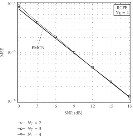
NT=3 NT=4 EMCB
RCFE NR=2
Figure2: Accuracy of RCFE versus SNR withNT=2, 3, 4 andNR=2.
ease the reading of the graphs. The number of TX and RX antennas is NT = 3 and NR = 2, respectively. The same
training sequences are used for both CBFE and RCFE, while PBFE employs the pilot design specified in (4) withQ=32 and {μ1,μ2,μ3} = {0, 1, 5}. This means that the number
of pilot symbols transmitted by each TX antenna is 32 for all the considered schemes. As suggested in [17], the pilot symbols{di(n)}for PBFE belong to a Chu sequence. The
CFO is randomly generated at each simulation run with uniform distribution within the interval [−0, 4; 0.4), which corresponds to havingη=0 andε=ν/R. For the time being, we concentrate on the accuracy of the FCFO estimates and assume ideal ICFO recovery for both RCFE and PBFE. We use the average CRB to benchmark the performance of the considered schemes. The latter corresponds to the extended Miller and Chang bound (EMCB) [20] and is obtained by numerically averaging the right-hand-side of (12) with respect to the channel statistics. Inspection ofFigure 1reveals that RCFE outperforms the other schemes, and its accuracy is close to the EMCB at all investigated SNR values. As predicted by the theoretical analysis shown in (38) and (40), the loss of CBFE with respect to RCFE is approximately 1.25 dB. Looking at the system complexity, fromTable 1, it turns out that in the considered scenario, RCFE requires a total of 57 500 operations for FCFO recovery, while PBFE and CBFE need 1 156 000 and 24 000 operations, respectively. Combining these figures with the results ofFigure 1indicates that RCFE is superior to PBFE in terms of both estimation accuracy and processing load, while CBFE is a valid solution when limiting the computational requirement is an issue of concern.
Figure 2illustrates the impact of the number of transmit antennas NT on the accuracy of RCFE. The simulation
10−6 10−5 10−4
MSE
0 3 6 9 12 15 18
SNR (dB) NR=2
NR=3 NR=4 EMCB
RCFE NT=3
Figure3: Accuracy of RCFE versus SNR withNT=3 andNR=2, 3, 4.
scenario is the same as in Figure 1, except that nowNT =
2, 3 or 4. As it is seen, the frequency MSE is virtually independent ofNTand the same occurs for the EMCB. Such
behavior can be ascribed to the fact that signals emitted by different TX antennas combine incoherently at each RX branch, so that higher values of NT do not result into a
corresponding increase of the array gain. As it is known, array gain exploitation by means of multiple TX antennas requires channel knowledge at the transmitter in conjunction with suitable precoding techniques.
Figure 3shows how the performance of RCFE is affected by the numberNRof receiving antennas. In such a case,NTis
fixed to three whileNR=2, 3 or 4. As predicted by (38), the
estimation accuracy improves withNR,and this trend is also
evident in the EMCB. The physical reason behind such SNR advantage is that the presence of multiple receiving antennas increases the length of the data recordx=[xT
1,x2T,. . .,xTNR]
T
used for CFO recovery. This provides the system with an array gain of 10·Log(NR) dB.
The performance of the ICFO estimators is illustrated in
Figure 4in terms of probability of failure Pf = Pr{η /=η}
versus SNR. Comparisons are made between RCFE and PBFE using the same simulation setup of Figure 1. The RCFE metric defined in (34) is evaluated forη∈ {−2,−1, 0, 1, 2}, while PBFE looks for the maximum ofψPBFE(η) over the set
η∈ {−16,−15,. . ., 15}. In this way, the estimation range is
10−4 10−3 10−2 10−1 100
Pf
−18 −15 −12 −9 −6
SNR (dB) RCFE
PBFE
NT=3,NR=2
Figure4: Probability of failure versus SNR for RCFE and PBFE with
NT=3 andNR=2.
a judicious design of parameterQ. Specifically, decreasingQ
alleviates the computational requirement at the expense of a reduced CFO acquisition range.
6. Conclusions
We have addressed the problem of training-assisted CFO recovery in MIMO-OFDM systems. To reduce the compu-tational burden required by the exact ML solution, we have divided the CFO into a fractional part plus an integer part and have designed FDM pilot sequences that are periodic in the time domain. The fractional CFO is estimated in closed form by measuring the phase rotations between the repetitive parts of the received preambles, while the integer CFO is estimated in a joint fashion with the MIMO channel matrix by resorting to the ML principle. The proposed scheme has affordable complexity and exhibits improved performance with respect to existing alternatives. For these reasons, we believe that it provides an effective approach for frequency synchronization in beyond third generation (3G) wideband MIMO-OFDM transmissions.
References
[1] “Wireless LAN medium access control (MAC) and physical layer (PHY) specifications, higher speed physical layer exten-sion in the 5 GHz band,” 1999.
[2] G. L. St¨uber, J. R. Barry, S. W. Mclaughlin, Y. E. Li, M. A. Ingram, and T. G. Pratt, “Broadband MIMO-OFDM wireless communications,”Proceedings of the IEEE, vol. 92, no. 2, pp. 271–294, 2004.
[3] T. Pollet, M. van Bladel, and M. Moeneclaey, “BER sensitivity of OFDM systems to carrier frequency offset and Wiener phase noise,”IEEE Transactions on Communications, vol. 43, no. 234, pp. 191–193, 1995.
[4] Y. Yao and G. B. Giannakis, “Blind carrier frequency offset estimation in SISO, MIMO, and multiuser OFDM systems,” IEEE Transactions on Communications, vol. 53, no. 1, pp. 173– 183, 2005.
[5] X. Ma, M.-K. Oh, G. B. Giannakis, and D.-J. Park, “Hopping pilots for estimation of frequency-offset and multiantenna channels in MIMO-OFDM,”IEEE Transactions on Communi-cations, vol. 53, no. 1, pp. 162–172, 2005.
[6] T. M. Schmidl and D. C. Cox, “Robust frequency and timing synchronization for OFDM,” IEEE Transactions on Communications, vol. 45, no. 12, pp. 1613–1621, 1997. [7] M. Morelli and U. Mengali, “An improved frequency offset
estimator for OFDM applications,” IEEE Communications Letters, vol. 3, no. 3, pp. 75–77, 1999.
[8] M. Ghogho, A. Swami, and P. Ciblat, “Training design for CFO estimation in OFDM over correlated multipath fading channels,” in Proceedings of the 50th Annual IEEE Global Telecommunications Conference (GLOBECOM ’07), pp. 2821– 2825, Washington, DC, USA, November 2007.
[9] I. Barhumi, G. Leus, and M. Moonen, “Optimal training sequences for channel estimation in MIMO OFDM systems in mobile wireless channels,” inProceedings of the International Zurich Seminar on Broadband Communications: Accessing, Transmission, Networking, pp. 441–446, Zurich, Switzerland, February 2002.
[10] A. van Zelst and T. C. Schenk, “Implementation of a MIMO OFDM-based wireless LAN system,” IEEE Transactions on Signal Processing, vol. 52, no. 2, pp. 483–494, 2004.
[11] A. N. Mody and G. L. St¨uber, “Synchronization for MIMO OFDM systems,” inProceedings of IEEE Global Telecommuni-catins Conference (GLOBECOM ’01), vol. 1, pp. 509–513, San Antonio, Tex, USA, November 2001.
[12] C. Yan, S. Li, Y. Tang, and X. Luo, “Frequency synchronization in MIMO OFDM system,” in Proceedings of the 60th IEEE Vehicular Technology Conference (VTC ’04), vol. 3, pp. 1732– 1734, Los Angeles, Calif, USA, September 2004.
[13] T. C. W. Schenk and A. van Zelst, “Frequency synchronization for MIMO OFDM wireless LAN systems,” inProceedings of the 58th IEEE Vehicular Technology Conference (VTC ’03), vol. 2, pp. 781–785, Orlando, Fla, USA, October 2003.
[14] J. Zheng, J. Han, J. Lv, and W. Wu, “A novel timing and frequency synchronization scheme for MIMO OFDM system,” in Proceedings of the International Conference on Wireless Communications, Networking and Mobile Computing (WiCOM ’07), pp. 420–423, Shanghai, China, September 2007. [15] H. Minn, N. Al-Dhahir, and Y. Li, “Optimal training signals
for MIMO OFDM channel estimation in the presence of frequency offset and phase noise,” IEEE Transactions on Communications, vol. 54, no. 10, pp. 1754–1759, 2006. [16] M. Ghogho and A. Swami, “Training design for multipath
channel and frequency-offset estimation in MIMO systems,” IEEE Transactions on Signal Processing, vol. 54, no. 10, pp. 3957–3965, 2006.
[17] Y. Jiang, H. Minn, X. Gao, X. You, and Y. Li, “Frequency offset estimation and training sequence design for MIMO OFDM,” IEEE Transactions on Wireless Communications, vol. 7, no. 4, pp. 1244–1254, 2008.
[19] Y. Jiang, X. You, X. Gao, and H. Minn, “MIMO OFDM frequency offset estimator with low computational com-plexity,” in Proceedings of IEEE International Conference on Communications (ICC ’07), pp. 5449–5454, Glasgow, Scotland, June 2007.