ABSTRACT
ROBINSON, BRENT ROSS. Models for Prediction of Surface Vibrations from Pile Driving Records. (Under the direction of Dr. Mohammed A. Gabr.)
This study compares high strain dynamic testing measurements taken near the top of a driven pile to peak particle velocities on the ground surface and sound levels detected in the air some distance from the pile during driving. Based on a sample of installation records from 16 piles driven at the Marquette Interchange Project in Milwaukee, Wisconsin, a series of peak particle velocity plots versus distance, energy and scaled distance were created using traditional horizontal distance and rated hammer energy. These plots were modified using the seismic distance, the diesel hammer potential energy from the calculated stroke, and the energy transferred to the pile top. Incorporating these measurements tended to reduce some of the scatter in the data. More importantly, it was also discovered that components of peak particle velocity in the ground can be well correlated to the total pile resistance measured by dynamic testing. A plot of total resistance versus depth often independently yields the same shape curve as a plot of at least one component of peak particle velocity versus depth. A simple mathematical attenuation model is proposed as an initial step toward utilizing this relationship to predict at least one component of ground motions. Measured peak
Biography
Brent Robinson was born in Battle Creek, Michigan in August, 1976. He received his BS in Civil Engineering, in May 1999, from Case Western Reserve University in Cleveland, Ohio. After graduation he joined GRL Engineers, Inc. as a research and field engineer. While with GRL, he performed high strain dynamic tests and other quality control tests on deep foundations and on construction sites around the U.S. and around the world. His work also included teaching nondestructive pile testing methods to engineers from other firms, in individual and classroom settings.
Acknowledgments
This study would not have been possible without permission to use the Marquette Interchange data from the Wisconsin Department of Transportation and the Federal Highway Administration. In addition to the project’s future benefits to the city of Milwaukee, they have also created a valuable data set for the future.
I would like to acknowledge my colleagues at GRL Engineers, Inc., particularly Patrick Hannigan, who organized the PDA testing, and who, along with Mark Rawlings, acquired and analyzed much of the PDA data included in this study. I would also like to thank Dr. Frank Rausche for taking a chance on a young engineer and guiding me through a five year adventure at his firm. The work of the Wagner Komurka Group and Milwaukee Transportation Partners is also gratefully acknowledged, as they collected driving and vibration records and helped facilitate the data transmission. Finally, the analyses in this thesis could not have been performed without the skill and dedication of the contractors and laborers who installed and assisted in the testing of each pile.
TABLE OF CONTENTS
LIST OF TABLES... vi
LIST OF FIGURES ... vii
CHAPTER 1: INTRODUCTION ... 1
1.1 PILE DRIVING: ANALYTICAL TECHNIQUES ... 2
1.2 PROBLEM STATEMENT... 4
1.3 OBJECTIVES ... 4
1.4 ORGANIZATION ... 4
CHAPTER 2: LITERATURE REVIEW AND BACKGROUND ... 6
2.1 GROUND VIBRATIONS ... 6
2.1.1 Conceptual Propagation Model... 6
2.1.2 Vibration Thresholds ... 8
2.1.3 Other Analysis Methods ... 14
2.2 CODES AND FREQUENCY BASED LIMITS ... 16
2.3 CASE HISTORIES... 19
2.4 HIGH STRAIN DYNAMIC PILE TESTING... 24
2.5 PILE DRIVING NOISE ... 29
2.6 SUMMARY... 33
CHAPTER 3: THE MARQUETTE INTERCHANGE ... 34
3.1 GENERAL PROJECT INFORMATION... 34
3.1.1 Soil ... 35
3.1.2 Piles... 35
3.1.3 Hammers ... 36
3.1.4 Pile Driving Records... 37
3.1.5 Vibration Monitoring... 37
3.1.6 High Strain Dynamic Testing Device ... 38
3.1.7 Data Reduction... 39
3.2 DATA FOR THIS STUDY ... 40
3.2.1 Subsurface Characteristics ... 41
3.2.2 Vibration Data... 44
3.2.3 Driving Records and PDA Data... 46
3.2.4 Coordinating vibration and PDA data... 50
3.3 SUMMARY... 52
CHAPTER 4: PREDICTION OF PEAK PARTICLE VELOCITY... 54
4.1 TRADITIONAL VIBRATION ANALYSIS FOR PILE DRIVING... 54
4.1.1 Vibrations versus Frequency... 54
4.1.2 Vibrations versus Distance ... 55
4.1.3 Vibrations versus Hammer Energy... 58
4.1.4 Scaled Distance Plots... 61
4.2 ANALYSIS WITH PDA VELOCITY DATA ... 66
4.3. ANALYSIS USING PDA TOTAL RESISTANCE. ... 72
4.3.1 Estimating PPV from RTL... 76
CHAPTER 5: PREDICTION OF SOUND LEVELS... 85
5.1 TRADITIONAL NOISE ANALYSIS FOR PILE DRIVING... 85
5.1.1 Noise versus distance... 85
5.1.2 Scaled Distance... 87
5.2 COMPARING PDA DATA TO NOISE LEVELS ... 91
5.3 MATHEMATICAL MODEL... 95
5.4 SUMMARY... 99
CHAPTER 6: SUMMARY AND CONCLUSIONS... 100
CHAPTER 7: FUTURE RESEARCH... 105
7.1 PEAK PARTICLE VELOCITIES IN THE SOIL ... 105
7.2 NOISE... 107
7.3 WAVE EQUATION PROGRAMS FOR PILE DRIVING... 107
CHAPTER 8: REFERENCES ... 108
APPENDIX... 112
DRIVING RECORDS ... 113
LIST OF TABLES
Table 1. Classification of Earth Materials by Attenuation Coefficient (Woods and Jedele,
1985) ... 11
Table 2. City of Milwaukee (2006) Nuisance Code Limits on Transient Vibrations... 17
Table 3. Measured transfer and hammer efficiencies for various hammer types. ... 28
Table 4. Summary of piles for this report... 41
Table 5. Vibration Monitoring Test Details... 45
Table 6. Longitudinal PPV correlated to toe velocity and peak velocity in pile. ... 71
Table 7. R2 values when PPV/VRTL is plotted versus normalized distance ... 79
Table 8. Simple model parameters... 80
Table 9. R2 values for correlation of total resistance to peak overpressure, all piles. ... 94
LIST OF FIGURES
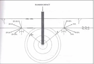
Figure 1. Conceptual Sketch of Waves Generated by Pile Driving (from Woods, 1997)... 7
Figure 2. Transmission, Reflection and Refraction of a Compressive (P) and Shear Wave (SV) in a Layered Media (from Woods, 1997)... 8
Figure 3. Sample Log PPV vs. log distance plot (Woods and Jedele, 1985)... 13
Figure 4. PPV vs. Energy Plot for many vibration sources (modified from Woods and Jedele, 1985). ... 13
Figure 5. Scaled Distance Plot from Woods and Jedele (1985). N = 1.525 ... 14
Figure 6. Typical threshold for people and buildings ... 18
Figure 7. Scaled Distance Plots from Previous Studies... 20
Figure 8. Seismic (or slope) distance plot for Peak Particle Velocities (from Hope and Hiller, 2000) ... 22
Figure 9. Rated Hammer Energy versus Peak Particle Velocities (Hope and Hiller, 2000). 22 Figure 10. Scaled Distance Plot (Hope and Hiller, 2000)... 23
Figure 11. HSDPT transducers on a pile to be tested during restrike... 24
Figure 12. Typical early driving force-velocity (F-V) curve from a driven pipe pile. ... 27
Figure 13. Pile Driving Noise versus distance plots from prior studies. ... 31
Figure 14. Delmag D46-32 at Static Load Test Site E ... 36
Figure 15. Junttan HHK 10A driving a pile on a non static load test site ... 37
Figure 16. Vibra-tech Everlert VE monitoring device and ballast at Static Load Test Site F38 Figure 17. Summary of SPT N-Values for Four Static Load Test Sites... 43
Figure 18. Results from Vibration Monitoring Program: Maximum PPV vs. time ... 47
Figure 19. Results from vibration monitoring: Maximum Sound Level vs. time... 47
Figure 20. PDA screenshot of later blow from SLT-B-12-1. Force (F), Velocity (V), Energy (E) and Displacement (D) ... 48
Figure 21. Selected PDA Data versus Depth of Pile Penetration ... 50
Figure 22. Selected PDA Result and Vibration Data plotted versus time. ... 51
Figure 23. PDA and Vibration Data after filtering to match data points... 52
Figure 24. Vibration data compared to threshold levels. ... 56
Figure 25. Vibration data plotted versus horizontal distance from source. ... 57
Figure 26. Vibration data plotted versus seismic distance (note: models modified from Figure 25)... 57
Figure 27. Vibration data plotted versus rated energy of the hammers. ... 59
Figure 28. Vibration data plotted versus potential energy calculated from stroke. Diesel hammer sites only. ... 60
Figure 29. Vibration data plotted versus energy transferred to the PDA gages (EMX)... 61
Figure 30. Scaled Distance Plots using Horizontal Distance and Rated Energy ... 63
Figure 31. Scaled Distance Plots using Seismic Distance and Potential Energy from Stroke ... 64
Figure 32. Scaled Distance Plots using Seismic Distance and Transferred Energy from Stroke ... 65
Figure 34. Vibration and calculated toe velocity versus time... 68
Figure 35. Peak Velocity due to Impact compared to PPV components. ... 69
Figure 36. Toe velocity compared to PPV components. ... 70
Figure 37. PPV and PDA velocities versus time. SLT-E-16-2... 72
Figure 38. PPV and Total Resistance from PDA. SLT-E-16-2 ... 73
Figure 39. Vertical PPV and Total Resistance from PDA. SLT-E-16-2 ... 74
Figure 40. Vertical PPV and "Mirrored" Total Resistance from PDA. SLT-E-16-2... 75
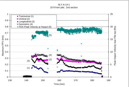
Figure 41. PPV and Total Resistance for SLT-A-14-1. Note the longitudinal velocity... 75
Figure 42. Correlation of Normalized distance to normalized velocity... 77
Figure 43. Model results versus measured PPV data in PPV-seismic distance space... 78
Figure 44. Range of possible model results using statistics from Table 8... 81
Figure 45. Slope of model, k, versus Horizontal Distance for all piles with R2 greater than 0.6... 82
Figure 46. Model slope, k, versus Pile Impedance, Z, for all piles with R2 greater than 0.6. 82 Figure 47. Horizontal distance plot, piles driven with Junttan HHK-10A hydraulic hammer. ... 86
Figure 48. Horizontal distance plot, piles driven with Delmag D46-32 diesel hammer. ... 87
Figure 49. Junttan HHK 10-A Noise levels compared to diagonal distance from hammer to microphone. ... 88
Figure 50. Delmag D46-32 Noise levels compared to diagonal distance from hammer to microphone. ... 89
Figure 51. Delmag D46-32 Noise levels compared to potential energy scaled distance ... 89
Figure 52. Junttan HHK-10A noise levels compared to transferred energy scaled distance. 90 Figure 53. Delmag D46-32 noise levels compared to transferred energy scaled distance. ... 90
Figure 54. Correlation of peak overpressure to pile velocity at impact peak. ... 93
Figure 55. Correlation of peak overpressure to total resistance... 93
Figure 56. Correlation of total resistance to peak overpressure... 94
Figure 57. Correlation of peak overpressure to total resistance., SLT B-12-2. ... 95
CHAPTER 1: INTRODUCTION
For millennia, impact driven piles have been used to support structures constructed on weak or unstable soils. Most piles over the centuries were made of timber, and driven to depth using human or animal power. The Roman empire was connected by roads paved by stones and bridges supported by piles. As the industrial revolution dawned, inventors and
construction contractors turned their steam and diesel engines to the process of driving piles. No longer limited by the weights a group of people, horses or oxen could lift (or by the number of people the constructor could afford to hire), ram weights could be made larger and from cast iron or steel. The time between hammer blows could also be reduced, and the energy imparted to the pile could, at least in theory, be more carefully controlled.
Similarly, as concrete technology advanced and steel manufacturing developed, the piles themselves could be made to nearly any length, from materials that allowed higher loads to be placed over their cross sectional areas. As load bearing capacity increased, the size of the hammer required to install them generally increased, as well. As larger hammers were introduced, engineers attempted to make the most of them, designing piles with yet higher loads.
And so the cycle of pile design and installation technology continues to this day. Pile driving has, however, became something of a victim of its own success. By allowing more marginal sites to be developed, cities and other areas became more densely populated. As these populations grew, the number of people and existing structures located around new construction or reconstructed sites increased as well. In the middle 20th century, the installation techniques of pile driving began to come under scrutiny.
these structures will be understandably alarmed and annoyed by the shaking of their building and the repeated noise from the nearby construction activities. In some cases, these
vibrations will also cause the occupants to look closely at the structure itself, and take careful notice of any cracks or other damage to the existing structure.
Thus, the act of pile driving and the vibrations it causes is generally a two pronged problem: the annoyance created by the noise and vibration, and the possibility of damage to nearby structures due to the vibrations. For driven piles to continue to be a viable design alternative, the latter should be unquestionably avoided and the former should be minimized to reduce public outcry and resistance to a particular project. The challenge, then, is to minimize vibrations or to keep them within an acceptable level.
A topic to the impact of pile driving involves vibration in water due to pile installation. In the last decade or two, there has been increased concern regarding the effects of pile driving on fish behavior and habitat. Changes in fish behavior and even fish kills have been
observed at sites, particularly in shallow waters where fish hatchlings are found. While related and a topic for concern, this aspect of the impact of vibrations from pile driving will not be addressed in this thesis.
Thus, there is some value in being able to predict prior to construction what vibrations in the air (sound), soil, or water will result from pile driving activity. If it can be shown that the probability of damage due to vibrations are minimized or that the noise due to a particular pile-hammer system is below regulated thresholds, then pile driving may be accepted in a place where another, possibly more expensive foundation system is being strongly
considered.
1.1 PILE DRIVING: ANALYTICAL TECHNIQUES
tests, where a series of weights are placed on the pile top and the displacement is measured. Prediction methods were then developed, using soil mechanics theory and tests on soil samples to estimate the axial load carrying capacity of a single pile. Once these predictions and static load tests were complete, quality control on site for additional piles was and is often provided by counting and recording the number of blows required to move the pile a certain distance. In the last thirty years, high strain dynamic pile testing (HSDPT) has been used to combine both a record of driving and a capacity estimate on an actual pile at the time of driving. These measurements are obtained by installing strain transducers and
accelerometers near the pile top and monitoring the transmission of compressive stress waves generated by the hammer impact.
As axial static capacity prediction developed, the question of whether a particular pile could be economically and successfully driven to a desired ultimate capacity with a particular driving system arose. Wave equation technology developed over the last fifty years as a pre-construction tool. An algorithm was developed to predict the stress in pile, energy
transferred to pile, and set per blow for a given resistance and hammer type. Studies have been performed (Rausche et al., 2004) to check the ability of wave equation analyses to predict the quantities measured by HSDPT, showing that if the system is modeled correctly, these quantities can be predicted well.
1.2 PROBLEM STATEMENT
This research focuses on methods currently used to predict peak particle velocities (a measure of the magnitude of vibration) in soils and sound levels transmitted through the air near pile driving operations. First, a literature review will be conducted to determine the current state-of-practice in both pile driving vibration and sound prediction methods and to review the information obtainable from widely used techniques to monitor pile installations (high strain dynamic testing, HSDPT). Previous field and numerical studies will be
reviewed, as well as the combination of the monitoring techniques with vibration records.
The results of this review will then be applied to a site in the downtown area of Milwaukee, Wisconsin, USA where pile driving was performed. Here, on a small subset of more than eighty full scale driven test piles, soil borings, traditional pile driving records, high strain dynamic test data, noise data and vibration data will be combined. This data set is somewhat unique, in that high strain dynamic test data are available for nearly every hammer blow, and vibration and noise maxima are available in 15 second increments (or every five to twelve blows) for the initial installations of many piles.
1.3 OBJECTIVES
The existing methods of noise and vibration prediction will then be compared to results from this field installation. At the same time, HSDPT data will be used to check the ability of other measured and calculated quantities to predict ground vibrations and noise levels. From these comparisons, mathematical models will be proposed. Finally, the study will conclude with a summary of the major results, final conclusions, and recommendations for future research or studies.
1.4 ORGANIZATION
Chapter 2 reviews existing ground vibration and noise prediction models as applied to pile
driving. It also briefly reviews the quantities that can be calculated or measured from HSDPTs, which measure compressive stress wave propagation through the pile.
Chapter 3 summarizes the Milwaukee test pile program, focusing on the six static load test
sites. It will summarize the pile types driven, the hammers used, the soil types encountered and the HSDPT and vibration data available.
Chapter 4 compares the ground vibration data to existing models, and the pile driving
records to vibration data. A model will be proposed and other observations will be made.
Chapter 5 compares the noise data to existing models and analysis methods, and the pile
driving records to collected noise data. An improved model will be proposed and other observations will be made.
Chapter 6 summarizes the major findings andconcludes this portion of the study.
CHAPTER 2: LITERATURE REVIEW AND BACKGROUND
The literature for noise and sound propagation due to pile driving extends back almost forty years. Much of the work has focused on the prediction of maximum velocities or sound levels accumulated over the entire driving event. Historically, this comes from vibration studies done for explosives in the mining and highway industries, where the events tend to be single, and not continuous or repetitious over long periods. The mining standards were extended to impact and vibratory driven piles by Wiss (1981).
While a number of papers have been published studying the vibrations in soil due installation of piles with vibratory hammers (see Borden and Shao, 1995; Morris, 1998, Viking, 2002), those will not be focused on here. Instead, only vibrations due to installation of piles using impact hammers will be discussed.
2.1 GROUND VIBRATIONS
Researchers and practitioners have approached the problem of vibrations due to pile driving in a few different ways. These range from conceptual models to empirical plots of vibration versus energy or distance to create an envelope of maximum expected values, to other theories and techniques. This section will briefly review this literature.
2.1.1 Conceptual Propagation Model
refracted into the adjoining layer as presented by Woods (1997). See Figure 1and Figure 2 for a conceptual sketch of this model.
Rayleigh and Love waves are generated once the shear and compression waves generated by the pile driving reach the surface. These waves propagate along the air-soil boundary, and tend to have higher amplitudes than the compressive and shear body waves. These surface waves tend to cause the most damage in earthquakes or other dynamic events, because of their higher amplitudes and thus larger distortion of structures. (Woods, 1997). Given full time histories of vibrations at a given site and knowing a distance from the source far enough to allow the waves to separate, these different waves can be identified in a particular record.
Figure 2. Transmission, Reflection and Refraction of a Compressive (P) and Shear Wave (SV) in a Layered Media (from Woods, 1997).
The model in Figure 1, however, is currently better suited to the conceptual understanding of the problem than careful numerical studies of actual pile driving records. In heavily layered soils, the reflection and refraction of multiple shear and compression waves becomes difficult to manage. Similarly, while one could calculate the expected arrival time of waves based on a soil’s compressive and shear wave speeds, the amplitude of the resulting vibration would be largely unknown without a separate model for attenuation of those waves in the soil. Thus, the methods currently in common use are still highly empirical.
2.1.2 Vibration Thresholds
collected, which can range in the tens or hundreds for a day of blasting and hundreds or thousands for a day of pile testing. Much of the guidance on pile driving vibration monitoring and thresholds are adopted directly from the blasting industry.
In his seminal study on pile driving vibrations, Wiss (1981) discusses a few of the common models of vibration attenuation, many of which are still used and shown in literature today. By examining the literature of structural damage due to blasting (for example, Edwards and Northwood, 1960 and Wiss, 1974), Wiss noted that peak particle velocity tended to correlate with structural damage and disturbance of the public. Wiss (1981) also noted that as the energy of the blast increased, the peak particle velocity increased and as the distance from source to monitoring area increased, peak particle velocity decreased. These relationships are empirically modeled in Equations 1 and 2.
a
CE
PPV = Equation 1
In Equation 1, PPV = Peak particle Velocity (in/s), C and a are the intercept (in/s) and slope (log units) of a best fit line, and E is the impact energy (ft-lbs). For piles, this E is typically assumed to be the hammer’s rated energy, or a value usually defined by the hammer manufacturer as the weight of the impact ram multiplied by the maximum achievable drop height
n
kD
PPV = − Equation 2
and practitioners still tend to use either the horizontal distance or seismic distance, or in a few cases, show both results.
Wiss (1981) then observed the effects of distance and energy can be combined into a single equation, such as Equation 3. This is a so-called scaled distance relationship, that was again originally developed for blasting and introduced in Wiss (1967). The parameters K and N are similar to (but not the same as!) those in Equation 2. Wiss (1981) the value of N should be between 1 and 2, averaging around 1.5.
N
E D K
PPV = ( / ) Equation 3
Equations 2 and 3 are meant to partially capture the effects of attenuation or damping of the wave front in an elastic media as the distance increases. A different attenuation model that considers geometric spreading of the wave in a half space with material damping was developed by Bornitz in 1931 and is shown in Equation 4.
) (D Do
n
o o e
D D A
A − −
−
⎟⎟ ⎠ ⎞ ⎜⎜ ⎝ ⎛
= α Equation 4
In Equation 4, A is the amplitude of PPV at a distance D of interest, Ao and Do are known
amplitude at a base distance, respectively, n is a function of the type of wave transmitted and
α is the attenuation coefficient. The exponent n can be shown to be 1 for body waves (shear and compression) in the ground spreading spherically. On the surface, body waves have an n of 2, while the n for Rayleigh waves is ½.
frequencies of 5 and 50 Hz; other frequencies can be calculated using a simple ratio as shown in Equation 5.
1 2 1 ` 2
f f
α
α = Equation 5
where α1 is the known attenuation at a frequency f1 (5 or 50 Hz) and α2 is the unknown
attenuation at frequency f2.
Table 1. Classification of Earth Materials by Attenuation Coefficient (Woods and Jedele, 1985)
Attenuation Coefficient, α (1/ft) Soil Class
5 Hz 50 Hz
Description of Material
I 0.003 – 0.01 0.03 – 0.10 Weak or soft soils (shovel penetrates easily);
loessy soils, dry or partially saturated peat and muck, mud, loose beach or dune sand, recently plowed ground, soft spongy forest or jungle
floor, organic soils, topsoil
II 0.001 – 0.003 0.01 – 0.03 Competent Soils (can dig with shovel): most
sands, sandy clays, silty clays, gravel, silts, weathered rock
III 0.0001 – 0.001 0.001 – 0.01 Hard soils (cannot dig with shovel, must use
pick to break up): dense compacted sand, dry consolidated clay, consolidated glacial till,
some exposed rock
IV <0.0001 <0.001 Hard, competent rock (difficult to break with
hammer); bedrock, freshly exposed hard rock
energy, pile penetration and soils encountered will all affect the measured vibrations. In most cases, these vibrations will be harmless, so the methods laid out in Equations 1 through 4 are meant to predict upper bound, or maximum vibration magnitudes. These maxima are then compared to code requirements or other commonly used charts that correlate vibration levels to structural damage. Thus, the models outlined above are not meant to predict all vibration levels, just the most critical ones.
Results of these studies are generally plotted on log-log scale plots, with PPV the dependent variable and distance, energy or scaled distance the independent variable. Figure 3 through Figure 5 show the most common plots used in the vibration literature. It is these that will be used as a starting point for the analyses in this study. A sample plot of peak particle velocities (maxima only) versus distance is recreated in Figure 3 from the work of Woods and Jedele (1985). This data set was collected on a site where sheet piles are driven with a Linkbelt 440 diesel hammer, which had a reported rated energy of 13,200 ft-lbs. For the
pseudo-attenuation model in Equation 3, n was 1.476; for the pseudo-attenuation damping model in Equation 4, α was 0.0319 and n was 0.5.
Figure 4 shows maximum peak particle velocities versus energy as shown in Woods and Jedele (1985). Again, these are from a number of different types of vibration sources, not just pile driving. For reference, the range of hammer energies from the most recent hammer database for the GRLWEAP wave equation program is included along the bottom.
0.001 0.01 0.1 1 10
1 10 100 1000
Distance from Source (ft)
Peak
P
a
rt
ic
le
V
e
lo
ci
ty
(
in/s)
Woods and Jedele, 1985, Linkbelt 440 Closed End Diesel
Psuedo-Attenuation
Attenuation Damping
Figure 3. Sample Log PPV vs. log distance plot (Woods and Jedele, 1985).
0.0001 0.001 0.01 0.1 1 10 100
100 1000 10000 100000 1000000 10000000
Energy (ft-lbs)
PPV
(
in/s)
Distance 10 ft; n=1.4-1.53 Distance 100 ft, n=1.4-1.53 Distance 10 ft
Distance 100 ft
RANGE OF HAMMER RATED ENERGIES (PDI, 2006)
0.0001 0.001 0.01 0.1 1 10 100
0.001 0.01 0.1 1 10 100
Scaled Distance (Distance/SQRT(Energy) in ft/(ft-lb)0.5)
PP
V (
in
/s
)
All data points, n=1.41-1.53; 10, 100, 1000 ft
Distance 10 ft
Figure 5. Scaled Distance Plot from Woods and Jedele (1985). N = 1.525
2.1.3 Other Analysis Methods
Outside of the log-log plots of velocities versus distance or energy, a few other researchers have proposed other ways to predict peak particle velocities in the ground due to impact pile driving. These include finite element studies, methods that use displacements generated by other programs, or the response spectra currently used in structural engineering for
earthquakes.
To predict the vibration records, Ramshaw et al. (1998) used a triangular impact force pulse of 5 seconds in duration. This input was placed into a finite element model that was assumed to have two layers with purely elastic properties. The model generated compressive, shear and Rayleigh waves, and produced an expected ground movement in the radial direction of motion. The authors reported the match between measured and predicted values was satisfactory, although the peak magnitude of the vibration at 54 feet from the pile was over predicted by a factor of 6 and the signal at 18 ft appeared to be overly damped. As more full time histories become available, this type of analysis may become more common.
Svinkin (1999) suggested a method of vibration prediction that uses “impulse-response functions” to predict vibrations versus time. Impulse-response functions are generated by an onsite, preconstruction test program where a mass is dropped on the surface and the response of the soil is measured. Once these functions are determined through reverse analyses, Svinkin (1999) suggests using the displacement versus time histories at various points along the pile from a wave equation program such as GRLWEAP (Pile Dynamics, Inc., 2006) to predict the dynamic force input into the soil. This dynamic force versus time function is then used in conjunction with the site specific impulse-response functions to estimate the
horizontal and vertical vibration versus time histories at the site.
Massarsch (2005) has laid out the beginnings of a prediction model that considers the one dimensional compression wave travel and individual transfer of energy along the side of the pile and at the toe. Noting the limitations of the distance/energy attenuation methods
described earlier, Massarsch (2005) develops equations to calculate conservative estimates of the stress at the pile toe and the maximum velocity in the pile. These are then used to predict maximum velocities at the pile toe and along the shaft that are transmitted into the
surrounding soils.
To estimate the velocity transmitted into the soils, the stress at the base in the pile are
wave velocity. The shear velocities’ strain dependence helps to model the plastic zone that occurs at the pile soil interface, and can reduce the shear wave velocity by up to 70% (Massarsch, 2005). To determine maximum vibrations on the surface in the far field, equation 4 is used.
The method of Massarsch (2005) shows promise, but needs to be refined, calibrated and verified prior to more widespread adoption. In U.S. practice, it is also unusual (but, with the growing requirement of shear wave velocity measurement for seismic site classification, becoming more common) to measure shear wave velocities on sites.
Finally, Dowding (1996) advocates a movement toward response spectra analysis as is used in earthquake engineering and structural dynamic analyses. In this case, for a particular input time history, the relative displacement response of a single degree of freedom system can be generated. The time history would be an acceleration or velocity versus time history for a
particular pile driving vibration site. Given the response spectra, the engineer can proceed with structural design of the building or checks to see whether cracking or damage to an existing building. This method, however, requires measurement and recording of the most significant time histories, or at least an ability to accurately scale up a particular time history. This requires the ability of the monitoring equipment to automatically select and record the most critical time histories.
2.2 CODES AND FREQUENCY BASED LIMITS
The methods above arose from complaints or concerns about damage due to vibrations, and, as a means of limiting disputes and liability of contractors, owners and engineers. Not surprisingly, most cities and states now have codes that deal specifically with vibration and noise.
limitations on vibrations and noise levels are codified. These limitations are placed at the local, state and federal levels. For example, AASHTO (1990) recommends limiting peak particle velocities to between 0.5 and 1 inch/second to minimize the risk of damage for buildings in good repair. The State of Wisconsin (2006), based on a widely used recommendation by Siskind et al. (1980) to the Office of Surface Mining, uses a set of thresholds based on both the peak particle velocity and frequency. Similarly, as a part of its nuisance ordinances, the City of Milwaukee (2006), defines the acceptable limits of transient vibration (such as those due to pile driving), based on displacement amplitude levels. The limits are recreated in Table 2Figure 6.
Table 2. City of Milwaukee (2006) Nuisance Code Limits on Transient Vibrations.
Frequency (Hz) Peak Displacement Amplitude(in)
2 0.1 5 0.01 10 0.005 20 0.0018 30 0.001 40 0.0008 50 0.0006 60 0.0005
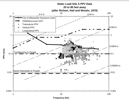
Research has also been performed that determines at what peak particle velocities people start to notice, and at what velocities they start to become worried. These thresholds were presented by Reiher and Meister (1931) and were recreated in Richart et al. (1970). They determined that peak particle velocities of just below 0.01 in/s were barely noticeable, while velocities of 0.1 in/s or more often caused alarm.
frequency, taking advantage of the integral relationship between the three quantities. The dashed lines at an angle in Figure 6 are a displacement scale plotted logarithmically. The City of Milwaukee’s data are plotted on the displacement scale, although peak particle velocities plotted on the same chart will also be subject to the same thresholds.
Vibration Limits for People and Structures Including PPV and Displacement Amplitude
(after Richart et al., 1970)
0.001 0.01 0.1 1 10
1 10
Frequency (Hz)
PPV
(
in/
s
)
0.001 0.01 0.1 1 10
1 10
100 100
City of Milwaukee Code OSM/Wisconsin DOT
Barely Noticeable to People Troublesome to People
0.4 in 0.04 in
0.004 in
0.0004 in
0.00004 in
Figure 6. Typical threshold for people and buildings
limited to only 0.2 in/s up to 10 Hz and linearly increasing (on the log-log plot) to 1 in/s at 100 Hz (Dowding, 1996).
These codes are just a sampling, but include the codes in effect for the project used for this study, which will be described in Chapter 3. From this short review, the vibration standards generally serve two purposes: to limit the effects on the occupants of neighboring structures (nuisance ordinances) and to limit the likelihood of damage to the structures themselves.
2.3 CASE HISTORIES
Over the years, a number of reports have included the results of vibration studies due to impact vibrations. Many vibration studies occur in private practice every day, but these are not available for or included in this review. Instead, those available in literature are briefly surveyed.
Linehan et al (1992) investigated the response of a natural gas pipeline to construction activities. This included sheet pile driving with a vibratory hammer, H-Pile driving with an impact hammer, as well as demolition of a wall. The pile was an HP14x73 that was 58 ft long at final penetration and driven with a diesel hammer with a rated energy of between 23,000 and 30,000 ft-lbs. Vibrations were monitored on the soil surface and on the pipeline, where it was noted that those in the vertical or east-west direction tended to be maximum. It was concluded that the settlements observed during driving of the sheet piles and H-Piles were more detrimental to the structure than the vibrations themselves. Figure 7 shows this data along with that presented by Woods and Jedele (1985).
two different places: on the concrete foundations of existing structures and on free soil. In all cases, the free soil vibrations were higher than those measured on the concrete.
0.0001 0.001 0.01 0.1 1 10 100
0.001 0.01 0.1 1 10 100
Scaled Distance (Distance/SQRT(Energy) in ft/(ft-lb)0.5)
PPV
(
in/s
)
Woods and Jedele (1985) Partial Data Linehan et al. (1992) Data
Prost and Meyer (1984) Data Singh and Knoebel (1993) on Soil Singh and Knoebel (1993) on Concrete Heckman and Hagerty (1978) Upper Bound Jedele (2005) Upper Bound
Woods and Jedele (1986) Best Fit, N=1.525 Svinkin (1999) Upper Bound
Svinkin (1999) Lower Bound
Figure 7. Scaled Distance Plots from Previous Studies.
In 2005, Jedele used the scaled distance relationship in equations 3 and 4 to extend the results of Woods and Jedele, 1985. To predict upper bound values, it was observed that the values of K= 0.137 and n = 1.27 fit the data best when D is in feet and E is in ft-lbs. This upper bound curve (but not the new data points) is included in Figure 7, along with an upper bound suggested by Heckman and Hagerty (1978), where K = 0.23 and n=1. Finally, Svinkin (1999) suggested a range of curves shown as upper and lower bound lines in Figure 7 based on the approximate velocity of the pile head at impact. The selection of scaled distance for this velocity is arbitrary set to be very small (0.001 ft/(ft-lb)0.5).
20 feet, as well as encasing the top 8 feet in a larger diameter steel shell filled with sand. The piles were driven with a Vulcan 01 hammer, which has a rated energy of 15,000 ft-lbs. Based on AASHTO (1990) guidelines, the peak particle velocities were limited to 0.5 to 1.0 in/s for buildings in good repair. Most of the data points fell under the Woods and Jedele (1985) curve shown in Figure 7, with peak particle velocities ranging from around 0.1 to 0.4 in/s at scaled distances ranging from 0.11 to 0.57 ft/(ft-lbs)0.5.
Figure 8. Seismic (or slope) distance plot for Peak Particle Velocities (from Hope and Hiller, 2000)
Figure 10. Scaled Distance Plot (Hope and Hiller, 2000).
2.4 HIGH STRAIN DYNAMIC PILE TESTING
High strain dynamic pile testing (HSDPT) is performed during initial installation or during a restrike of a driven pile. Two to four strain transducers and two to four accelerometers are attached near the top of the pile to measure strain and acceleration records over a set period of time, usually on the order of 50 to 300 milliseconds. An example of an instrumented pile is shown in Figure 11 (the ruler is to collect pile set measurements for restrike purposes). The instrumentation is connected to a field computer on the ground that serves as the data acquisition and data processing system (Pile Dynamics, Inc., 2003).
The HSDPT testing equipment collects and records strain and acceleration records for every (or selected, if the operator so chooses) hammer blow. The equipment internally processes the data and then calculates quantities such as stresses in the pile, energy transferred to the gage location, estimates of axial pile capacity at the time of testing, and forces, velocities and displacements of the gage location. A few of the quantities used in this study will be
described here.
In most cases, the quality of HSDPT data is monitored by the operator from the calculated force and velocity versus time curves. Figure 12 shows a sample force-velocity plot. From the strain and acceleration records measured by the gages, force and velocity are calculated from Equations 6 and 7.
) ( )
(t EA t
F = ε (6)
Where:
F(t) is the calculated force at the gage location as a function of time E is the elastic modulus of the pile material at the gage location A is the area of the pile at the gage location
ε(t) is the measured axial strain in the pile at the gage location
∫
= a t dt
t
v( ) ( ) (7)
Where:
v(t) is the calculated velocity at the location of the accelerometer a(t) is the measured acceleration at the location of the accelerometer dt is the time between recorded data points
the force and velocity will can be plotted proportionally using the pile’s impedance, as shown in Equation 8.
) ( ) (t Zv t
F = (8)
Where:
Z is the pile impedance as shown in equation 9
cA c
EA
Z = =ρ (9)
c is the compressive wave speed of the pile material
ρ is the mass density of the pile material
For piles, which are by no means infinite, the force and velocity will only remain
proportional until the traveling stress wave meets resisting forces. Practically, this usually means that proportionality will hold for HSDPT until the peak of the pulse created by impact. If there is any significant side friction, the velocity and force curves will begin to deviate and proportionality at the gage location will no longer hold. The record in Figure 12, for
example, was taken during early, easy driving where the pile had not penetrated significantly into soils that generate significant shear resistance. As such, proportionality between the force and velocity is maintained until the wave reflects off the toe at a time of 2L/c, where L is the length from the gages to the pile toe. This point in the record is the amount of time required for the wave to travel from the gages down the pile, to reflect off the pile toe, and to return to the gage location. As is noted in Rausche et al. (1985) and Pile Dynamics, Inc. (2003), the time of maximum impact (T1) and the time 2L/c later (T2) where the toe
reflection is seen are very useful in determining resistance, stresses elsewhere in the pile, and other quantities.
VT2, VMX). By integrating the velocity vs. time curve, a maximum and final calculated displacement (DMX and DFN) can be determined. By integrating the product of force and velocity over time, as shown in Equation 10, a curve of energy versus time can be generated. Taking the maximum point on that energy curve gives EMX.
T2: 2L/c T1: impact
maxima
Figure 12. Typical early driving force-velocity (F-V) curve from a driven pipe pile.
∫
= tend
dt t v t F Max EMX
0 ( ) ( ) (10)
A hammer’s transfer or global efficiency is usually defined as the maximum energy transferred to the pile location (EMX) divided by the hammer’s rated energy (which was discussed in Section 2.1.2). The transfer efficiency takes into account losses due to guide friction, losses in the cushion, losses due to friction and myriad other sources of energy loss. Alternatively, if other devices such a radar gun or proximity switches (but not a PDA) are used to measure the ram velocity prior to impact, a hammer efficiency can also be calculated. This hammer efficiency is built into hammer models in most wave equation programs.
Rausche (2000) summarized typical transfer efficiencies of various types of hammers based on the results of a large number of dynamic pile tests. Similarly, the GRLWEAP program (Pile Dynamics, Inc., 2006) includes hammer efficiencies based on ram velocity
Table 3. Measured transfer and hammer efficiencies for various hammer types.
Transfer efficiency: Steel Piles
Transfer efficiency: Concrete Piles
Hammer Efficiency Hammer
Type
Average (%) Range (%) Average (%) Range (%) (%)
Single Acting Air/Steam
55 40-70 40 30-55 67
Single Acting Diesel
31 25-50 24 15-35 80
Hydraulic Manufacturer and System Dependent
For open end diesel hammers, where the behavior of the ram is dictated by gravity, the stroke of the ram (the ram’s drop height) can be estimated using the Saximeter equation (as
discussed in Rausche 2000) shown in equation 11.
L
h T g
STK = 2 −
8 (11)
Where:
g is the acceleration due to gravity
T is the time between hammer impacts in seconds
hL is an empirically correlated estimate of losses due to friction, gas compression, etc.
Finally, Rausche et al. (1985) derived the Case method estimate of static resistance by breaking up the total resistance experienced by a pile into static and dynamic components. The static component is what is of most interest to the typical practitioner. The total resistance, RTL, is derived in Rausche et al. (1985) using the pile impedance, the measured forces FT1 and FT2, and the measured velocities VT1 and VT2. The dynamic component of resistance, Rd, is modeled as being linearly proportional to the toe velocity, Vtoe, using a Case
factor, J as shown in Equation 12.
) 1
1 * ( *
*Z V J Z VT FT RTL
J
Rd = c toe = c + − (12)
The PDA does not explicitly calculate toe velocity as a quantity for output. However, knowing equation 12 and outputting VT1, FT1 and RTL, this value can be manually calculated for any particular blow.
The PDA can calculate a number of other stresses, displacements, accelerations, and resistances for a given pile record. For this study, only those above are focused on. To review, there are three forces (FT1, FT2, FMX), four velocities (VT1, VT2, VMX, Vtoe), the
transferred energy (EMX), the hammer stroke (STK), and the maximum displacement (DMX). Other quantities could be investigated in future studies.
2.5 PILE DRIVING NOISE
With pile driving comes the sound of the hammer impacting the pile. The study of sound transmission is an enormous field, and the mitigation and hazards of loud continuous and transient sounds has been studied for decades. From worker protections in settings with loud industrial equipment to protection of homeowners through traffic noise barriers to controlling the noise from surrounding cubicles to the tuning of a new concert hall, the field of
does not look survey the entirety of the field of sound control and acoustics. Hopefully, a brief review will suffice.
One simple way to predict the attenuation of sound is to perform an analysis similar to those used for vibrations: plot versus distance. Similar to the vibration studies, this results in a log-log plot with considerable scatter, but will allow the engineer to plot upper bound thresholds and continue with design.
As shown in Figure 13, previous studies of noise from pile driving presented in Dowding (1996) show a relatively wide range of possible sound levels that tend to attenuate with distance. The data shown in Figure 13, from Linehan and Hannen (1984) are from a site in Phoenix where piles were driven through cemented sands and gravels to near refusal
conditions. Dowding (1996) calls the Phoenix data outliers, attributing the high noise levels to the very hard driving and the low frequency air pressure transducers employed to measure sound.
Outdoor sound propagation modeling methods are summarized by Kurze and Anderson (2006). Propagation of sounds in an outdoor environment are affected by the height of the source (in this case, the pile driving hammer) and the receiver (the vibration monitoring equipment), as well as reflection and refraction of the waves off buildings, the ground, and in the air as wind or temperature changes. The sound attenuates naturally as the pressure disturbance expands outward (much like ground vibrations), but can also be attenuated by natural or manmade barriers or absorbed by the atmosphere. Clearly, there are plenty of variables to complicate the analysis!
The relation between the sound produced by the source, LW, and the sound detected, Lp, at a
distance, d, and angle from the source, Φ is shown in Equation 13 (Kurze and Anderson, 2006).
) , ( )
( )
,
(d φ L D φ D A d φ
The correction factors in equation 13 are for the direction of the source, DI, which for pile
driving should be zero since the sound is in not focused in a particular direction (like a speaker or air horn, for example) if the hammer is in a free field. DΩ can be estimated using equation 14. It accounts for situations where the source and receiver are at different heights, and the source itself is very close to the ground. Instead of radiating spherically, the sound waves from the source can only radiate over half a sphere. The correction factor A is a function that takes into account any other elements, such as walls or hills, in the path of the sound wave that can attenuate or amplify its intensity.
1.0E-06 1.0E-05 1.0E-04 1.0E-03 1.0E-02 1.0E-01
1 10 100 1000
Distance (ft) P e a k ove rpressu re ( p si ) 50 60 70 80 90 100 110 120 130 140 150 S o u n d P res su re L e ve l ( d B )
95% Linehan and Hannen (1984)
Avg Linehan and Hannen (1984)
Alsup (1981)
Linehan and Hannen (1984) Data Range
Figure 13. Pile Driving Noise versus distance plots from prior studies.
⎥ ⎦ ⎤ ⎢ ⎣ ⎡ + + − + + =
Ω 2 2
2 2 ) ( ) ( 1 log 10 R s R s h h d h h d
In equation 14, d is the horizontal distance from source, S, to receiver, R, hS is the height
of the source and hR is the height of the receiver. This factor will only be needed when the
hammer is very close to the ground.
The transfer function, A, in equation 14 takes into account attenuation in free space over ground, as well as reflections from buildings, walls, and other barriers. For attenuation, the model can assume either straight line ray paths or account for refraction of the sound wave due to changes in atmosphere. This latter correction requires some knowledge of the
temperature and wind gradient with altitude. Equation 15 shows the attenuation function, A, of spherically radiating sound waves, where dS-R is the straight line (diagonal) distance from
the source to the receiver and d0 is a distance of 3.28 ft (1 m).
2 0
2
4 log 10
d d
A= π S−R (in dB) (15)
Other attenuation factor formulations exist, but, since good data on ground surface, buildings and other built structures is not easily obtainable for this study, they will be assumed to be negligible. For a more detailed discussion, see Kurze and Anderson (2006).
To fully use Equation 13, the source intensity, Lw, must be estimated. To do so, the change
in pressure due to the hammer impact on the pipe pile must also be estimated. The simplest analysis is to assume an infinitely long tube (Vér, 2006). As the hammer impacts the tube, a compression occurs at a particular velocity, vo(t), much like a piston at the end of the pipe.
This compresses the air filling, for the current discussion, a rigid walled tube. The air has a density, ρ, and a wave speed, c. As shown in Equation 16, the pressure as a function of time can be determined.
c t v t
For a typical dynamic pipe pile test, the peak velocity during impact is around 10 ft/s. The mass density of air is 0.0022 slugs/ft3 (0.07 lb/ft3 specific weight) and the compressive wave speed in air is approximately 1128 ft/s. Given these parameters, the maximum sound
pressure is 0.18 psi, or 156 dB (relative to a base overpressure of 2.9 x 10⁻⁹ psi for calculating decibel level).
Of course, this is a gross oversimplification, since the pile is not infinitely long, there is resistance along the side of the pile, reflections of sound can occur inside the pile itself, and other sound generators, such as the hammer, must be considered. It will, however, serve as a starting point for the study.
2.6 SUMMARY
CHAPTER 3: THE MARQUETTE INTERCHANGE
3.1 GENERAL PROJECT INFORMATION
In 2003, the Wisconsin Department of Transportation and the Federal Highway
Administration funded a pre-construction pile load test project in Milwaukee, Wisconsin. This project laid the groundwork for a major rebuilding effort of the interchange of
Interstates 43, 94 and 794, which is called the Marquette Interchange. The original project was designed and built in the 1960s; this reconstruction aimed to improve the safety and increase the carrying capacity of these highways.
The load test program was primarily undertaken because the Milwaukee area is known for soils that show significant set-up, or increases in pile capacity after the pile is initially installed. This project attempted to quantify the amount of axial capacity increase measured on the piles, so that the size of the pile section and the length of embedment could be
optimized during the subsequent design phase. It was hoped this would result in significant cost savings over a more traditional design in which longer term pile capacities were not initially measured.
Because the interchange is located in a heavily developed urban environment, the test pile program was also used to investigate the ground vibrations and noise levels generated by the pile driving operations. Vibrations and noise were measured at various distances from the pile driving operation, including near existing buildings and other structures. These measurements were to be used by Milwaukee Transportation Partners to determine attenuation curves with distance, using some of the techniques discussed in Chapter 2.
3.1.1 Soil
The city of Milwaukee is located approximately 90 miles north of Chicago, Illinois, on the shores of Lake Michigan in Wisconsin. The soils layers vary considerably over the site, but can generally be described as predominantly silty clays, with occasional layers of silty sands and sandy silts. The soil borings also indicate traces of fine to medium gravel in many of the layers. The borings terminate in dolomite bedrock, which is encountered at depths of 130 to 230 feet below the surface. It should also be noted that boulders were encountered in some of the borings.
3.1.2 Piles
All piles driven on the Milwaukee Interchange Project were steel, closed end pipe piles. The piles were manufactured from ASTM A252 Grade 3 steel, which has a minimum yield strength of 45 ksi. The pile diameters were 12.75, 14 and 16 inches. The pile wall
thicknesses ranged from 3/8, 7/16 and 1/2 inches, respectively. Some 14 inch diameter piles were also driven with 1/2 inch thick walls. Most piles were driven in the range of 50 to 120 feet into the ground.
3.1.3 Hammers
The piles were driven using two different impact hammers: a Delmag D46-32 and a Junttan HHK-10A. A Delmag D46-32 is an open ended diesel hammer with a ram weight of 10.1 kips (HMC 2006). The hammer has four fuel settings, with a reported minimum energy of 52,260 ft-lbs and a maximum rated energy of 107,177 ft-lbs. This corresponds to rated strokes of between 5.15 ft and 10.57 ft. The hammer used on site is shown in Figure 14. Hammer cushion and helmet details were not available.
A Junttan HHK-10A is a double acting hydraulic hammer that is powered by an external power pack. The reported ram weight is 22 kips. The energy to raise the ram and push it down is provided by an external power pack, which allows the operator to vary the stroke between 0.16 and 3.94 feet. This implies maximum rated energies of up to 86,600 ft-lbs. The hammer used on site is shown in Figure 15. Hammer cushion and helmet details were not available.
Figure 15. Junttan HHK 10A driving a pile on a non static load test site
3.1.4 Pile Driving Records
Records of the pile installation were kept by personnel from the Wagner Komurka
Geotechnical Group. These records included details such as the hammer used, the type of pile driven, the times for starts and stops, and the lengths of pile sections spliced to get to the final depth. These records also included the number of hammer impacts required to advance the pile one foot during early driving and 4 inches near the end of driving. Restrike blow counts were generally taken in ¼ inch increments.
3.1.5 Vibration Monitoring
Changes in air overpressure (noise) are can also be recorded with the same device within a range of 88 to 142 dB.
The device can be set to record waveforms resulting from a particular triggering velocity or to continuously sample over a period of time. On this project, the former was used on selected restrikes, while the latter was used for monitoring vibrations during initial pile installation and to record background vibration levels as piles were spliced or during breaks. The data used in this report are from continuous samples only.
During continuous sampling, the device records the maximum detected air over pressure (in psi), sound intensity (in dB) and PPVs in the transverse, longitudinal and vertical directions over a 15 second (during driving) or 10 minute interval (during background readings). For each reading, the dominant frequency from a Fourier transform of the individual event waveforms are also calculated. The device also calculates the geometric PPVs during the reading and records the maximum value.
Figure 16. Vibra-tech Everlert VE monitoring device and ballast at Static Load Test Site F 3.1.6 High Strain Dynamic Testing Device
manufactured by Pile Dynamics, Inc. (Pile Dynamics, 2006) and data for this project were taken by employees of GRL Engineers, Inc., which at the time included the author.
For every hammer blow during initial pile installation, the PDA records strain and acceleration signals from two reusable strain transducers and two one-dimensional
piezoelectric accelerometers attached near the pile tops. During restrike, two piezoelectric accelerometers, two piezoresistive accelerometers and four strain transducers were often used. These gauges are attached near the pile top and measured acceleration and strain are in the direction of the pile axis only. The strain and acceleration signals are converted to force and velocity signals and displayed on the PDA’s LCD screen so that the engineer can
monitor data quality, stresses, transfer of energy from the hammer to the pile and the change in estimated static resistance with as the pile is driven.
The PDA records the data from each hammer blow in 50 to 333 ms intervals and uses the Case Method (Rausche et al., 1985) to calculate the static resistance noted in Chapter 2, as well as other quantities. For each blow, various results can then be transferred to a text file that lists the measured maxima or values at a particular point in the record. Each individual blow is also given a time stamp, and the total number of blows can later be used in
conjunction with the driving record to estimate the pile’s penetration into the ground at each hammer blow.
3.1.7 Data Reduction
3.2 DATA FOR THIS STUDY
For this project, PDA data were taken on all piles during initial driving and restrike. The exception was on the first section of each pile, where blow counts were sometimes expected to be very low and damage to the testing equipment was to be avoided. Thus, not all piles had PDA data from the very beginning of driving. Vibration data were taken as the
equipment was available, and, since two pile driving rigs were working simultaneously, some pile driving was not monitored for vibrations. Finally, not all of the electronic data were transmitted for this study, leaving some gaps in the overall record.
Of the 83 piles driven, 51 had vibration data recorded during initial drive. Combining these with the PDA data transmitted to the author, a total of 29 piles could be considered
“complete” data sets. To further focus this study, it was decided to look only at the static load test sites, where more than one pile could be attached to a particular soil boring. It was hoped this could reduce some of the variability due to the wide ranging soil profiles across the site.
Thus, the static load test sites yielded 16 piles with complete data sets. The static load test sites were designated A through F. Data sets with both PDA records and vibrations are included in sites A (4 piles), B (6 piles), D (2 piles), and E (4 piles). Site C and F were not included in the study because site C lacked vibration data and the PDA data for Site F was not obtainable by the author. Table 4 summarizes the pile details, where pile names are given in the form SLT-A-14-1. This designation means that, in static load test (SLT) site A, a 14 inch diameter pipe pile was driven as the first pile. Also note that the total driven length in Table 2 is not the pile’s final penetration, but the total length of the pile from the
Table 4. Summary of piles for this report. Pile Designation Soil Boring/ Hammer Pile Diameter (in) Wall Thickness (in) Total Driven Length (ft) Number of Pile Sections
SLT-A-14-1 14 7/16 120.6 2
SLT-A-14-2 14 1/2 120.6 2
SLT-A-16-4 16 1/2 120.6 2
SLT-A-16-5
P1222-01/ HHK-10A
16 1/2 121.8 2
SLT-B-12-1A 12.75 3/8 121.8 2
SLT-B-12-2 12.75 3/8 120.9 2
SLT-B-14-3 14 7/16 120.5 2
SLT-B-16-4 16 1/2 120.7 2
SLT-B-14-6 14 1/2 120.5 2
SLT-B-14-7
P1123-01/ D46-32
14 1/2 120.7 2
SLT-D-14-2 14 1/2 150.7 3
SLT-D-12-6
P27ER-13/
D46-32 12.75 3/8 120.7 2
SLT-E-12-1 12.75 3/8 120.7 2
SLT-E-16-2 16 1/2 142.9 3
SLT-E-14-3 14 7/16 120.6 2
SLT-E-12-4
P1121-02/ D46-32
12.75 3/8 120.8 2
3.2.1 Subsurface Characteristics
The soil boring closest to Static Load Test Site A is P1222-01. From the surface to
approximately 11.5 feet, silty clay fill was encountered that also included some bricks. SPT blow counts were variable, but seemed to range from 6-17 blows per foot when no
obstructions were encountered. From 11.5 feet to 68 feet, silty clay was encountered. SPT N-values generally increased with depth, with values ranging from 6 to 24 blows per foot. From 68.5 to 98.5 feet, layers of silty sand and sandy silt were reported. These layers had N-values ranging from 14 to 34 blows per foot. From 98.5 to 118.5 ft, silty clay was again encountered, which had SPT N-values of around 20 blows per foot, with a locally harder layer with coarse gravel over the last 5 feet (N-value was 66 blows per foot). From 118.5 136 feet, silty sands and clays were observed with blow counts of between 25 and 37 blows per foot. Below 136 feet, dolomite bedrock was encountered. The drillers reported seeing no water or cave-ins over the course of the boring.
Boring P1123-01 was drilled in the area of Static Load Test Site B. Approximately 8 feet of silty sand fill was again reported, with SPT N-values of around 20 blows per foot. Silty clay was encountered from 8 feet to 93.5 feet, with N-values that varied from 5 to 40 blows per foot. At 88.5 feet, a veer week layer was encountered where the weight of the hammer pushed the sampler. Between 13 and 16 feet and 78 to 82 feet, layers of Silty sand and sandy silt with clay were encountered. The upper layer had N-values of 12 blows per foot, while the deeper layer had an N-value of 35 blows per foot. More silty sand or clay layers were encountered between 93.5 and 106.5 feet, with N-values ranging from 4 to 63 blows per foot. A very high blow count layer of silty sand and gravel was observed from 106.5 to 123 feet, with N-Values in excess of 50/3” or 50/6” of penetration. This high resistance, however, could be due to the medium to coarse gravel’s diameter in comparison to the sampler diameter, however. From 123 feet to the bottom of the boring at 165 feet, a silty clay layer with variable (17 to 100 blows per foot) N-values were encountered.
were encountered. Within this layer, a 5 foot thick layer of sand was encountered at 23.5 feet with N-values of 8 blows per foot; another 5 foot thick layer of silty sand with an N-value of 7 was encountered at 48.5 feet.
450 470 490 510 530 550 570 590 610 630 650
0 50 100 150 200 250
SPT N-value (blows per foot)
El
evati
on (
ft)
SLT A: P1222-01 SLT B: P1123-01 SLT D: P27-ER-13 SLT E: P1121-02 Lake Michigan Elevation
Figure 17. Summary of SPT N-Values for Four Static Load Test Sites
values in these strata ranged from 30 blows per foot to 69 blows per 6 inches, with most values reported to be above 50 blows per foot. From 188.5 to 200 feet, silty clays with N-values of 34 and 38 blows per foot were encountered. The boring was terminated when fractured rock was encountered at 200 feet. Water was encountered 8.5 to 10 feet below the ground, or an elevation of 575 to 576.5 feet above sea level. This corresponds nicely to the level of Lake Michigan at the time of the boring.
Finally, boring P1121-02 was drilled in the vicinity of static load test site E. Fill materials were encountered to a depth of approximately 8 feet, with N-values ranging from 15 to 19 blows per foot. Silty clay was noted from 8 to 32 feet, with N-values between 11 and 17 blows per foot. Silty sands and clayey silts with N-values of 12 to 20 blows per foot were encountered from 32 to 51 feet, followed by another thick layer of silty clay from 51 to 84.5 feet. This layer had N-values ranging from 16 to 28 blows per foot.
A layer of silty sand with gravel was noted from 84.5 to 92 feet, with N-values of 24 blows per foot. Clayey silt layers with N-values of 12 to 14 blows per foot were observed from 92 to 101 feet, while high N-value (37 to 68 blows per foot) clayey gravel and sand were encountered from 101 to 122 feet. Sands were encountered from 122 to 140 feet. These sands had N-values ranging from 12 to 95 blows per foot. A dolomite boulder was encountered at 140 feet, after which the boring was continued. Because no piles in static load test site E was driven beyond a penetration of 131 feet, interested readers are directed to the appendix for the soils encountered in the remainder of the boring. No water was
encountered during drilling.
3.2.2 Vibration Data
had varying distances from pile to seismograph, static load test site E kept a constant 35 foot distance. Sample vibration and sound measurements versus time that resulted from tests on a particular pile are shown in Figure 18 and Figure 19, respectively.
Table 5. Vibration Monitoring Test Details
Pile Designation Horizontal Distance from Pile (ft)
Sections Monitored Surface Material
SLT-A-14-1 20 1, 2 Asphalt
SLT-A-14-2 60 1, 2, Background Asphalt
SLT-A-16F-4 40 1, 2, Background Not Reported
SLT-A-16P-5 80 2, Background Not Reported
SLT-B-12-1A 58 2, Background Fill soil
SLT-B-12-2 55 1, 2, Background Fill soil
SLT-B-14-3 50 1, 2, Background Fill soil
SLT-B-16F-4 45 2 Fill soil
SLT-B-14-6 64 1, 2, Background Fill soil
SLT-B-14-7 25 1, 2 Fill soil
SLT-D-14-2 10 3 Crushed Stone
SLT-D-12-6 100 1, 2, Background Crushed Stone
SLT-E-12-1 35 1, 2 Topsoil/Grass
SLT-E-16P-2 35 1, 2, Background Topsoil/Grass
SLT-E-14-3 35 1, 2 Topsoil/Grass
SLT-E-12-4 35 1, 2, Background Topsoil/Grass
It should be noted that the values shown in Figure 18 and Figure 19 are maxima, generally over a 15 second interval during driving and 10 minute intervals during background vibration and noise data collection. Thus, one or more hammer blows could have occurred (and
data through the time stamps, as will be illustrated in Section 3.2.4. Sound and noise data from all piles in the study are included in Appendix A.
From Figure 19, it is clear that some background data points were taken inadvertently. Based on the abrupt increase in sound level it is possible to determine when the hammer was started (in this case, at 30 minutes after the monitoring started). Indeed, the abrupt increase in sound level was a good indicator of where to begin the process of synchronizing the PDA records with the vibration records.
3.2.3 Driving Records and PDA Data
SLT-B-12-2
55 feet from pile; Background, 1st and 2nd Section
0 0.05 0.1 0.15 0.2 0.25 0.3 0.35 0.4
0 20 40 60 80 100 120 140
Time (min)
Maximum P
PV
(
in
/s)
Transverse Vertical Longitudinal Geometric
Figure 18. Results from Vibration Monitoring Program: Maximum PPV vs. time
SLT-B-16-4F 45 feet from pile; 2nd section
0 20 40 60 80 100 120 140
0 10 20 30 40 50 60
Time
S
oun
d Leve
l (
d
B)