DOI: 10.1534/genetics.108.087049
A Fast and Reliable Computational Method for Estimating Population
Genetic Parameters
Daniel A. Vasco
1Odum School of Ecology, University of Georgia, Athens, Georgia 30602 Manuscript received January 14, 2008
Accepted for publication March 31, 2008
ABSTRACT
The estimation of ancestral and current effective population sizes in expanding populations is a fundamental problem in population genetics. Recently it has become possible to scan entire genomes of several individuals within a population. These genomic data sets can be used to estimate basic population parameters such as the effective population size and population growth rate. Full-data-likelihood methods potentially offer a powerful statistical framework for inferring population genetic parameters. However, for large data sets, computationally intensive methods based upon full-likelihood estimates may encounter difficulties. First, the computational method may be prohibitively slow or difficult to implement for large data. Second, estimation bias may markedly affect the accuracy and reliability of parameter estimates, as suggested from past work on coalescent methods. To address these problems, a fast and computationally efficient least-squares method for estimating population parameters from genomic data is presented here. Instead of modeling genomic data using a full likelihood, this new approach uses an analogous function, in which the full data are replaced with a vector of summary statistics. Furthermore, these least-squares estimators may show significantly less estimation bias for growth rate and genetic diversity than a cor-responding maximum-likelihood estimator for the same coalescent process. The least-squares statistics also scale up to genome-sized data sets with many nucleotides and loci. These results demonstrate that least-squares statistics will likely prove useful for nonlinear parameter estimation when the underlying popu-lation genomic processes have complex evolutionary dynamics involving interactions between mutation, selection, demography, and recombination.
T
HE estimation of ancestral and current effective population sizes in expanding populations is cen-tral to understanding the genetics of natural popula-tions (Crandallet al.1999). It is now possible to scan entire genomes of several individuals within a popula-tion (Nielsen et al. 2005; Schaffner et al. 2005; McVeanand Spencer2006). In this article I present a fast and reliable statistical method for estimating popula-tion parameters such as effective populapopula-tion size and growth rate using genomic data. Although the method is applicable to more complex population and selection models, I focus in this article on illustrating the method in a model of exponential population growth.The problem of determining the parameters of a demographic expansion is a fundamental problem in population genetics theory and coalescents (Avise2000). Several article have appeared addressing this problem, ranging from methods based upon summary statistics (Rogersand Harpending1993) to those using the full data in a sample such as maximum-likelihood (ML) estimators (Griffiths and Tavare´ 1994; Kuhner
et al. 1998). However, for large data sets and complex models, computationally intensive methods may exhibit difficulties.
First, the methods may be prohibitively slow or diff-icult to implement on large data, especially when inte-grating the Felsenstein equation (Stephens1999; Hey and Nielsen2007). This often involves analysis of the ‘‘mixing properties’’ of a complex Markov chain Monte Carlo (MCMC) algorithm—a technically difficult task (Sisson2007). In previous work, Vascoet al.(2001) dem-onstrated the close relationship of summary-statistics-based phylogenetic estimation methods to earlier co-alescent methods (Watterson1975; Tajima1983, 1989; Fu 1995) as well as those based on full-likelihood ap-proaches. They argued that instead of utilizing the full likelihood, an analogous function, determined by least-squares (LS) fitting of the data, may be computed in which the full data are replaced by a vector of summary statistics. These are still standard methods that are widely used for coalescent data analysis across the subdisciplines of evolutionary genetics (Avise 2000; Emerson et al. 2001; Knowles2004; Hickersonet al.2006). However, important questions remain: When does the minimum of the LS function coincide with the maximum of the ML approach? How do the performance and reliability of
1Address for correspondence: Animal Genomics Group, S162 ASRC, Division of Animal Sciences, University of Missouri, 920 E. Campus Dr., Columbia, MO 65211-5300. E-mail: [email protected]
the two methods compare over various samples sizes of nucleotide sequences? How does performance compare for fast vs. slow population expansions? As data sets become larger and more complex, these kinds of ques-tions are likely to loom large in the near future.
A second and related problem involves diagnosing systematic patterns of estimation bias for likelihood modeling of nucleotide sequence data. Recent work utilizing MCMC methods has indicated that likelihoods for infinite-sites coalescent models may be quite com-plicated for changing population size (Stephens1999; Stephens and Donnelly 2000; Wakeley et al. 2001; Heyand Nielsen2007). Similar observations have been made in likelihood modeling of microsatellite data (Beaumont 1999). These studies have suggested that there may be rugged topographies underlying the likeli-hood surface, rendering accurate estimation (or identifi-ability) of population parameters difficult or impossible in some regions. Recently, Sisson(2007) discussed the general problem of Bayesian computation with regard to intractable likelihoods for complex genetical data.
To address both of these problems I take the following approach. First, I present the coalescent model with a focus on its close relationship to summary genetic data in a sample (Vascoet al.2001; Heinet al.2005; Marjoram and Tavare´ 2006). Next, I review two standard coa-lescent point estimation methods and from these discuss more computationally intensive, simulation-based estima-tion methods (Hjorth1994; Gourierouxand Monfort 1996; Givens and Hoeting 2005). Simulation-based estimation is a natural extension of the computationally efficient LS coalescent point estimators developed in past work (Fu 1994a,b; Liand Fu1994; Dengand Fu 1996; Vascoet al.2001). I then compare the computa-tionally intensive statistics with estimates obtained using EVE (Vasco et al. 2001), which gives a LS estimate, and FLUCTUATE (Kuhner et al. 1998), which gives a maximum-likelihood estimate. Both of these programs give point estimates of the genetic diversity parameteru¼ 2Nm(whereNis the effective population size, andmis the mutation rate) and the population growth rate given a sample of nucleotide sequences. Finally, I demonstrate that it is possible to obtain a nearly unbiased estimate of the population parameters by recursive use of the LS estimator. The estimator is applied to the African human mtDNA sample collected by Vigilantet al.(1991).
GENOMIC DATA, COALESCENTS, AND STOCHASTIC SIMULATION
Population genomic data can be characterized by three properties (see, for example, Christianiniand Hahn2007): first, the observed data are determined by a single stochastic realization of the evolutionary pro-cess; second, they consist of a sample space of many dimensions (i.e., genomic scans generate a large num-ber of sequenced sites; also, a large numnum-ber of
individ-uals may be sequenced—the sample space maybe quite large); and third, stochastic simulation must often be used to infer genomic parameters since analytic meth-ods rarely exist to describe complex stochastic pro-cesses. Inferring population parameters from genomic data requires linking together all three of these prop-erties into a single statistical theory. Coalescent theory offers a means to do this by generating random samples from a Wright–Fisher model: one can efficiently un-dertake the joint simulation of genealogies and muta-tions (Vascoet al.2001). This allows utilizing coalescent theory as the cornerstone for the statistical analysis of molecular population samples (Fuand Li1999). In this section I develop a statistical coalescent model with a focus on its close relationship to summary genetic data in a sample of DNA sequences.
Figure 1A shows how to go from the complete data, a sampled set of five DNA sequences, to a summary of the data: each large dot represents a mutation (neutral gene substitution) on one of the sequences shown in Figure 1C (shown as smaller dots). The pattern of poly-morphism for the sample can be observed as the number of neutral nucleotide substitutions (Kimura 1983) along a lineage of the tree,di, where eachi cor-responds to a branch in the coalescent tree. This quan-tity is useful as summary measure of the complete data (the set of sequences).
Next, consider the coalescent tree of the sample itself, without recombination and migration, so that the sampled sequences are connected by a single genealogy as shown in Figure 1B. In the Wright–Fisher model each generation is discrete and formed randomly by sam-pling N parents with replacement from the current generation. In general, for any coalescent tree, it is possible to label the time intervals, tn, for 2, . . ., n sequences and these are referred to here as the nth coalescent times. These intervals are random variables representing the time duration (the number of gener-ations) required for coalescence fromn sequences to
n 1 sequences. Thus, in Figure 1B each of the five sequences can be traced back in time first to n 1 ancestral sequences, next to n 2 sequences, and so on until a single ancestral sequence remains (the most recent common ancestor, MRCA).
We have now covered the first two criteria for de-veloping a statistical theory of genomic data: it has been demonstrated how the complete data (a sampled set of sequences) are connected to a coalescent tree. Before the role of stochastic simulation and statistical infer-ence can be introduced, I first develop some bookkeep-ing rules that are useful for large coalescent-based phylogenies.
li¼X
n
k¼2
siktk; ð1Þ
where sik represents a set of index variables for each branch that bookkeeps the number of times the co-alescent time contributes to the length of theith branch. Thus, for branchi, one can definen1 index variables (k¼2, ,n) such thatsik¼1 if the branch has a segment of lengthtkbetween thekth and the (k1)th coalescence andsik¼0 otherwise. Thus, the branch lengths over the entire topology of a tree for a sample ofngenes can be quantitatively characterized in terms of the set of 2(n
1)2 variables and corresponding coalescent times. For
example, the coalescent tree shown in Figure 1B has 2(51)2¼32 index variables. Detailed examples of how
to use this bookkeeping device appear in Fu(1994a,b) as well as in Dengand Fu(1996). Here I use it to define a (2n2)3(n1) matrixJfor the jump process of the coalescent, where each element is determined by thesik variables (see Figure 1). If the vector of coalescent times is defined asT¼(t2;t3; ;tn)T, where the superscript T signifies transposition, then any vector of branch lengths
a¼ ðl1;l2; ;l2n2Þ T
, satisfying Equation 1, can be written in matrix form
Figure1.—(A) DNA sequencesS1;S2;S3;S4;S5, with associated labeled mutations 1, 2, 3, 4, 5, 6. This schematic shows the
structure of the summary statistics if the sequences evolve according to the coalescent genealogical structures shown in B–D. Com-paring summary data shown in A with coalescent processes shown in B–D demonstrates that it is possible to separatedemographic processes of the coalescent that are determined by thetiwith those determined bygenetic data(mutationsdi, see also Equation 5 in the text). This gives the basis for developing computational statistical methods using a vector of summary statistics rather than the full data. All labels for samples, mutations, and sequences are the same in A–D. (B) Known coalescent tree in top-down form with the root at the top. The top of the tree represents the most recent common ancestor of the sample at the root node. The con-vention used in this article is to start at the root node and label each branch emanating from that node sequentially from left to right. The coalescent times in each branch start at the root node with label 2 (t2) and sequentially increase ton(tn). Each time is scaled in 2N0generations, whereN0is the effective size at the time the sample was taken and when viewed as going backward in
a¼JT:
This equation is an expression of the fact that the jump process of the coalescent, J, is invariant with respect to model assumptions regarding the distribution of coalescent times or branch lengths of a tree once its topology is fixed.
Consider next the effect of exponential population expansion on the coalescent times and branch lengths of the tree. Thus,N(t)¼N0egt, wheregis the growth rate (g.0),tis the time since the initial generation, andN0 is the initial effective population size. In using a co-alescent approach, it is useful to look backward in time atN(t) and from this vantage it appears that the pop-ulation exponentially declines in size as the poppop-ulation experiences coalescence toward its most recent common ancestor. In a coalescing population, currently at size
N0, one unit of time corresponds to 2N0generations. I now describe how to simulate coalescent trees under this model. Thekth coalescent time,tk, in a genealogy corresponds to a time interval in which exactly k an-cestors exist in the sample. Eachtkis conditioned upon a time tk when there are more than k ancestors in the sample. The intervals between coalescent events can be efficiently estimated using the distribution
fðtkjtn1 1tk11 ¼tkÞ
¼ kðk1Þ 2Nðtk1tkÞ
exp ðtk1tk
t¼tk
kðk1Þ 2NðtÞ dt
with tn ¼ 0 (Griffiths and Tavare´ 1994). The de-pendence of the timetkupontkhas an intuitive basis: it occurs because each periodtkin a genealogy starts only whenn sequences have coalesced toksequences. For the cases of constant population size and exponential growth, the distribution for thetk can be determined exactly (see Hudson1990; Slatkinand Hudson1991). The value tk (k ¼ 2,. . ., n) is an outcome of the coalescent with exponential growthg,
tk¼
ln 1½ 1N0gTk1ðg2=kðk1ÞÞlnU
g ; ð2Þ
whereTk¼Pn k
j¼n tjandUis randomly drawn from the uniform distribution on the open interval (0, 1). This last result determines the final property required to describe genomic data (stated earlier in this section): by generating random numbers stochastic simulation may be used to study the complex stochastic processes by which coalescent trees are formed. The result can be combined with a model of DNA sequence evolution to simulate the evolution of sampled sequences on the tree itself as explained below. Before this is done, however, I show how to develop a statistical coalescent model that may be used to estimate population parameters.
Assume now that the coalescent for a sample of five sequences in an exponentially growing population has
produced a coalescent tree with parameters (u, g). Although this genealogy is the product of a stochastic process, the branch lengths, li, and number of muta-tions on a branch, di, for a single genealogical history can be observed exactly for a simulation or accurately reconstructed for a set of sequences. Throughout this article the di’s are the components of a data vector D ¼ ðd1;d2; ;d2n2Þ
T
, where the convention upon numbering and ordering is shown in Figure 1. I now show how to approximate the average branch lengths and number of mutations on each lineage of such a tree given its topology. For the moment I assume that the tree topology is known exactly. To compute the ex-pected branch lengths, one simulates the coalescent time distribution using Equation 2 many times and averages the results. Each average coalescent time,tk, is computed using
tk¼ 1
G
XG
j¼1
tkðjÞ: ð3Þ
The quantity Grepresents the number of genealogies that are simulated to obtain the averagekth coalescent time. Equation 3 can be used to study the statistical properties of genealogies under several different kinds of models involving population and selective change. Substitution of Equation 3 into Equation 1 yields
li ¼X
n
k¼2
siktk: ð4Þ
Utilizing a UPGMA phylogenetic reconstruction algo-rithm (see below) gives the expected number of mutations between pairs of coalescing sequences. The key point is that it is possible to fix the tree topology and rapidly compute an approximation of the number of mutations on each branch of the tree.
STATISTICAL MODEL
In this article I assume the infinite-sites model of mutation and that all mutations are selectively neutral. Each offspring differs from its parent by a Poisson-distributed number of mutations. Hence for individual lineages of lengthli, the number of mutations on that lineage,di, follows a Poisson distribution with parameter
uliconditional onli, whereu¼2N0m. All moments ofdi (including the mean and variance) are determined by the moments ofti. The expected number of mutations can be found using Equation 4 and is equal to
EðdiÞ ¼liu: ð5Þ
vector of mutationsDis conditioned on the vector of branch lengths a by the Poisson distribution with expectation
EðD jaÞ ¼ua ð6Þ
and variance
VarðD jaÞ ¼uDiagðaÞ; ð7Þ
where DiagðaÞis the diagonal matrix for which nonzero entries correspond toliwith respect to a givendi.
Given a fixed genealogy withJandE(T), Equations 4–7 can be used to define the following nonlinear mutation model,
D ¼EðaÞu1e; ð8Þ
where ðEðaÞÞ ¼ ðl1; ;l2ðn1ÞÞ T
is the vector of ex-pected branch lengths, and the model error term ise¼ D EðaÞu, with theith componentei¼diliu.
Expectations for the coalescent model can be effi-ciently computed over the entire genealogy:
EðD jJ;TÞ ¼uEðaÞ ¼uEðJTÞ ¼uJEðTÞ: ð9Þ
Variances VarðD jJ;TÞ ¼uDiagðJTÞ for coalescent ge-nealogies satisfying the mutation model can likewise be computed, but are not utilized in the present article. For each branch of a coalescent genealogy the datadican be computed using distance, parsimony, or any other method that gives an accurate estimate of the number of mutations on a branch (see below). These data are stored in the vectorD. All other quantities such asEðaÞ andE(JT) represent theoretical expectations that can be efficiently computed using Monte Carlo integration of sampled genealogies based upon Equations 3 and 4.
STATISTICS AND COMPUTATION-BASED INFERENCE
In this section I discuss how to compute point esti-mates of targetsganduusing a LS and a ML method, how to use computational statistics and simulation to quantify the bias associated with a targeted estimate, and how to correct the bias of the targeted estimate.
Least-squares estimation: Assume the exponential
growth coalescent model with parametersu,g,N0, where the effective population sizeN0is fixed at the time of sampling. Using (8) define the scalar function,
Vðu;gÞ ¼ X 2n2
i¼1
ðdiliuÞ2 ¼eTe: ð10Þ
Then there exists a nonlinear LS estimator for (u,g) upon solution of the optimization problem
min
u;g Vðu;gÞ
with respect touandg. Application to multiple loci is straightforward: compute a functionVi(u,g) using the coalescent history for eachith locus, sum over alli, and then minimize the sum with respect to (u,g). This can be rapidly computed for large numbers of loci, for exam-ple. A computer program written in the C language, called Estimators for Variable Environments (EVE), was developed to perform these computations (Vascoet al. 2001). At the point g ¼ 0, the LS minimum point determiningufor the EVE algorithm is expected to be the same as that computed by Fu’s UPBLUE recursive estimator for u when the effective population size is constant (Fu1994a). Thus, this statistic can be consid-ered an extension of Fu’s method to the case of variable population size.
Maximum-likelihood estimation: For the problem of
estimation ofuandgfrom sequence data Kuhneret al. (1998) proposed the maximum-likelihood computa-tion program FLUCTUATE. This program computesu
using a transformation in which the coalescent structure of a genealogy becomes identical to the constant popu-lation expectation of the program COALESCE (Kuhner
et al. 1995). The conversion between EVE’s u and FLUCTUATE’s u is made by multiplication of the FLUCTUATEuby number of sites in a sequence. Since EVE assumes that coalescent times are scaled by 2N0 generations, I rescaled FLUCTUATE growth rate esti-mates appropriately. In addition, growth rate is scaled in per mutation units of 1/m. Note that to make this conversion and comparison with the unscaled EVE esti-mate of growth rate, essentially a priori information is required with regard to the constant population size expectation of u0 ¼2N0m. When computing genealo-gies, FLUCTUATE takes a step that is the construction of a single genealogy; a ‘‘chain’’ for a set of genealogies is formed to compute parameter estimates. I used those suggested in Kuhner et al. (1998) for a single locus: 10 short chains of 1000 steps followed by 2 long chains of 15,000 steps. For an initial guess of theu, Watterson’s (1975) estimate was used. For an initial guess of g I used 105.
Computation-based estimation: Statistical problems
such as severe bias create difficulties for obtaining accurate estimates of parameters for a point estimate. Simulation-based estimation is a powerful way to di-agnose some of these difficulties if one has access to a fast estimator. In this section I describe three computa-tionally intensive estimators based upon jackknifing, bootstrapping, and simulation principles (Efron and Tibshirani 1993; Shao and Tu 1995; Gourieroux and Monfort 1996) that are used investigate statis-tical properties of the point estimators EVE and FLUCTUATE.
the basis of the rest of the data. The jackknife estimator of a parameterp(wherep¼goruin this article), utilizes the subsample estimates of an estimatorˆptotalto quantify the bias-reduction process,
pjack¼
n
n1ˆptotal Pn
j¼1ˆpj;i
n2n ; ð11Þ
whereˆptotalis the estimate computed applying a method like ML and LS to the whole sample andˆpj;i is thejth subsample, respectively, with theith sequence removed, this being denoted as the subscripti. For subsampling of the set of sequences one can take the complete set S ¼ fS1; ;Sng deleting a single sequence Si at a time. Eachˆpj;iis then a statistic computed using 2n1 observations Dj;i ¼ ðd1; ;d2n1Þ with datum dr re-moved (which is uniquely determined when Si is removed from the sample, so thatris equal to the sub-script of the external branch corresponding to the re-moved sequence drawn from S). To compute the estimator stated by Equation 11 one iteratively solves the LS problem
min
u;g Vj;i ¼ ðDj;iEj;iðaÞuÞ
TðD
j;iEj;iðaÞuÞ ð12Þ
i¼1,. . .,ntimes. As before,irepresents an iteration index that is determined by the consecutive removal of a sequence from the total set but now it can be used to uniquely determine Ej;iðaÞ and Vj,i. Since the re-moval of a sequence corresponds to the rere-moval of an external branch, to findEj;iðaÞit suffices to compute thesikmatrix with 0’s corresponding to coalescent time entries in the fullsik matrix for the removed branch. Having determined Ej;iðaÞ and Dj;i, one then per-forms the matrix multiplication given by Equation 12 to obtainVj,i. MinimizingVj,iwith respect to (u,g) gives a jackknifed LS estimate for the sample. The subscript
j bookkeeps the computation of the jackknifed LS statistic for each ˆpj;i. Summing the estimates with respect tojover allnsubsamples then givesPnj¼1ˆpj;i in Equation 11.
Parametric bootstrap-known tree: In a parametric boot-strap, samples (replicate sets of nucleotide sequences) are simulated from a specified value of gand u. The estimator then is fed the known tree topology (J), the known branch lengths a, and the known number of mutations on each branchDfor a given MC replicate. From these data, which correspond to perfect knowl-edge of the phylogenetic tree of the coalescent, a LS estimate is computed for each replicate. The bootstrap expectation˜pboot;tr¼ ð1=mÞ
Pm
k¼1pbooti ;tr, wherepbooti ;tris the MC replicate. I computed the MC estimated stan-dard deviation ˜sboot;tr¼ ð1= ffiffiffin
p
Þ ffiffiffiffiffiffiffiffiffiffiffiffiffiffisˆ2 boot;tr
q
as ˜s2 boot;tr¼ ð1=mÞPðpi
boot;tr˜pboot;trÞ
2 .
Parametric bootstrap-unknown tree: This case corre-sponds to that stated above except that for each MC replicate the tree topology is estimated using UPGMA
(see, for example, Swofford and Olsen 1990). For each replicate, UPGMA is used to compute an approx-imation to the branch lengths of the tree, giving an estimate of the observed number of mutations between pairs of coalescing sequences. Statistics for the MC replicates are computed as stated in the last section, with the notational change ˜pboot;trandpbooti ;trfor the mean and the MC replicate, respectively.
Simulation of sampled sequences: When implementing simulation studies I assumed a Jukes–Cantor model of DNA nucleotide sequence evolution (Li 1997). This assumes that all four nucleotides are equally frequent and all substitution types are equally likely in a sample. I assumed a sequence length of 1000 sites and a per locus mutation ratemin simulations when the target param-eters were known. When simulating the Vigilantet al. (1991) data I assumed a sequence length of 610 sites. Under the infinite-sites model, the number of muta-tions separating a pair of sequences is simply the number of nucleotide differences between the pair of sequences (Fu 1994a). In this case the number of substitutions between sequencesiandjcorresponds to the number of mutations separating two coalescing sequencesdij(Tajima1983). Once the distance matrix for a sample of sequences is computed the UPGMA method can be applied to compute the tree. When applied to an empirical set of nucleotide sequences one computes the genetic distance and applies UPGMA to the sample and then inputs this into EVE (see Vasco
et al.2001 for an example using HIV sequences).
RESULTS
In this section two different ways of assessing statistical truth with respect to LS and ML estimation are in-vestigated. The first involves the case where a target parameterp¼pTis known from simulation. For this case I investigate how accurately the known value ofpcan be recovered using LS or ML statistics. The robustness of the LS statistic is then investigated under recombina-tion. The second involves the case where only an estimate ˆp is known for pT. For this case all that one can hope for is that ˆpis sufficiently close topTsincepT itself is unknown. Nature gives researchers a single stochastic realization when fitting their stochastic sim-ulation models to genomic data. So an important statistical question is how to robustly characterize the statistical variation associated with that realization.
the variance associated with the biased mean. Finally I use the LS statistic to assess bias and correct for it. As noted by Efronand Tibshirani(1993), bias correction is a worthwhile pursuit but a dangerous one. Here I show it is possible to compute a nearly unbiased estimate of ˆp. For the purpose of computational approaches to population genetics data analysis this result clearly demonstrates that the LS statistic has a peak at or near an estimated quantity (Cabrera and Fernholz 1999). Elimination of troublesome sources of bias allows computing reliable distributions of statis-tical errors for the sample that can be utilized in subsequent statistical studies such as the development of power tests and model prediction and selection (Hjorth1994).
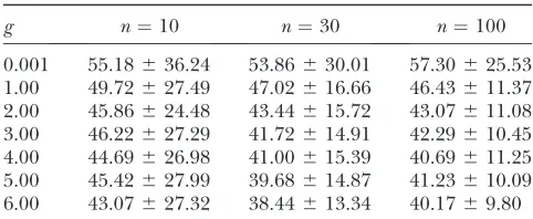
Performance of the LS statistic:Tables 1 and 2 show
the performance of the LS method in estimatinggandu
for the caseu¼40. In these tables the ‘‘size’’ of the table, in terms of increasingg, corresponds to the range of consistency for estimation of g. Thus, higher sample sizes generally gave better estimates ofg. Table 2 shows that simultaneous estimation of u is nearly unbiased over a wide range ofg—the reason being thatuappears in Equation 8 linearly. It is also shown that a significant reduction in MC standard deviation of the estimators can be achieved by increasing sample size. In all cases, the MC standard deviation of the estimators decreases with increased numbers of sequences. There is a slight bias in estimation near g ¼ 0.001 because of the singularity atg¼0 in Equation 2. As noted previously, however, one may use the UPBLUE method to estimate
uby Fu(1994a) at g¼0 (or at least its assumption of constant population size to compute the expected branch lengths in Equation 10).
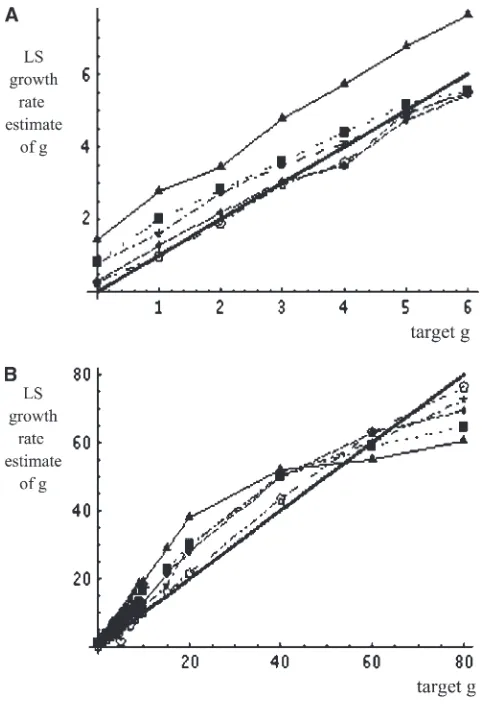
Figure 2 graphically shows the effect of sample size on the performance of LS estimation. For higher sub-stitution rate (u . 40), a significant range of growth rates can be consistently estimated. Better knowledge of the gene tree always allows expansion of the range of
consistent estimation. Figure 2A shows that for a range of g from 0.001 to 6, consistent estimation of g was possible for the unknown tree. Lack of knowledge of the actual gene tree significantly affects the ability to consistently estimateg.5 foru¼40. Figure 2B shows that the range of consistent estimation forgin the case
u¼40 is in the range ofgfrom 0.001 to 80 for the known gene tree. Since many rapid population expansions, such as for humans and viruses, may lie in this range it is important to correct the bias for any point estimates obtained that lie in this range. Below, I show how to address this problem using the jackknife bias-correction statistic. I then compare this statistic to those obtained using the more standard parametric bootstrap method.
Comparison of LS and ML statistics:In this section, I
compare the LS and ML statistics, utilizing the LS surface as a tool to diagnose performance. A ML surface should exhibit a maximum with respect to the mini-mum on the LS surface. Therefore, it is possible to investigate how the statistics behave by visually scanning the distribution of MC replicates around the LS mini-mum in (u,g) parameter space. I show that there are two scales in parameter space that determine the properties of the estimators. The first is determined by a ‘‘local’’ region surrounding a LS minimum point that deter-mines EVE estimates. This is determined by the LS criterion,i.e., the minimization of Equation 10. In this region, one would expect the distribution of MC replicates to cluster around the minimum, with density highest over the target parameters. In fact, a second ‘‘global’’ region over (u,g) parameter space plays a role with respect to the LS surface. This happens because of the appearance of a large plateau in parameter space. In this section I show how this plateau affects performance of the MLvs.the LS estimator.
Figure 3C shows the distribution of Monte Carlo replicates for the targetg¼5 andu¼60 at a sample size
n¼10. Figure 3, D–F, shows the distribution of Monte
TABLE 1 EVEgestimates
g n¼10 n¼30 n¼100
0.001 1.4162.98 0.8261.55 0.7861.15 1.00 2.7764.50 1.9862.23 1.6061.30 2.00 3.4464.69 2.8263.06 2.7261.93 3.00 4.7566.19 3.5963.06 3.4962.38 4.00 5.7466.63 4.3963.77 4.1062.65 5.00 6.7967.53 5.1764.21 4.9362.81 6.00 7.6568.73 5.5564.09 5.4963.04
The effect of varying sample size on consistency of growth rate estimation is shown. Estimates are means followed by standard deviations computed from 10,000 Monte Carlo rep-licates. Parameters used for simulating each replicate were
u¼ 40,m ¼0.001, andN0¼ 20,000. Variables are defined
asn(number of sequences),g(growth rate), andu¼2N0m.
TABLE 2 EVEu-estimates
g n¼10 n¼30 n¼100
0.001 55.18636.24 53.86630.01 57.30625.53 1.00 49.72627.49 47.02616.66 46.43611.37 2.00 45.86624.48 43.44615.72 43.07611.08 3.00 46.22627.29 41.72614.91 42.29610.45 4.00 44.69626.98 41.00615.39 40.69611.25 5.00 45.42627.99 39.68614.87 41.23610.09 6.00 43.07627.32 38.44613.34 40.1769.80
The effect of varying sample size on consistency of u -estimation across a range of growth rates is shown. Estimates shown are means followed by standard deviations computed from 10,000 Monte Carlo replicates. Parameters used for sim-ulating each replicate were u ¼ 40, m ¼ 0.001, and N0 ¼
Carlo replicates for the targetg¼15 andu¼60 at three different sample sizesn¼10, 30, and 100. For bothg¼5 andg¼15, the sample size ofn¼10 shows a cloud of LS and ML replicates close to the targets (see Figure 3, C and D). Also several outliers appear for both the LS and the ML estimates. However, the LS outliers appear to track the valley in the LS surface, while the ML estimators tend to be dispersed on a steeply rising ridge in the LS surface as shown in Figure 3A. The height of these ridges requires blowing up the region around the targets to see contours of the valley (see Figure 3B). FLUCTUATE outperforms EVE for the case shown in Figure 3C. It has a MC mean closer to the target than EVE, with smaller standard deviation. However, for the cases shown in Figure 3, D–F, the presence of outliers
shifts the mean MC value foruaway from its target. This gets progressively worse as the sample size increases— see Figure 3, E (n¼30) and F (n¼100). In contrast to the severe estimation bias observed foru, FLUCTUATE estimation ofgappears to be nearly unbiased. However, this conclusion must be accepted with the proviso that perfect knowledge of u0 ¼2N0m is available. Table 3 gives the MC means and standard deviation for the comparison between LS and ML statistics.
For larger sample sizes the distributions of the ML and LS estimates move further apart. Overall, these results imply that the ML estimator FLUCTUATE does not exhibit consistency at high growth rates and sample sizes when estimatingu. However, at small growth rate and small sample size FLUCTUATE outperforms EVE.
Previous MCMC studies for infinite-sites models (Wakeley et al.2001) have shown that the likelihood surface for changing population size has a complex topography: the parameters become nonidentifiable in some regions and plateaus appear. Beaumont (1999) made similar observations with likelihood modeling of microsatellite data. The findings of this section lend support to this earlier work. Under rapid population expansion the majority of the mutations are in the terminal branches of the tree. In a population sample, this appears as a sequence with a common ancestral haplotype and with the remaining haplotypes appearing as singletons. Such a star-shaped coalescent tree gives rise to a difficult data set for an MCMC coalescent likelihood method. For these data the MCMC compu-tation may generate the same star-shaped pattern for many choices ofuand growth rate. Indeed, Stephens (1999) and Stephens and Donnelly (2000) have previously predicted such computational difficulties for certain classes of MCMC methods. They noted that some MCMC algorithms, such as FLUCTUATE, use a fixed or ‘‘driving’’ value ofu. This gives rise to the pos-sibility that such algorithms find modes in an essentially flat surface or ridge where none are present. Figure 3A shows a steeply rising LS contour up to a long flat plateau. The FLUCTUATE MC replicates project onto the contours of such a plateau (see Figure 3F). The large pink dot centered at the cloud of replicates suggests that it may be at the center of a mode ‘‘found’’ by FLUCTU-ATE where clearly none is present.
Effect of recombination on the LS statistic:
Schierup and Hein (2000a) demonstrated that even small amounts of recombination can produce biases in tree reconstruction. These biases can affect phylogenetic inferences using reconstructed trees for nucleotide se-quence data. For example, bias from recombination can cause trees to superficially resemble phylogenies for sequences from an exponentially growing population. They also found that recombination created a large overestimation of rate heterogeneity and that standard ML methods ½the DNAml and DNAmlk programs of PHYLIP (Felsenstein1995)could not infer the
pres-Figure 2.—Performance of least-squares statistics. Lines
are connected between computed mean estimates using 10,000 Monte Carlo replicates. Values used for simulating each replicate wereu¼40,m¼0.001,N0¼20,000. Sequence
length is 1000 nucleotides. Variables are defined as follows:n, number of sequences;l, number of loci;g, growth rate; and
u¼2N0m. The solid thick line represents unbiased
ence of a molecular clock from sequence data (Schierup and Hein 2000b). Given that the LS method uses the shape of a single phylogenetic tree to estimate parame-ters, I tested the LS estimator on several thousand simulated samples of nucleotide sequences exhibiting varying amounts of recombination. I used the coalescent
algorithm with recombination described in Hudson (1983), modified so as to include exponential population growth. Since the generation of the coalescence and recombination events are independent, I was able to use the approach described in this article to efficiently sim-ulate the coalescent time distribution under
recombina-Figure3.—Comparison of least-squares (EVE) and maximum-likelihood (FLUCTUATE) estimation of growth rate (g) andu.
tion (Fearnhead and Donnelly2001). The mutation model used was the Jukes–Cantor model (Li1997) and was applied to simulate nucleotide data sets under re-combination as described in the article by Schierupand Hein(2000a).
I examined the performance of estimation under two scenarios. First, if the growth rate is zero, how well will the LS estimator perform given varying rates of recombina-tion? Second, in an exponentially growing population with high growth rate, how well does the LS estimator perform under varying rates of recombination?
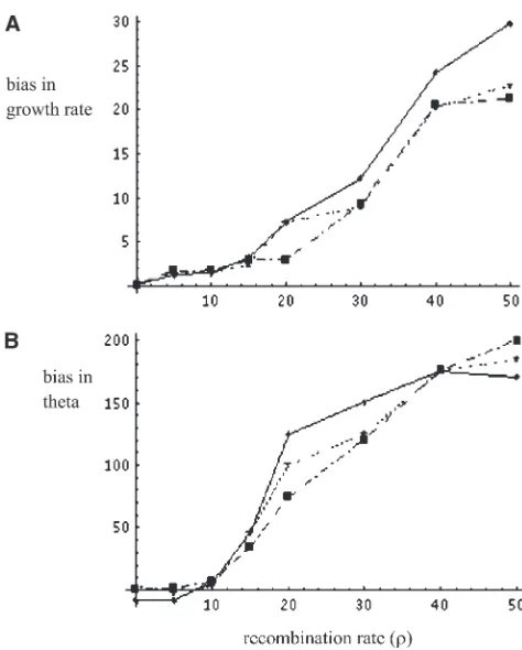
The results for the first case are shown in Figure 4. Setting the growth rate to zero in the simulations allows generating a null distribution on the estimators to determine the range of bias created by recombination. For low to moderate rates of recombination (r¼0–15) the LS estimator performs reasonably well. One ob-serves growth rates close to zero in each case. The range of estimation bias lies well within the range of that observed to be caused by intrinsic bias in the coalescent time distribution. Forr.15, however, the bias due to recombination gradually increases with the amount of recombination. Each point in Figure 4 was computed from the mean over 1000 replicated data sets.
For the second case I simulated samples of nucleotide sequences under moderate growth rate (g ¼15) and varying rates of recombinationr¼0–50. The results are shown in Figure 5. As in the previous case, in the region (r ¼ 0–15) the LS estimator appears to perform reasonably well. In this region the estimates ofgandu
exhibit low bias, on the order of that observed in the absence of recombination. Forr.15, the bias caused by recombination starts to increase the estimation bias of the observed estimate ofg, causing it to become more and more inflated. This bias appears to rise more rapidly in the presence of high growth than in the absence of growth (compare Figures 4 and 5). Each point in Figure 5 was computed from the mean over 1000 replicated data sets.
Inference on sample with parameters unknown: LS
statistics were computed for the African subset of the sampled human mtDNA sequenced by Vigilantet al. (1991). This gave the LS point estimates ðˆu;gˆÞ ¼ ð250;63:75Þ, which imply a significant recent popula-tion expansion (see Figure 6A). The distribupopula-tions of the MC replicates for all three simulation-based estimators
track the LS surface. This makes sense in light of the results shown earlier (see Tables 1 and 2, Figure 2) for the case when the target is known.
Consider next the quantification of estimation bias. Parametric bootstrap estimates of the point estimate were computed with the tree assumed unknown. The results for this are shown in Figure 6B. The mean is shown as the large dot at (u,g)¼(197.82639.35, 39.70 6 13.13), and the small blue dots correspond to MC replicates. Although extreme bias is present in this
Figure4.—Reliability of estimating (A) growth rate (g) and
(B) u under recombination. Each point represents an esti-mate of g ¼ 0 under a given level of recombination rate (r). The level of bias under recombination is about the same as expected as that produced by intrinsic bias in the coales-cent time distribution (see Tables 1 and 2 for estimates of g¼0.001 with no recombination) until the value ofr¼15 is reached. After this point a rapid increase in estimation bias is observed. Each point was computed using 1000 replicates at sample sizes 20, 50, and 100, denoted on the graphs by the star, triangle, and box symbols, respectively.
TABLE 3
Comparison between LS and ML statistics
n g EVEg FLUCTUATEg u EVEu FLUCTUATEu
10 5 10.24615.53 6.1163.88 60 79.88662.64 72.88662.00
10 15 11.2564.64 20.30615.44 60 55.10611.53 222.006768.40
50 15 9.7265.02 14.9865.78 60 49.36614.82 149.696923.37
estimator the spread of the replicates closely tracks the LS surface determined by the point estimate. Next parametric bootstraps were computed of the point estimate with the tree assumed known. The results are shown in Figure 6C. The MC mean is shown as the large dot at (u,g)¼(259.526 66.78, 69.88 6 30.25). This estimator shows substantially less bias. Finally, the non-parametric jackknife estimator gives a nearly unbiased estimate of the target. The small dots in Figure 6D are the MC jackknife replicates and these cluster tightly around the target. Although the estimated population growth rate for the African sample was very high it was still possible to obtain a nearly unbiased estimate of the point estimate using the jackknife.
The jackknifing statistic allows taking advantage of the intuitive idea that most of the mutations with information with regard to computing accurate esti-mates ofuandglie on the tips of the coalescent tree. Thus, jackknifing may be regarded as a computationally cheap way to take advantage of this property to obtain nearly unbiased estimates of the parameters. It is essentially a recalibration method that allows reweight-ing the estimator usreweight-ing the residuals of the nonlinear mutation model. The jackknifing is so efficient it
effectively weights each external branch as if it were adding genetic information from many independent loci (see Figure 2 for the casesn¼30,l¼10). However, in this case the only information in the sample is from a single locus—the human mtDNA.
DISCUSSION
In this article I show that it is possible to infer sources of bias with regard to coalescent estimation of a sample of sequences in an expanding population. Once the bias has been quantified, it is then possible to rapidly compute a bias-corrected estimator. In this section, I address two issues associated with these problems: LS estimation vs. ML estimation and the relationship between the results of this article and ongoing work in MCMC estimation methods.
Least-squaresvs.maximum-likelihood estimation:In
many situations a ML estimator is preferable over a LS estimator because the former is more flexible and can incorporate statistical tests more readily than the latter. However, estimation of demographic and selective parameters using the coalescent is an inherently non-linear problem. That is, the surface to be minimized or maximized is likely to have multiple optima and a complex topography. Estimating likelihoods when the tree is not known or approximated is extremely com-putationally intensive in determining this surface. De-spite this, using a parametric bootstrap it is possible to compare the ML and LS estimators. One generates Monte Carlo replicate data sets and superimposes the resulting estimates on top of each other. The LS estimates should cluster around the minimum and the ML should cluster around a maximum. The minima and the maxima should be approximately centered over each other. Thus the two clusters should lie roughly on top of each other with centers over the target. This is true for the LS estimator (EVE) but not always for the ML estimator analyzed in this article (FLUCTUATE). As sample size increases the correlation between optima located on the LS surface and optima located on the ML surface becomes lost. As sample size increases one would expect that an efficient estimator should become more accurate in predicting the target. My results show that the LS estimator does have a minimum over the target and becomes more accurate in predicting the target as sample size increases. I also show that the LS point estimator can be efficiently bias corrected if a nonparametric resampling estimation method is used.
Measurement error, summary statistics, and MCMC:
Recently Sisson (2007) pointed out some of the technical difficulties associated with developing MCMC algorithms for complex genetic data. He reviews com-putational problems associated with application of standard Metropolis–Hastings samplers to population genetics problems involving intractable likelihoods. As
Figure5.—Reliability of estimating (A) growth rate (g¼
15) and (B)u(¼60) under a given level of recombination (r), withn¼100. The level of bias under recombination is about the same as expected as that produced by intrinsic bias in the coalescent time distribution (see Tables 1 and 2 for es-timates ofg¼0.001 with no recombination) until the value of
noted above, Stephens(1999) earlier pointed to similar problems, specifically centered around integration of the Felsenstein equation (Heyand Nielsen2007). An important part of Sisson’s critique lies in evaluating how to construct proposals for MCMC algorithms on the basis of summary statistics that allow efficient ‘‘mixing’’ of the algorithm. He points to the analysis of Tanakaet al. (2006), who constructed a stochastic model at the genetic level that allows direct application of the Metropolis– Hastings approach of Marjoramet al.(2003) to a sum-mary statistic. Such an approach is related to the methods developed in the present article. However, the method would have been substantially slower and I would never have been quite sure when to stop the algorithm. Instead I implemented a cheaper LS model that allowed obtaining a fast answer. The frequentist framework developed here can be expressed within the framework of Bayesian sensitivity analysis (Oakleyand O’Hagan 2004). Whatever framework one chooses, however, the present article offers up a cheap and fast method of obtaining parameter estimates for complex genetic data sets that can be compared to
computation-ally expensive MCMC methods. Future work should lie in bringing together these two approaches into a more complete and useful statistical theory of genomic data.
I thank the associate editor, two anonymous reviewers, Romulus Breban, Gordon Harkins, and Paul Schliekelman for their work on helping me to improve the overall presentation and quality of the manuscript. This work was partly supported by grants from the National Institutes of Health (R01 HD34350-01A1) to Keith A. Crandall and (R29 GM50428) to Y.-X. Fu.
LITERATURE CITED
Avise, J. C., 2000 Phylogeography: The History and Formation of Species.
Harvard University Press, Cambridge, MA.
Beaumont, M. A., 1999 Detecting population expansion and
de-cline using microsatellites. Genetics153:2013–2029.
Cabrera, J., and L. T. Fernholz, 1999 Target estimation for bias
and mean square error reduction. Ann. Stat.27(3): 1080–1104. Crandall, K., D. Posadaand D. A. Vasco, 1999 Effective
popula-tion sizes: missing measures and missing concepts. Anim. Con-serv.2:317–319.
Christianini, N., and M. W. Hahn, 2007 Introduction to
Computa-tional Genomics.Cambridge University Press, Cambridge, UK. Deng, W.-H., and Y.-X. Fu, 1996 The effect of variable mutation rates
across sites on phylogenetic estimation of effective population size. Genetics144:1271–1281.
Figure 6.—Comparison
Efron, B., and R. J. Tibshirani, 1993 An Introduction to the Bootstrap
(Monographs on Statistics and Applied Probability 57). Chap-man & Hall, London.
Emerson, B. C., E. Paradisand C. Thebaud, 2001 Revealing the
demographic histories of species using DNA sequences. Trends Ecol. Evol.16(12): 707.
Fearnhead, P., and D. P. Donnelly, 2001 Estimating recombination
rates from population genetic data. Genetics159:1231–1241. Felsenstein, J., 1995 PHYLIP (Phylogeny Inference Package),
Ver-sion 3.572. University of Washington, Seattle.
Fu, Y.-X., 1994a A phylogenetic estimator of effective population size
or mutation rate. Genetics136:685–692.
Fu, Y.-X., 1994b Estimating effective population size or mutation
rate using the frequencies of mutations of various classes in a sample of DNA sequences. Genetics138:1375–1386.
Fu, Y.-X., 1995 Statistical properties of segregating sites. Theor.
Popul. Biol.48:172–197.
Fu, Y.-X., and W.-H. Li, 1999 Coalescing into the 21st century: an
overview and prospects of coalescent theory. Theor. Popul. Biol. 56:1–10.
Givens, G. H., and J. A. Hoeting, 2005 Computational Statistics.
Wiley-Interscience, Hoboken, NJ.
Gourieroux, C., and A. Monfort, 1996 Simulation-Based
Economet-ric Methods.Oxford University Press, Oxford.
Griffiths, R. C., and S. Tavare´, 1994 Sampling theory for neutral
alleles in a varying environment. Philos. Trans. R. Soc. Lond. B 344:403–410.
Hein, J., M. H. Schierupand C. Wiuf, 2005 Gene Genealogies,
Varia-tion and EvoluVaria-tion. A Primer in Coalescent Theory.Oxford University Press. Oxford.
Hey, J., and R. Nielsen, 2007 Integration with the Felsenstein
equa-tion for improved Markov chain Monte Carlo methods in popu-lation genetics. Proc. Natl. Acad. Sci. USA104:2785–2790. Hickerson, M. J., G. Dolmanand C. Moritz, 2006 Comparative
phylogeographic summary statistics for testing simultaneous vi-cariance. Mol. Ecol.15:209.
Hjorth, J. S. U., 1994 Computer Intensive Statistical Methods: Validation
Model Selection and Bootstrap.Chapman & Hall, London. Hudson, R. R., 1983 Properties of a neutral allele model with
intra-genic recombination. Theor. Popul. Biol.23:183–201. Hudson, R. R., 1990 Gene genealogies and the coalescent process,
pp. 1–44 inOxford Surveys in Evolutionary Biology, edited by P. H. Harveyand L. Partridge. Oxford University Press, London/
New York/Oxford.
Kimura, M., 1983 The Neutral Theory of Molecular Evolution.
Cam-bridge University Press, CamCam-bridge, UK.
Knowles, L. L., 2004 The burgeoning field of statistical
phylogeog-raphy. J. Evol. Biol.17:1–10.
Kuhner, M. K., J. Yamotoand J. Felsenstein, 1995 Estimating
effective population size and mutation rate from sequence data using Metropolis-Hastings sampling. Genetics140:1421– 1430.
Kuhner, M. K., J. Yamotoand J. Felsenstein, 1998 Maximum
like-lihood estimation of population growth rates based on the coa-lescent. Genetics149:429.
Li, W.-H., 1997 Molecular Evolution.Sinauer Associates, Sunderland,
MA.
Li, W.-H., and Y.-X. Fu, 1994 Estimation of population parameters
and detection of natural selection from DNA sequences, pp. 112–125 inNon-Neutral Evolution: Theories and Molecular Data, edi-ted by B. Golding. Chapman & Hall, London.
Marjoram, P., and S. Tavare´, 2006 Modern computational
ap-proaches for analyzing molecular genetic variation data. Nat. Rev. Genet.7:759–770.
McVean, G., and C. C. A. Spencer, 2006 Scanning the human
ge-nome for signals of selection. Curr. Opin. Genet. Dev.16:624– 629.
Nielsen, R., S. Williamson, Y. Kim, M. J. Hubisz, A. G. Clarket al.,
2005 Genomic scans for selective sweeps using SNP data.
Genome Res.15:1566–1575.
Oakley, J. E., and A. O’Hagan, 2004 Probabilistic sensitivity
analy-sis of complex models: a Bayesian approach. J. R. Stat. Soc. B 66(3): 751–769.
Quenouille, M. H., 1956 Notes on bias in estimation. Biometrika 43:353–360.
Rogers, A. R., and H. Harpending, 1993 Population growth makes
waves in the distribution of pairwise genetic differences. Mol. Biol. Evol.9:552–569.
Schaffner, S., C. Foo, S. Gabriel, D. Reich, M. J. Daly et al.,
2005 Calibrating a coalescent simulation of human genome se-quence variation. Genome Res.15:1576–1583.
Schierup, M., and J. Hein, 2000a Consequences of recombination
on traditional phylogenetic analysis. Genetics156:879–891. Schierup, M., and J. Hein, 2000b Recombination and the
molecu-lar clock. Mol. Biol. Evol.17:1578–1579.
Shao, J., and D. Tu, 1995 The Jackknife and the Bootstrap.
Springer-Verlag, New York.
Sisson, S. A., 2007 Genetics and stochastic simulation do mix! Am.
Stat.61(2): 112–119.
Slatkin, M., and R. R. Hudson, 1991 Pairwise comparisons of
mi-tochondrial DNA sequences in stable and exponentially growing populations. Genetics129:555–562.
Stephens, M., 1999 Problems with computational methods in
pop-ulation genetics. Bulletin of the 52nd Session of the Interna-tional Statistical Institute, Helsinki.
Stephens, M., and P. Donnelly, 2000 Inference in molecular
pop-ulation genetics. J. R. Stat. Soc. B62:605–635.
Swofford, D. L., and G. J. Olsen, 1990 Phylogenetic
reconstruc-tion, pp. 411–501 inMolecular Systematics, edited by D. M. Hillis
and C. Moritz. Sinauer Associates, Sunderland, MA.
Tajima, F., 1983 Evolutionary relationship of DNA sequences in
fi-nite populations. Genetics105:437–460.
Tajima, F., 1989 The effect of change in population size on DNA
polymorphism. Genetics123:597–601.
Tanaka, M. M., A. R. Francis, F. Luciani and S. A. Sisson,
2006 Estimating tuberculosis transmission parameters from ge-notype data using approximate Bayesian computation. Genetics 173:1511–1520.
Wakeley, J., R. Nielsen, S. N. Liu-Cordero and K. Ardlie,
2001 The discovery of single-nucleotide polymorphisms—
inferences about human demographic history. Am. J. Hum. Genet.60:1332–1347.
Watterson, G. A., 1975 On the number of segregating sites in
ge-netic models without recombination. Theor. Popul. Biol.7:256– 276.
Vasco, D. A., K. A. Crandalland Y.-X. Fu, 2001 Molecular
popula-tion genetics: coalescent methods based on summary statistics, pp. 173–216 inComputational and Evolutionary Analysis of HIV Mo-lecular Sequences, edited by A. G. Rodrigoand G. H. Learn, Jr.
Kluwer Academic Publishers, Dordrecht, The Netherlands. Vigilant, L. M., M. Stoneking, H. Harpending, K. Hawkesand
A. C. Wilson, 1991 African populations and the evolution of
human mtDNA. Science253:1503–1507.