A New Index Calculus Algorithm for the
Elliptic Curve Discrete Logarithm Problem
and Summation Polynomial Evaluation
Gary McGuire
∗Daniela Mueller
†School of Mathematics and Statistics
University College Dublin
Ireland
Abstract
The introduction of summation polynomials for elliptic curves by Semaev has opened up new avenues of investigation in index calcu-lus type algorithms for the elliptic curve discrete logarithm problem, and several recent papers have explored their use. We propose an in-dex calculus algorithm to solve the Elliptic Curve Discrete Logarithm Problem that makes use of a technique for fast evaluation of the sum-mation polynomials, and unlike all other algorithms using sumsum-mation polynomials, does not involve a Gr¨obner basis computation. We fur-ther propose anofur-ther algorithm that does not involve Gr¨obner basis computations or summation polynomials. We give a complexity esti-mate of our algorithms and provide extensive computational data.
Keywords
elliptic curves, ECDLP, index calculus, summation polynomials.
∗Research supported by Science Foundation Ireland Grant 13/IA/1914.
†Research supported by a Postgraduate Government of Ireland Scholarship from the
1
Introduction
Let E be an elliptic curve over a finite field Fq, where q is a prime power.
In practice, q is often a prime number or a large power of 2. Let P and Q
be points on E. The Elliptic Curve Discrete Logarithm Problem (ECDLP) is finding an integer l (if it exists) such that Q=lP. The integer l is called the discrete logarithm of Q to baseP.
The ECDLP is a hard problem that underlies many cryptographic schemes and is thus an area of active research. The introduction of summation poly-nomials by [Sem04] has led to algorithms that resemble the index calculus algorithm of the DLP over finite fields. We outline how the algorithm works in general first.
LetG be a cyclic group with given generatorg. We wish to find the discrete logarithm of a target element hto the base g. A sketch of the index calculus algorithm for G is the following.
1. Factor Base step. Define a subsetF ⊆G, called the factor base. 2. Relation step. Collect linear relations involving factor base elements.
3. Linear Algebra step. Combine and solve relations using linear alge-bra.
4. Solving step. Use the results to find the discrete logarithm of the target element h.
When the group G is the multiplicative group of a finite field, typically the first three steps do not depend on the target element. Steps 1-3 will result in the logs of the factor base elements, and only in the final step will the target element be used, when its log will be calculated. This is different from typical index calculus algorithms for the ECDLP, where the relations in Step 2 depend on the target element, although the choice of factor base in Step 1 does not (see section 2.2). In the algorithms under discussion in this paper, the choice of factor base in Step 1 does depend on the target element.
It is also not a priori clear how to find relations in Step 2. Summation polynomials enable a decomposition over the factor base in certain cases for elliptic curves, and we give their definition in section 2.1. Section 2.2 shows how this decomposition can be achieved for certain choices of factor base.
Most papers have focused on elliptic curves over an extension field Fqn, and
use subfields in the algorithm, see for example [Gau09], [FHJ+14], [JV13]. The case of elliptic curves over prime order fields seems to be much harder to tackle. Our algorithms in this paper are aimed at prime order fields, although they are valid for any finite field. In section 2.3, we give a brief overview of the different approaches to the prime field case using summation polynomials. A recent paper by Amadori-Pintore-Sala [APS18] published inFinite Fields and their Applications has shown how to simplify these algorithms to avoid the linear algebra step and reduce the number of Gr¨obner basis computations. We summarize their algorithm (as Algorithm 2.5) in section 2.3.
In section 3 we develop the algorithm in [APS18] to a new algorithm (Algo-rithm 3.1) which, unlike all other algo(Algo-rithms using summation polynomials, does not involve a Gr¨obner basis computation. This leads to a significant speedup over the other prime field algorithms.
In section 4 we then further develop our Algorithm 3.1 to Algorithm 4.1 which does not use summation polynomials at all, as well as not using Gr¨obner bases and not using a linear algebra step. This algorithm is fastest among all the algorithms discussed here, both in practice and in complexity.
In Section 5 we develop a method for fast evaluation of the summation poly-nomials. This improves the algorithms and allows us to evaluate summation polynomials S9 and S10 even though we cannot calculate the polynomials.
Section 6 contains an estimate of the complexity of the algorithm in [APS18], as well as a complexity estimate of our two algorithms presented here. Note that [APS18] did not contain an estimate of the complexity, indeed the au-thors state that they are “unable to estimate the complexity of solving our polynomial equation systems.” We will see that Algorithm 4.1 is best, fol-lowed by Algorithm 3.1 and last comes Algorithm 2.5. The algorithms have exponential complexity, which one would expect with a randomly chosen fac-tor base. Our analysis shows that all these algorithms are worse than the well known square-root algorithms such as Pollard-Rho. Nevertheless, we claim that Algorithm 4.1 is the best index calculus algorithm for prime order fields at the present time.
2
Background
2.1
Summation Polynomials
Definition 2.1: [Sem04] Let E be an elliptic curve over a field K. For
n ≥ 2, we define the summation polynomial Sn = Sn(X1, X2, . . . , Xn) of E
by the following property. Letx1, x2, . . . , xn ∈K, thenSn(x1, x2, . . . , xn) = 0
if and only if there exist y1, y2, . . . , yn ∈ K such that (xi, yi) ∈ E(K) and
(x1, y1) + (x2, y2) +. . .+ (xn, yn) = O, where O is the identity element ofE.
Semaev showed in [Sem04] how to compute the summation polynomials for elliptic curves in Weierstrass form:
Theorem 2.2: LetE be an elliptic curve given by Y2 =X3+AX+B over
a field K with characteristic 6= 2,3. Then the summation polynomials are given by
S2(X1, X2) = X1−X2,
S3(X1, X2, X3) = (X1−X2)2X32−2((X1+X2)(X1X2+A)+2B)X3+((X1X2−
A)2−4B(X1+X2)),
Sn(X1, . . . , Xn) = ResX(Sn−k(X1. . . , Xn−k−1, X), Sk+2(Xn−k. . . , Xn, X)) for
n ≥4 and any 1≤k ≤n−3.
Furthermore, the polynomials Sn, n ≥ 3, are symmetric, of degree 2n−2 in
each variable, of total degree (n−1)2n−2, and absolutely irreducible.
For more detail and for other characteristics, see [Sem04].
2.2
Point Decomposition with Summation
Polynomi-als
The following is a more detailed version of the index calculus algorithm as normally used for elliptic curves, see [Gau09] for example. We include it for comparison with our algorithms developed in this paper.
Definition 2.3: (Index Calculus) Let G be a cyclic group of points on an elliptic curve defined over Fq (here we use additive notation), let P be a
1. Factor Base step. Define a subsetF ⊆G, called the factor base. 2. Relation step. Collect relations that decompose over the factor base:
Let R =aP +bQ (a, b random integers), and try to write R as a sum of factor base elements, R =P1 +...+Pm, with P1, ..., Pm ∈ F. Store
the relations in matrix and vector format.
3. Linear Algebra step. Perform linear algebra on the matrix-vector equation to get an equation of the form αP +βQ= 0.
4. Solving step. If β is invertible modulo the group order r, then the discrete logarithm of Qis −α/β modr.
Let F = {P1, P2, . . . , Ps} be the factor base of points on E, where s = |F |
is the size of the factor base. Let r1, r2 be random integers and let R =
r1P+r2Q. In order to writeR =P1+...+Pm, withP1, ..., Pm ∈ F, we use the
(m+ 1)th summation polynomial: writingR= (x
R, yR), we try to find a
solu-tion (x1, . . . , xm) of Sm+1(X1, . . . , Xm, xR) = 0 such that ∃ yi with (xi, yi)∈
F, 1≤i≤m. Then∃εi =±1 such thatε1(x1, y1)+. . .+εm(xm, ym)±R =O.
Once we have found at leasts+ 1 independent relations of this form, we can find logP(Q) by solving the matrix equation
ε1,1 . . . ε1,s
ε2,1 . . . ε2,s
. . .
εs+1,1 . . . εs+1,s
logP(P1)
logP(P2)
. . .
logP(Ps)
=
r1,1
r2,1
. . . rs+1,1
+
r1,2
r2,2
. . . rs+1,2
logP(Q)
where εi,j ∈ {0,1,−1}, 1≤i≤s+ 1, 1≤j ≤s.
Gaudry suggests in [Gau09] a way to solve Sn+1(X1, . . . , Xn, xR) = 0, if
E is defined over Fqn = Fq[t]/f(t), q a prime power, f irreducible of
de-gree n. He defines the factor base to be all points with x-coordinate in Fq,
F = {(x, y) ∈ E(Fqn) : x ∈ Fq}. Note that we only need to include one of
{(x, y),(x,−y)} in the factor base if we allow coefficients ±1 in the decom-position of R. Now writing Sn+1(X1, . . . , Xn, xR) =
Pn−1
i=0 ϕi(X1, . . . , Xn)ti,
we instead solve ϕi(X1, . . . , Xn) = 0 over Fq, 0 ≤ i ≤ n −1, obtaining a
2.3
Factor base over prime fields
If the elliptic curve is defined over a prime field (Fp for p a prime number)
Semaev suggests in [Sem04] to define the factor base to be all points with ”small” x-coordinate (taking the finite field elements to lie in the interval [0, ..., p−1] and treating them as integers in order to bound them). However, nobody knows how to find these small points efficiently.
Petit et al. showed in [PKM16] how to define the factor base as points on the curve with x-coordinate a solution of the composition of some small-degree rational maps. The decompositions are then found by solving the polyno-mial system obtained from these rational maps and summation polynopolyno-mials. Their approach seems to be the first working case for curves defined over prime fields, but it is only feasible for small parameters. (The largest field in their experiments is F4206593 and one Gr¨obner basis computation takes
4975.07 sec. Compare this with our results in section 7: the largest field in our experiments is F30951732491 and the total time to solve the ECDLP is
6850.10 sec.)
Amadori-Pintore-Sala [APS18] showed a different way of defining the factor base that enabled them to significantly reduce the number of polynomial sys-tems that need to be solved, and also avoid the linear algebra step, leading to an improvement in the running time. We will explain their approach now and give a complexity estimate in section 6.
Step 1. Lets be the desired size of the factor base (we will show later how to select s). Compute random integers a1, ..., as, b1, ..., bs. Then the factor base
F is all points {a1P +b1Q, ..., asP +bsQ}.
Step 2. Find a relation of the form P1+. . .+Pm =O with Pi ∈ F.
Step 3. Substitute each Pi with the corresponding aiP +biQ and get the
relation
m
X
i=1
aiP + m
X
i=1
biQ=O. (1)
Then Q = −Pm
i=1(ai/bi)P provided
Pm
i=1bi is invertible modulo the order
of E (if Pm
i=1bi is not invertible, start again). We have thus solved for the
Remark 2.4: Note that the factor base is chosen randomly, as opposed to the methods mentioned in the first two paragraphs of this section. The al-gorithm may fail, and if so then it is run again and the re-run will involve a different choice of random factor base. This is in contrast to the other meth-ods, where the factor base is clearly defined, and re-running the algorithm does not result in a different factor base.
In step 2, Amadori et al. propose the following system of polynomial equa-tions to find relaequa-tions. Let V be the set of x-coordinates of all the points in the factor base, i.e. V = {x|(x, y) ∈ F }. Let f(x) = Q
v∈V(x−v). Then
they solve (via Gr¨obner basis algorithms) the system
Sm(X1, . . . , Xm) = 0
f(X1) = 0 (2)
. . .
f(Xm) = 0.
Hence, they only consider solutions to Sm(X1, . . . , Xm) = 0 of the form
(x1, ..., xm)∈Vm, i.e. corresponding to points in the factor base.
Since f has degree s, which is the size of the factor base and could be quite large, the resolution of the system could be slow. So they propose instead usingmdifferent polynomials, by partitioning the factor base intomdifferent factor bases Fi of more or less equal size ms. V is partitioned into m sets Vi
accordingly, giving m polynomials fi(x) =
Q
v∈Vi(x−v). They then solve
the system
Sm(X1, . . . , Xm) = 0
f1(X1) = 0 (3)
. . .
fm(Xm) = 0.
Now each of the fi only has degree ms approximately, and therefore the
For completeness, we give the full algorithm from [APS18] with this approach:
Algorithm 2.5: [APS18]
Input: elliptic curve E overFp, points P and QonE, integers m, s,
summa-tion polynomial Sm
Output: logP(Q)
1. Letsbe the size of the factor base. Compute random integersa1, ..., as,
b1, ..., bs. The factor base F is all points {a1P +b1Q, ..., asP +bsQ}.
The corresponding set containing only the x-coordinates of the factor base points is V ={x|(x, y) ∈ F }. Partition this set intom sets Vi of
approximately equal size. Let fi(x) =
Q
v∈Vi(x−v), i= 1, . . . , m.
2. Using a Gr¨obner basis algorithm, solve system (3). If there is no solu-tion, go back to step 1.
3. If{x1, . . . , xm}is a solution to the above system, then each xi ∈Vi and
there existyisuch that (x1, y1)+. . .+(xm, ym) = Owhere either (xi, yi)
or−(xi, yi) are inF. Substituting each±(xi, yi) with the corresponding
±(aiP+biQ), we get a relation of the form
Pm
i=1±aiP+
Pm
i=1±biQ=O
and can solve for the discrete logarithm of Q, provided Pm
i=1±bi is
invertible modulo the order of E.
3
Avoiding Gr¨
obner basis computations and
Linear Algebra step
While systems (2) and (3) are a way of algebraically describing that the so-lutions to Sm lie in the factor base, it seems to us that there should be a
better way to solve this problem than feeding the polynomial system into a Gr¨obner basis algorithm. This approach essentially treats the polynomialsfi
(or f) as input polynomials to find their common roots withSm even though
we already know their complete factorisation.
Algorithm 3.1:
Input: elliptic curve E overFp, points P and QonE, integers m, s,
summa-tion polynomial Sm
Output: logP(Q)
1. Letsbe the size of the factor base. Compute random integersa1, ..., as,
b1, ..., bs. The factor base F consists of all points {a1P+b1Q, ..., asP+
bsQ}. The corresponding set containing only the x-coordinates of the
factor base points is denoted V ={x|(x, y)∈ F }.
2. Choose {x1, . . . , xm} a multiset of size m with each xi ∈ V and check
if Sm(x1, . . . , xm) = 0. If not, repeat with another multiset.
If Sm is non-zero for all multisets of size m, go back to step 1.
3. If Sm(x1, . . . , xm) = 0 for some {x1, . . . , xm}, then there exist yi such
that (x1, y1) +. . .+ (xm, ym) = O where either (xi, yi) or−(xi, yi) are
inF. Substituting each±(xi, yi) with the corresponding±(aiP+biQ),
we get (as in (1)) a relation of the form Pm
i=1±aiP +
Pm
i=1±biQ=O
and can solve for the discrete logarithm of Q, provided Pm
i=1±bi is
invertible modulo the order of E.
We will show later in Lemma 5.1 how to efficiently evaluate the summation polynomials Sm in step 2.
Remark 3.2: In step 2, we can alternatively choose a multiset of m points
{P1, . . . , Pm} from the factor base, and sum those points to see if they give
the point at infinity. This avoids using summation polynomials, and is in fact faster in theory and in practice (see section 6 and section 7). We omit the details for this algorithm. We refine this idea in the next section, and obtain an even faster algorithm.
4
Avoiding Summation Polynomials and
Gr¨
obner bases and Linear Algebra step
Algorithm 4.1:
Input: elliptic curve E overFp, points P and Qon E, integers m, s
Output: logP(Q)
1. Letsbe the size of the factor base. Compute random integersa1, ..., as,
b1, ..., bs. The factor base F is {a1P +b1Q, ..., asP +bsQ}.
2. Choose {P1, . . . , Pm−1} a multiset of size m −1 with each Pi ∈ F.
Choose v ∈Fm−1
2 , and let Pv = (−1)v1P1+. . .+ (−1)vm−1Pm−1. Check
if Pv ∈ F.
If Pv ∈ F/ for all v ∈Fm2−1, repeat with another multiset.
If there is no solution for all multisets of size m−1, go back to step 1.
3. If Pv ∈ F for some v then let Pm = −Pv and we get the relation
(−1)v1P
1+. . .+ (−1)vm−1Pm−1+Pm =O. Substituting each±Pi with
the corresponding±(aiP+biQ), we get (as in (1)) a relation of the form
Pm
i=1±aiP +
Pm
i=1±biQ=O and can solve for the discrete logarithm
of Q, provided Pm
i=1±bi is invertible modulo the order of E.
We will provide a complexity estimate of all algorithms in section 6.
Remark 4.2: The motivation for the three given algorithms was the ECDLP over prime fields. However, none of the algorithms require the field to be of prime order. They all work for any finite field.
Remark 4.3: Algorithm 2.5 and Algorithm 3.1 use summation polynomi-als, and therefore the input value of m must be ≤ 8 because the largest summation polynomial that has been computed so far is S8 as far as we are
aware (see [FHJ+14]). Algorithm 4.1 does not suffer from this problem, and
larger values of m can readily be used.
5
Summation Polynomial Evaluation
Next we will discuss a method for evaluating a summation polynomial Sm
which is faster than a straightforward brute force evaluation. For m = 3 there is no difference, so in our experiments with S3 we did not need to
The notation ms in this paper means that m is constant and small, and
s is arbitrarily large. In practice m is at most 10. We have in mind that
s =p1/m, as used in previous papers.
Lemma 5.1: EvaluatingSmat a point (x1, . . . , xm) can be done inO(log2p)
steps for m p.
Proof: It follows from the statement of Theorem 2.2 thatS3 can be evaluated
using at most 8 multiplications and 11 additions, and thus has complexity 8O(log2p) + 11O(logp).
For larger m, we make heavy use of the fact that
Res(f(a, X), g(a, X)) = ResX(f, g)(a)
for polynomialsf(x, y), g(x, y) whenever the leading coefficients are non-zero. Write S3(x1, x2, X) = a2X2+a1X+a0 and S3(x3, x4, X) = b2X2+b1X+b0.
By Theorem 2.2,
S4(x1, x2, x3, x4) = ResX(S3(x1, x2, X), S3(x3, x4, X))
= det
a2 a1 a0 0
0 a2 a1 a0
b2 b1 b0 0
0 b2 b1 b0
=a2(b0(a2b0−2a0b2−a1b1) +a0b21)
+b2(a1(a1b0−a0b1) +a20b2).
Using our optimisation for S3 to evaluate the ai and bi, we can evaluate S4
with at most 21 multiplications and 24 additions, and thus with complexity 21O(log2p) + 24O(logp).
For m≥5, again by Theorem 2.2,
Sm(x1, . . . , xm) = ResX(S3(x1, x2, X), Sm−1(x3, . . . , xm, X))
= det
a2 a1 a0 0 0 . . . 0
0 a2 a1 a0 0 . . . 0
. . .
b2m−3 b2m−3−1 . . . b0 0
0 b2m−3 . . . b1 b0
=a2(a2C12−a1C13+a0(C14−C23))
+a1(a1C23−a0C24) +a20C34
where Sm−1(x3, . . . , xm, X) = b2m−3X2
m−3
+b2m−3−1X2
m−3−1
matrix (Sylvester matrix ofS3andSm−1) with theithandjthcolumn removed
and the first and second row removed.
We can evaluate this expression with at most nine multiplications, six ad-ditions, and six determinant computations of 2m−3 by 2m−3 matrices. Also, we can evaluate the bi by m −4 recursive calls to this algorithm (m −4
calls because once we reach S4, we can evaluate it directly using the
ex-pression earlier in the proof). Thus, we can evaluate Sm using a total of
8(m−4) + 21 + 9(m−4) multiplications, 11(m−4) + 24 + 6(m−4) additions, and six determinant computations of matrices of size 2m−3 by 2m−3, six of size 2m−4 by 2m−4, . . ., and six of size 22 by 22.
We assume that the complexity of computing the determinant of an n by
n matrix is O(n3) (see [vzGG13], although this can be improved, see e.g. [KV05]). This gives a total complexity of (17m −47)O(log2p) + (17m −
44)O(logp) + 6(O(23(m−3)) +O(23(m−4)) +. . .+O(23·2)).
So far, the proof holds for any m. Finally, we assume m p and we get a
complexity of O(log2p) for evaluating Sm.
Remark 5.2: See math.ie/ecdlp/ecdlp.html for a Magma implementa-tion of the method described in this proof. In particular for m ≥ 4 it is significantly faster than first computing Sm and then evaluating it with
Magma’s in built evaluation function. This method even allows us to evalu-ate S9 and S10, although nobody has actually computed them yet as far as
we know.
6
Complexity Estimates
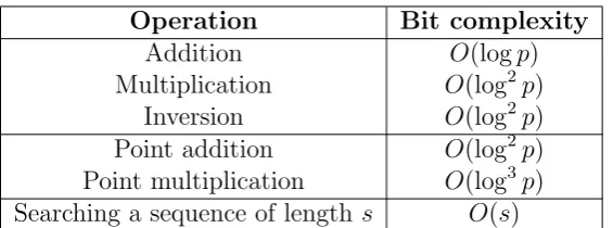
Table 1 summarises the complexity of operations inFpobtained from [MvOV96]
and of operations on an elliptic curve over Fp from [Sil09]. Please note that
Operation Bit complexity
Addition O(logp)
Multiplication O(log2p)
Inversion O(log2p)
Point addition O(log2p)
Point multiplication O(log3p)
Searching a sequence of lengths O(s)
Table 1: Bit complexity of basic operations in Fp and on an elliptic curve
over Fp (not best possible).
Remark 6.1: The number of ways of choosing m elements from a set of size s, allowing repetitions, is s+mm−1 which is approximately smm! forms. Relations can be of the form P1 ±. . .±Pm = O with Pi ∈ F, so we get
approximately 2m−m1!sm possibilities. The number of points on the curve is approximately p. Therefore, the probability of obtaining a relation of length
m inF is approximately 2mp−·m1s!m, wheres =|F | and ms.
Remark 6.2: There are ms ways of choosing each point in the relation giving 2m−1(s
m)
mpossibilities for relations of the formP
1±. . .±Pm =Owith eachPi
coming from the factor base partitionFiof size ms. Therefore, the probability
of obtaining a relation of length m with each point coming from a different partition of the factor base of size ms is 2mp·−m1msm.
Remark 6.3: The complexity of computing a factor base of sizesis bounded by O(slog3p), as can be seen from Table 1. (We have to do 2s point multi-plications of O(log3p) and s point additions of O(log2p).)
Remark 6.4: We would like the probability of finding a relation in the fac-tor base to be close to 1, i.e. in the case of Remark 6.2, we want 2m−1sm
mm ≈p,
so we should choose the factor base sizes accordingly. However, the authors of [APS18] propose s = p1/m as was chosen in other papers, e.g. [Gau09]. With this choice we will have to run (steps 1 and 2 of) Algorithm 2.5 an expected number of 2mmm−1 times. Therefore, even though we only require the
one as is claimed in [APS18].
The following result estimates the complexity ofone Gr¨obner basis computa-tion. Let ω ≤3 be the linear algebra constant (the constant in the exponent of the complexity of multiplying matrices, see Chapter 12 of [vzGG13]). The notation m s in this paper means that m is constant and small, and s is arbitrarily large.
Heuristic Result 6.5: The complexity of computing a Gr¨obner basis of system (3) in graded reverse lexicographical order is bounded by O(pω−ω/m) for s=p1/m and ms.
Proof: Let D be the maximum degree reached during a Gr¨obner basis com-putation. There are NN+D monomials of degree at most D in N variables, therefore the complexity of a Gr¨obner basis computation in graded reverse lexicographical order can be bounded by NN+Dω as the linear algebra is the most costly part of the algorithms (see [MP15] and [JV11]).
The maximum degreeDreached during a Gr¨obner basis computation can be bounded by the Macaulay bound (see [Laz83]) D≤Pl
i=1(di−1) + 1, where
l is the number of polynomials and di is the degree of the ith polynomial.
(Refer to [CG17] for a more detailed discussion.) As system (3) has m+ 1 polynomials in m variables, D can be bounded by Pm+1
i=1 (di−1) + 1. Also,
Sm has total degree (m−1)·2m−2 (Theorem 2.2) and each fi has degree
about ms. So we get
D≤(m−1)·2m−2−1 +m(s
m −1) + 1 = (m−1)·2
m−2
+s−m.
Thus,
N +D N
≤
m+ (m−1)·2m−2+s−m
m
= (s+ (m−1)·2
m−2)!
m!(s+ (m−1)·2m−2 −m)!
=(s+ (m−1)·2
m−2). . .(s+ (m−1)·2m−2−m+ 1)
m! .
There are m − 1 factors in the numerator, each dominated by s. So we approximate NN+D by smm−!1. Thus,
N +Dω
Heuristic Result 6.6: The complexity of Algorithm 2.5 is bounded by
mm
2m−1(O(p
1/mlog3p) +O(pω−ω/m))≈O(pω−ω/m)
for s=p1/m and ms.
Proof: Steps 1 and 2 of Algorithm 2.5 may have to be computed 2mmm−1 times,
each time with complexity O(p1/mlog3p) + O(pω−ω/m) by Remark 6.3 and
Heuristic Result 6.5. Once we get a factor base that yields a solution, we need to compute the solutions from the Gr¨obner basis in grevlex order. In theory, one may have to do a change of ordering algorithm to get a Gr¨obner basis in lexicographical ordering, from which we can compute the solutions. However, the probability of getting more than one solution to system (3) is negligible (by Remark 6.2, the probability of obtaining a relation of length
m is 2mmm−1 so the probability of obtaining two relations is the square of this).
When we only find one solution the Gr¨obner basis elements have the form
xi−a and therefore the change of ordering is trivial.
Remark 6.7: Even if the algorithm does find a grevlex Gr¨obner basis with two solutions, the basis elements will be quadratic or linear, and again this is easy to solve and a change of ordering is not necessary.
Remark 6.8: It is reasonable to assume that m is small when using sum-mation polynomials, since the largest sumsum-mation polynomial that has been computed so far is S8 (see [FHJ+14]).
Remark 6.9: With ω = 3 and m = 3 the complexity of Algorithm 2.5 is
O(p2). This roughly agrees with our experiments.
Heuristic Result 6.10: The complexity of Algorithm 3.1 is O(plog2p) for
m s and mp and smm−!1 ≥logp.
Proof: As noted in Remark 6.1, there are sm
m! ways of choosing m elements
from the set F of size s, allowing repetitions, for small m. By Lemma 5.1, evaluating Sm is O(log2p), giving a total of s
m
m!O(log 2
p) in the worst case. By Remark 6.1 we need an expected number of 2mp−·m1s!m trials, giving
p·m! 2m−1sm(
sm m!O(log
2
p) +O(slog3p))≈O(plog2p)
when sm−1
m! ≥logp.
Remark 6.11: Replacing the evaluation ofSm by addingm points together
Heuristic Result 6.12: The complexity of Algorithm 4.1 isO(p) forms
and s ≥(m−2) log2p.
Proof: There are 2m−1 sm−1
(m−1)! different ways of forming the sum ±P1±. . .±
Pm−1, with Pi ∈ F, allowing repetitions, for small m and s = |F |. Let
Pm = ±P1 ±. . .±Pm−1. The complexity of each sum is (m−2)O(log2p).
For each combination, we check if Pm is in F, which is O(s). If the sum is
in F, we get a relation of the form ±P1±. . .±Pm−1−Pm =O. So we still
get a relation with probability as in Remark 6.1, so the complexity of this algorithm is 2mp−·m1s!m(2m
−1 sm−1
(m−1)!((m−2)O(log
2p) +O(s)) +O(slog3p)). If
s ≥(m−2) log2p then this is p·smO(s)≈O(p) for smallm.
7
Experimental Results
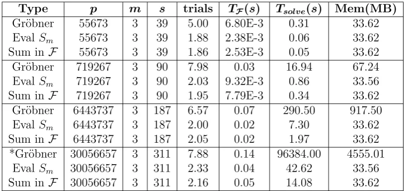
We ran experiments in Magma V2.21-6 [BCP97] with m = 3 and m = 4 to time
• the Algorithm 2.5 first given in [APS18] (called Type Gr¨obner),
• our Algorithm 3.1 (called Type Eval Sm),
• our Algorithm 3.1 using the evaluation for Sm described in Lemma 5.1
(called Type Eval Sm †),
• our Algorithm 4.1 (Type Sum in F),
all with the same parameters. Seemath.ie/ecdlp/ecdlp.htmlfor a Magma implementation of all three algorithms.
We have used a factor base size of s = dp1/me in line with [APS18]. The
results are summarised in Tables 2 and 3, where
• TF(s) denotes the time in seconds it took to compute the factor bases
(step 1 of the algorithms),
• Tsolve(s) denotes the time in seconds it took to find a solution (step 2),
• we did not include the timings for step 3 as they are negligible,
Remark 7.1: The experiments in Table 2 clearly show that for those field sizes our Algorithm 4.1 is the fastest, which agrees with the complexity analysis. Both our algorithms are much faster than Algorithm 2.5 given in [APS18], and that paper shows that their algorithm is in turn faster than the one in [PKM16].
Remark 7.2: As we remarked in section 6, the experiments also show that we need to run several Gr¨obner basis computations in order to solve the discrete logarithm problem using the approach reported in [APS18] (Algo-rithm 2.5).
Remark 7.3: As expected by Remark 6.1 and Remark 6.2, when m = 4, more trials are needed before a relation in the factor base is found, suggesting that the size of the factor base is too small. In fact, the complexity of our Algorithm 3.1 and Algorithm 4.1 grows with m so it may be an advantage to keep to m = 3 and increase the size of the factor base.
Remark 7.4: Table 3 shows that using the evaluation function for Sm
de-scribed in Lemma 5.1 significantly speeds up Algorithm 3.1 for m = 4. It even outperforms Algorithm 4.1 for small values of p.
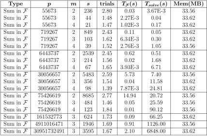
Remark 7.5: Table 4 shows experimental results for s = (m!·p·21−m)1/m using our Algorithm 4.1, over prime fields of bigger size. (This choice of s
gives a probability of obtaining a relation in the factor base of approximately 1 according to Remark 6.1.) The other algorithms could not finish in reason-able time withpthis size. They again show thatm= 3 is faster than m= 4. For m = 2, step 2 of the algorithm (Tsolve(s)) is faster than for m = 3, but
building the factor base (TF(s)) takes more time, so overall m = 2 is slower
than m = 3. So it seems that for Algorithm 4.1,m= 3 is the best choice.
Remark 7.6: Both versions of our algorithm require much less memory than the Gr¨obner basis approach.
Type p m s trials TF(s) Tsolve(s) Mem(MB)
Gr¨obner 55673 3 39 5.00 6.80E-3 0.31 33.62
Eval Sm 55673 3 39 1.88 2.38E-3 0.06 33.62
Sum inF 55673 3 39 1.86 2.53E-3 0.05 33.62
Gr¨obner 719267 3 90 7.98 0.03 16.94 67.24
Eval Sm 719267 3 90 2.03 9.32E-3 0.86 33.56
Sum inF 719267 3 90 1.95 7.79E-3 0.34 33.62
Gr¨obner 6443737 3 187 6.57 0.07 290.50 917.50
Eval Sm 6443737 3 187 2.00 0.02 7.30 33.62
Sum inF 6443737 3 187 2.05 0.02 1.97 33.62
*Gr¨obner 30056657 3 311 7.88 0.14 96384.00 4555.01
Eval Sm 30056657 3 311 2.33 0.04 42.62 33.56
Sum inF 30056657 3 311 2.16 0.05 14.08 33.62
Table 2: Average values on 100 experiments for eachp(the one marked with * was only run 8 times). Type Gr¨obner denotes Algorithm 2.5, Eval Sm
denotes Algorithm 3.1, Sum in F denotes Algorithm 4.1
Type p m s trials TF(s) Tsolve(s) Mem(MB)
Gr¨obner 55673 4 16 33.89 0.02 0.50 33.62
Eval Sm 55673 4 16 3.35 2.84E-3 0.79 33.62
Eval Sm † 55673 4 16 3.14 2.02E-3 0.18 33.62
Sum in F 55673 4 16 2.76 1.93E-3 0.20 33.62
Gr¨obner 719267 4 30 35.47 0.06 19.19 33.62
Eval Sm 719267 4 30 3.42 4.86E-3 9.50 33.62
Eval Sm † 719267 4 30 2.89 3.72E-3 1.22 33.62
Sum in F 719267 4 30 3.23 3.67E-3 1.54 33.56
Gr¨obner 6443737 4 51 32.92 0.09 412.00 169.34
Eval Sm 6443737 4 51 3.17 8.19E-3 66.25 33.62
Eval Sm † 6443737 4 51 3.72 8.70E-3 11.08 33.62
Sum in F 6443737 4 51 3.69 9.00E-3 9.03 33.62
Eval Sm 30056657 4 75 3.06 0.01 288.50 33.56
Eval Sm † 30056657 4 75 3.08 0.01 38.75 33.62
Sum in F 30056657 4 75 3.42 0.02 37.00 33.62
Table 3: Average values on 100 experiments for each p. Type Gr¨obner de-notes Algorithm 2.5, Eval Sm denotes Algorithm 3.1, Eval Sm † denotes
Type p m s trials TF(s) Tsolve(s) Mem(MB)
Sum inF 55673 2 236 2.80 0.03 3.67E-3 33.56
Sum inF 55673 3 44 1.48 2.27E-3 0.04 33.62
Sum inF 55673 4 21 1.47 1.02E-3 0.17 33.62
Sum inF 719267 2 849 2.43 0.11 0.05 33.62
Sum inF 719267 3 103 1.62 6.34E-3 0.30 33.62
Sum inF 719267 4 39 1.52 2.76E-3 1.05 33.56
Sum inF 6443737 2 2539 2.45 0.62 0.51 33.62
Sum inF 6443737 3 214 1.56 0.02 1.68 33.62
Sum inF 6443737 4 67 1.65 3.93E-3 6.71 33.62
Sum inF 30056657 2 5483 2.59 5.73 7.40 33.56
Sum inF 30056657 3 356 1.54 0.04 11.58 33.62
Sum inF 30056657 4 98 1.39 7.87E-3 24.81 33.62
Sum inF 75426619 2 8685 2.77 14.94 20.72 33.56
Sum inF 75426619 3 484 1.46 0.05 25.59 33.56
Sum inF 75426619 4 123 1.84 0.01 90.12 33.56
Sum inF 161532773 3 624 1.73 0.09 66.25 33.62
Sum inF 4911016471 3 1946 1.69 0.91 1126.00 33.56
Sum inF 30951732491 3 3595 1.67 2.10 6848.00 33.62
Table 4: Average values on 100 experiments for eachp using Algorithm 4.1
References
[APS18] Alessandro Amadori, Federico Pintore, and Massimiliano Sala. On the discrete logarithm problem for prime-field elliptic curves. Finite Fields and Their Applications, 51:168 – 182, 2018.
[BCP97] Wieb Bosma, John Cannon, and Catherine Playoust. The Magma algebra system. I. The user language. J. Symbolic Comput., 24(3-4):235–265, 1997. Computational algebra and number theory (London, 1993).
[CG17] Alessio Caminata and Elisa Gorla. Solving multivariate poly-nomial systems and an invariant from commutative algebra. 06 2017. https://eprint.iacr.org/2017/593.
[FHJ+14] Jean-Charles Faug`ere, Louise Huot, Antoine Joux, Gu´ena¨el Re-nault, and Vanessa Vitse. Symmetrized summation polynomials: Using small order torsion points to speed up elliptic curve index calculus. Advances in Cryptology – EUROCRYPT 2014 Lecture Notes in Computer Science, 8441:40–57, 2014.
[Gau09] Pierrick Gaudry. Index calculus for abelian varieties of small di-mension and the elliptic curve discrete logarithm problem. Jour-nal of Symbolic Computation, 44(12):1690–1702, 2009.
[JV11] Antoine Joux and Vanessa Vitse. A variant of the f4 algorithm. In Aggelos Kiayias, editor,Topics in Cryptology – CT-RSA 2011, pages 356–375, Berlin, Heidelberg, 2011. Springer Berlin Heidel-berg.
[JV13] Antoine Joux and Vanessa Vitse. Elliptic curve discrete logarithm problem over small degree extension fields.J. Cryptol., 26(1):119– 143, 2013.
[KV05] Erich Kaltofen and Gilles Villard. On the complexity of comput-ing determinants.Computational Complexity, 13(3-4):91–130, feb 2005.
[Laz83] D. Lazard. Gr¨obner bases, gaussian elimination and resolution of systems of algebraic equations. In J. A. van Hulzen, editor, Com-puter Algebra, pages 146–156, Berlin, Heidelberg, 1983. Springer Berlin Heidelberg.
[MP15] Michael Monagan and Roman Pearce. A compact parallel imple-mentation of f4. In Proceedings of the 2015 International Work-shop on Parallel Symbolic Computation, PASCO ’15, pages 95– 100, New York, NY, USA, 2015. ACM.
[MvOV96] A. Menezes, P. van Oorschot, and S. Vanstone. Handbook of Applied Cryptography. CRC Press, 1996.
[PKM16] Christophe Petit, Michiel Kosters, and Ange Messeng. Algebraic approaches for the elliptic curve discrete logarithm problem over prime fields. Public-Key Cryptography, 9615:3–18, 2016.
[Sem04] Igor Semaev. Summation polynomials and the discrete logarithm problem on elliptic curves. Cryptology ePrint Archive, Report 2004/031, 2004. http://eprint.iacr.org/2004/031.