Computing Optimal Ate Pairings on Elliptic Curves with Embedding Degree $9,15$ and $27$

(will be inserted by the editor)

Computing Optimal Ate Pairings on Elliptic Curves

with Embedding Degree

9

,

15

and

27

Emmanuel Fouotsa · Nadia El Mrabet · Aminatou Pecha

10 November 2018

Abstract Much attention has been given to efficient computation of pairings on elliptic curves with even embedding degree since the advent of pairing-based cryptography. The existing few works in the case of odd embedding degrees require some improvements. This paper considers the computation of optimal ate pairings on elliptic curves of embedding degrees k = 9,15 and 27 which have twists of order three. Mainly, we provide a detailed arithmetic and cost estimation of operations in the tower extensions field of the corresponding extension fields. A good selection of parameters enables us to improve the theoretical cost for the Miller step and the final exponentiation using the lattice-based method comparatively to the previous few works that exist in these cases. In particular fork= 15 andk= 27 we obtained an improvement, in terms of operations in the base field, of up to 25% and 29% respectively in the computation of the final exponentiation. Also, we obtained that elliptic curves with embedding degreek= 15 present faster results than BN12 curves at the 128-bit security levels. We provided a MAGMA implementation in each case to ensure the correctness of the formulas used in this work.

Keywords Elliptic Curves·Optimal Pairings·Miller’s algorithm·Extension fields arithmetic·Final exponentiation

E.Fouotsa

Department of Mathematics, Higher Teacher Training College, University of Bamenda

E-mail: emmanuelfouotsa@yahoo.fr

N. El Mrabet

LIASD, Universit´e Paris 8, 93526 Saint Denis Cedex (France)

SAS-CMP Gardanne, France

A. Pecha

LIASD,Universit´e Paris 8, 93526 Saint Denis Cedex (France)

Mathematics Subject Classification (2000) 14H52·1990S

1 Introduction

Pairings are bilinear maps defined on the group of rational points of elliptic or hyper elliptic curves [40]. They enable to realise many cryptographic proto-cols such as the Identity-Based Cryptosystem [10], Identity-Based Encryption [12], the Identity-Based Undeniable Signature [30], Short Signatures [11] or Broadcast Encryption [19]. A survey of some applications of pairings can be found in [16], [9, Chapter X]. These many applications justify the research on the efficient computation of pairings. Generally, let E be an ordinary el-liptic curve defined over a finite field _Fp and r a large prime divisor of the

order of the groupE(_Fp). The embedding degree ofE with respect tor and

the prime number p is the smallest integer k such that r | pk _{−1. The ρ}

-value of the elliptic curve E is the value logp/logr measuring the size of the base field relatively to the size r of a subgroup of E(Fp). The Tate pairing

and its variants are the most used in cryptography. They map two linearly independent points of the subgroup of order r of E(Fpk) to the group of r

-th roots of unity in -the finite fieldFpk. The computation of the Tate pairing

and its variants consists of an application of the Miller algorithm [35] and a final exponentiation. Efficient computation of pairings requires construction of pairing-friendly elliptic curves over Fp with prescribed embedding degree

k (see for example [8] or [17]) and efficient arithmetic in the towering fields associated to _Fpk (see [27], [20], [25], [14]). A lot of work has been done for

shortening the Miller loop leading to the concept of pairing lattices [22], or the optimal pairing described by Vercauteren which can be computed with the smallest number of iterations in the Miller algorithm [39]. Due to these advances, the final exponentiation step has became a serious task. In this work, we concentrate on elliptic curvesEover_Fpwith embedding degree 9,15

and 27. These curves admit twists of degree three which enable computations

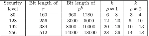
Security Bit length of Bit length of k k

level r pk _ρ

≈1 ρ≈2

80 160 960−1280 6−8 3−4

128 256 3000−5000 12−20 6−10

192 384 8000−10000 20−26 10−13

256 512 14000−18000 28−36 14−18

Table 1 Bit sizes of curves parameters and corresponding embedding degrees to obtain commonly desired levels of security.

Indeed according to the first analysis of this article, as for instance in [21],[4] the security level for elliptic curves with friable embedding degree should be taken greater than those presented in Table 1. The main consequence is that elliptic curves with embedding degree 12 or 18 may not be the one assuring a nice ratio between the security level and the arithmetic. Elliptic curves with odd embedding degree could become interesting and more efficient than el-liptic curves with even embedding degree. Also it is also noticed that elel-liptic curves with odd embedding degree especially with k = 27 may be suitable for computing product of pairings [41]. In this work we consider the following parameter’s sizes (p≈2343_{, r ≈2}257_{, ρ = 1.33), (p≈2}575_{, r ≈2}385_{, ρ= 1.5),} (p≈2579_{, r ≈2}514_{, ρ = 1.12) for curves with k= 9,15,27 respectively. This} corresponds to the 128,192 and 256-bit security levels respectively according to recommendations in Table 1 [17]. However, considering the recent recom-mendations based on the advances on Discrete Logarithm computation with the Number Field Sieve (NFS) algorithm and its variants ([26], [5], [34], [4]) the security level provided by the above parameters may reduce. Indeed, let 2−dexp((c+o(1))(logQ)1/3( log logQ)2/3 wheredandc are constants, be the runing time of the NFS algorithm, with Q=pk. The base-two logarithm of this runtime with (o(1) = 0) givesS(Q, c, d) =c(lge)(logQ)1/3(loglogQ)2/3−d. We then know that the constants c and d, the embedding degree k and the security level l must satisfy the following Pollard-Rho security and variants of NFS security constraints logQ/k ≥ 2ρl and S(Q, c, d) ≥ l. Therefore the previous parameters provide a security level of 109,168,214 bits instead of 128,192,256-bit respectively for curves with k = 9,15,27. But for now we still consider in Section 4, 5 and 6 recommendation from Table 1 in order to make a fair comparison with previous works. Later in section 8, we consider advances in discrete logarithm computation and provide tentative updated pa-rameters at the 128,192,256 bits respectively for curves withk= 9,15,27. So we proposed a detailed arithmetic in the towering fields associated to the fields Fp9,_Fp15 and_Fp27. The lattice-based method explained by Fuentes et al.[18]

is applied to compute the final exponentiation in the casesk= 9,15. We also find a simple expression and explicit cost evaluation for the optimal pairing in the cases k= 9 andk= 15 comparatively to the work in [36]. The results obtained are an improvement with respect to previous works [29], [36] and [41] respectively fork= 9,15 and 27. Precisely, our contributions (see Table 3 and subsection 8.4 for comparison) in this work are:

1. Determination of an explicit cost of the computation of the optimal pairing for elliptic curves stated above. This includes a good selection of parameters for a shorter Miller loop and an efficient exponentiation. In particular, we saved one inversion in _Fp27 for the computation of the Miller loop in the

casek= 27.

2. Details on the arithmetic in the tower of subfields of _Fp9,_Fp15 and _Fp27.

Especially, we give the cost of the computation of Frobenius maps and In-versions in the cyclotomic subgroups of_F∗_p9,F∗_p15 andF∗_p27, (see Appendices

3. Improvement of the costs of the final exponentiation by saving 828M1+ 145S1,1170M1 + 7767S1 and 8676M1 + 32136S1 operations for elliptic curves of embedding degrees 9,15 and 27 respectively, comparatively to previous works in these cases; where Mk, Sk represent the costs of

multi-plication and squaring in the finite field_Fpk.

4. In Section 8 we look for new parameters considering the advances in Dis-crete Logarithm computation to update the cost of the optimal ate pairings on the studied curves at the 128,192 and 256-bit security levels. We then compare our results with known curves such as BN and BLS curves. In particular we obtained that elliptic curves with embedding degree k= 15 present faster results than BN12 curves at the 128-bit security levels. We also provide a MAGMA implementation in each case to ensure the cor-rectness of the formulas used in this work. The code is available in [?].

The rest of this paper is organised as follows: In Section 2 we briefly present the Tate and ate pairings together with the Miller algorithm for their efficient computation, we also recall the concept of optimal ate pairing and the lattice-based method for computing the final exponentiation. Sections 4, 5 and 6 present arithmetic in subfields, and costs estimation of the Miller step and the final exponentiation when considering the embedding degrees k = 9,15 and 27 respectively. Each of these sections includes a comparative analysis with previous work. Section 7 presents a general comparison of the results obtained in this work and the previous results in the literature. In Section 8 we look for new parameters considering the advances in Discrete Logarithm computation to update the cost of the optimal ate pairings on the studied curves at the 128,192 and 256-bit security levels. We then compare our results with known curves such as BN and BLS curves. We conclude the work in Section 9 in which we suggest as future work the search for parameters to have subgroup secure ordinary curves [6] and to ensure protection againstsmall-subgroup attacks[32].

Notations

The following notations are used in this work.

Mk,Sk,Ik : Cost of multiplication, squaring and inversion in the fieldFpk, for

any integerk.

2 Background and previous works

2.1 Pairings and the Miller Algorithm

LetEbe an elliptic curve defined overFp, a finite field of characteristicp >3.

Let r be a large prime factor of the group order of the elliptic curve. Let

m ∈ Z and P ∈ E(Fp)[r] a point of E of order r with coordinates in Fp.

Letfm,P a function with divisor Div (fm,P) =m(P)−([m]P)−(m−1)(O)

the embedding degree of E with respect to r. We also consider the point

Q ∈ E(Fpk)[r] of E of order r with coordinates in _Fpk and denote µr the

group ofr-th roots of unity inF∗pk. The reduced Tate pairinger is a bilinear

and non degenerate map defined as

er:E(Fp)[r]×E(Fpk)[r]→µr,(P, Q)7→fr,P(Q)

pk−1

r

To define a variant of the Tate pairing called ate pairing [23], let’s denote [i] :P 7−→[i]P the endomorphism defined on E(_Fp) which consists to addP

to itselfi times. Letπp:E Fp→E Fp,(x, y)7→(xp, yp) be the Frobenius

endomorphism on the curve where _Fp is the algebraic closure of the finite

field_Fp. The relation between the tracetof the Frobenius endomorphism and

the group order is given by [40, Theorem 4.3]:]E(Fp) =p+ 1−t andπp has

exactly two eigenvalues 1 andp. This enables to considerP ∈G1=E Fp[r]∩

Ker(πp−[1]) = E(Fp)[r] and Q ∈ G2 = E Fp[r]∩ Ker(πp−[p]). The ate

pairing is defined as follows:

eA:G2×G1→µr; (Q, P)7→ft−1,Q(P)

pk−1

r .

In all variants of pairings, one needs a value fm,U(V) which is efficiently

computed thanks to the Miller algorithm [35]. Indeed denotehR,S a rational

function with divisor Div(hR,S) = (R) + (S)−(S+R)−(O) where R and

S are two arbitrary points on the elliptic curve. In the case of elliptic curves in Weierstrass form, hR,S =

`R,S

vR+S where `R,S is the straight line containing R andS andvR+S is the corresponding vertical line passing throughR+S.

Miller uses the double-and-add method as the addition chains for m (see [3, Chapter 9] for more details on addition chains) to compute f := fm,U(V).

Writem=mn2n+...+m12 +m0 >0 with mi ∈ {−1,0,1}, the (modified)

Miller algorithm that efficiently computes the pairingfm,U(V)(p

k_−1)/r

of two pointsU andV is given as follows:

1: Setf ←1 andR←U

2: Fori=n−1down to0do

3: f ←f2_·h

R,R(V), R←2R Doubling step

5: if mi= 1then

6: f ←f·hR,U(V) R←R+U,end if Addition step

7: if mi=−1 then

8: f ←f /hR,U(V) R←R−U, end for Addition step

10: returne=fpkr−1 Final exponentiation

2.2 Use of Twists

Twists of elliptic curves enable to efficiently compute pairings. Indeed, in the Miller algorithm the doubling of a point (line 3) and the addition of points (lines 6 and 8) are done in the extension field _Fpk in the case of the ate

pairing. The use of twists enables to perform these operations rather in a sub-field of _Fpk and also leads to the denominator elimination. More precisely, a

twist of an elliptic curve E defined over a finite field _Fp is an elliptic curve

E0 defined over _Fp which is isomorphic to E over an algebraic closure of Fp. The smallest integer d such that E and E0 are isomorphic over Fpd is

called the degree or the order of the twist. Elliptic curves of embedding degree

k = 9,15 and k = 27 admit twists of order three. Explicit constructions of such curves can be found in [33], [15] and [7]. The general equation of these curves is given by E : y2 =x3+b. The equation defining the twist E0 has the formy2=x3+bω6 where{1, ω, ω2}is the basis of theFpk/3-vector space Fpk and the isomorphism between E0 and E is ψ : E0 −→ E; (x0, y0) 7−→

(x0/ω2, y0/ω3). Using this isomorphism, points Qin G2 can be instead taken as (xω−2_{, yω}−3_{) where (x, y) ∈ E}0₍

Fpk/3). The function hR,S is defined by

hR,S(x, y) =

y+λ(xR−x)−yR

x−xR+S where λ is the slope of the line passing through R and S. Observe that using the equation of the curvey2 _{= x}3_{+b one has}

x−xR+S =

y2−y2_R+S x2_+x

R+Sx+x2R+S

. In the present case of ate pairing, the addition

R+Sis performed in the extension fieldFpkand the functionhR,Sis evaluated

at a point (xP, yP)∈E(Fp). So using the twist, the pointsR,SandR+Sare

taken in the form (xω−2, yω−3) where (x, y)∈ E0(Fpk/3). Therefore we have

hR,S(xP, yP) =

(yPω5+λ(xRω2−xPω4)−yRω2)(x2Pω4+xR+SxPω2+x2R+P)

y2

Pω9−y2R+Pω3

. We observe that the denominator is an element of the subfield _Fpk/3 and so will be sent

to 1 during the final exponentiation (line 10 in the Miller algorithm) since

pk/3_{−1 is a factor ofp}k_{−1. Consequently we simply ignore that denominator}

in the Miller algorithm for an efficient computation. More details on twists can be found in [13].

2.3 Optimal Pairings

The reduction of Miller’s loop length is an important way to improve the com-putation of pairings. The latest work is a generalized method to find the short-est loop, which leads to the concept of optimal pairings due to Vercauteren [39]. Letλ=mrbe a multiple ofrsuch thatr_-mand writeλ=Pl

i=0cipi=h(p),

(h(z) ∈_Z[z]). Recall that hR,S is the Miller function defined in section 2.1.

Fori= 0,· · ·l setsi=P l

j=icjpj; then the map

eo:G2×G1 → µr

(Q, P) 7−→Ql i=0f

pi

ci,Q(P)·

Ql−1

i=0h[si+1]Q,[cipi]Q(P)

defines a bilinear pairing and non degenerate if

mkpk6= ((pk−1)/r)·Pl

i=0icipi−1 modr.

The coefficients ci : i = 0,· · · , l can be obtained from the short vectors

ob-tained from the lattice

L=



    

r 0 0 · · · 0

−p 1 0 · · · 0

−p2 _{0 1 · · · 0}

· · · · −pφ(k)−1 _{0 0 · · · 1}



    

(2)

2.4 Final Exponentiation and the Lattice-Based Method for its Computation

The result of the Miller loop’s step is raised to the power pk_r−1. This step is called the final exponentiation (line 10 in Miller’s algorithm). The efficient computation of the final exponentiation has became a serious task. Observe that this exponent can be divided into two parts as follows:

pk₋₁

r =

_pk₋₁

φk(p)

·

_φ k(p)

r

where φk(x) is the k-th cyclotomic polynomial. The final exponentiation is

therefore computed as fpkr−1 =

fpk

−1

φk(p) φkr(p)

. The computation of the first

part A=fpk

−1

φk(p) _{is generally inexpensive as it consists of few multiplications,}

inversion andp-th powering inFpk. The second partA φk(p)

r is considered more

difficult and is called the hard part. An efficient method to compute the hard part is described by Scottet al.[37]. They suggested to writed=φk(p)

r in base

pasd=d0+d1p+...+dφ(k)−1pφ(k)−1and find a short vectorial addition chains to compute Ad _{much more efficiently than the naive method. In [18], based}

on the fact that a fixed power of a pairing is still a pairing, Fuentes et al.[18] suggested to apply Scottet al.’s method with a power of any multipled0 ofd

withrnot dividingd0. This could lead to a more efficient exponentiation than computingAd _{directly. Their idea of finding the polynomial d}0_{(x) is to apply}

theLLL-algorithm to the matrix formed by_Q-linear combinations of the el-ements d(x), xd(x), ..., xdegr−1_{d(x). They successfully applied the method in} the case of elliptic curves of embedding degrees 8,12 and 18 [18]. In Sections 4 and 5 we apply this method to improve the computation of the final exponen-tiation for elliptic curves of embedding degreek= 9 and 15. A clever method was used by Zhanget al. [41] to compute the final exponentiation in the case

3 Arithmetic in the tower of subfields ofFp9,_Fp27 and _Fp15

A pairing is computed as an element of the extension field _Fpk. But its

ef-ficient computation depends on the arithmetic of subfields of _Fpk which is

generally organised as tower of subfields extensions. In this section we recall the tower extension of finite fields _Fp9,_Fp27 and _Fp15. We also give explicit

cost of the arithmetic operations. For extension-field arithmetic in _Fp9 and Fp27 we consider p≡1 mod 3 motivated by the work of Barreto et al.[7] on

the construction of elliptic curves of embedding degree 9 and 27. This implies thatFpk can be represented as_Fpk/3[X]/(X3−α), fork= 3i, i= 1,2,3 where

αis a cubic non residue modulo p. Sincep≡1 mod 3 we have that X3₋₇ irreducible overFp. Therefore cubic extensions will be constructed using the

polynomialsX3−αi where αi = 71/3

i−1

. A tower extension forFp27 together

with the one for_Fp9 are then given by:

Fp3=_Fp[u] with u3= 7 Fp9 =_Fp3[v] with v3= 71/3 Fp27 =_Fp9[w] with w3= 71/9

The costs of the computation of the Frobenius maps and cyclotomic inversions are given in Lemma 1 for the extensionFp9. The proof of this Lemma is given

in Appendix A.

Lemma 1 In the finite fieldFp9,

1. The computation of the p3;p6-Frobenius maps costs6M1

2. The computation of the p;p2;p4;p5;p7;p8-Frobenius maps costs 8M1 3. The inverse of an element α of the Gφ3(p3)-order cyclotomic subgroup is

computed as α−1_=αp3_·αp6 _{and the cost is36S} 1

Similarly, in the finite field _Fp27 the Lemma 2 gives the costs of the

com-putation of the Frobenius maps and cyclotomic inversions. The proof of this Lemma is given in Appendix B.

Lemma 2 In the finite fieldFp27,

1. The computation of the p3;p6;p9-Frobenius maps costs 18M1

2. The computation of the p;p2;p4;p5;p7;p8-Frobenius maps costs 26M1 3. The inverse of an element α of the Gφ3(p9)-order cyclotomic subgroup is

computed as α−1_=αp9_·αp18 _{and the cost is216S} 1

In the case of Fp15, we consider pairing friendly curves over _Fp where

p ≡ 1 mod 5 [15]. According to [31, Theorem 3.75] the polynomial X5_−α is irreducible overFp[X] if and only ifαis neither a cubic root nor a fifth root

inFp. A tower extension forFp15 can be constructed as follows:

Fp5=_Fp[u] with u5= 7

Fields Operations Costs

Fp3

MultiplicationM3 6M1

SquaringS3 5S1

InversionI3 I1+ 9M1+ 2S1

Fp9

MultiplicationM9 36M1

SquaringS9 25S1

InversionI9 I1+ 63M1+ 12S1

Frobeniusp3_;p6 _6M

1

Frobeniusp;p2_;p4_;p5_;p7_;p8 _8M 1

Inversion inG_φ

3(p3) 18M1+ 15S1

Fp27

MultiplicationM27 216M1

SquaringS27 125S1

InversionI27 I1+ 387M1+ 62S1

Frobeniusp3_;p6_;p9 _18M 1

Frobeniusp;p2_;p4_;p5_;p7_;p8 _26M 1

Inversion inGφ3(p9) 108M1+ 75S1

Fp5

MultiplicationM5 9M1

SquaringS5 9S1

InversionI5 1I1+ 45M1+ 5S1

Fp15

MultiplicationM15 45M1

SquaringS15 45S1

InversionI15 1I1+ 126M1+

23S1

Frobeniusp5_;p10 _10M

1

Frobeniusp;p2_;p3_;p4_;p6_;p7_;p8_;p9 _14M 1

Inversion inG_φ3(p5₎ 27M1+ 27S1

Table 2 Cost of operations in extension fields from [29], [36] and [41] and this work (see Appendix A, B and C)

Our main contribution in this section is the computation of Frobenius maps and the inversions in theφn(.)-order cyclotomic subgroup ofF∗pk. The costs of

the computation of the Frobenius maps and cyclotomic inversions are given in Lemma 3.

Lemma 3 In the finite fieldFp15,

1. The computation of the p5_;p10_{-Frobenius maps costs10M} 1

2. The computation of thep;p2_;p3_;p4_;p6_;p7_;p8_;p9_{-Frobenius maps costs14M} 1 3. The inverse of an element α of the Gφ3(p5₎-order cyclotomic subgroup is

computed as α−1=αp5·αp10 and the cost is54S1

Proof The proof is given in Appendix C.

4 Elliptic Curves with Embedding Degree 9

This section describes the computation of the optimal ate pairing (Miller step and the final exponentiation) on the parameterized elliptic curve defined in [33]. The correctness of the results can be verified with the MAGMA code available in [?]. This family of elliptic curves has embedding degree 9 and a

ρ-value 1.33 and is parameterized by :

p= ((x+ 1)2+ ((x−1)2(2x3+ 1)2)/3)/4

r= (x6_+x3_{+ 1)/3}

t =x+ 1

(3)

4.1 Optimal ate pairing

Based on the general framework described by Vercauteren in [39], the short vector obtained from the latticeL defined by equation (2) gives the optimal function h(z) = P5

i=0cizi =x−z ∈ Z[z]. A straightforward application of formula (1) yields the optimal pairing

eo:G2×G1−→µr

(Q, P) 7−→fx,Q(P)

p9−1

r

4.2 Cost of the execution of the Miller loop

The Miller loop consists of the doubling steps (line 3 in the Miller algorithm) and addition steps (line 6 or 8 in the Miller algorithm). These steps use the Miller functionhR,S either in affine coordinates or in projective coordinates.

The work of Zhanget al.[41, Section 3] presents the currently fastest formulas in projective coordinates. The doubling step costs 9M1+ 3M3+ 9S3 and the cost of the addition step is 9M1+ 12M3+ 5S3. For an explicit cost of the computation of fx,Q(P), we wrote a Pari/GP code to find a suitable xwith

low Hamming weight and minimal number of bits for the 128 bit-security level according to Table 1. The best value we were able to find isx= 243₊₂37₊₂7₊₁ which gives anr(x) prime of 257 bits andp(x) a prime of 343 bits. The values

pand xare both congruent to 1 modulo 6 so that the corresponding elliptic curve is y2 _{= x}3_{+ 1 [29]. The computation of f}

x,Q(P) therefore costs 43

doubling steps, 3 additions, 42 squaring and 45 multiplications in_Fp9. Thus

4.3 Cost of the computation of the final exponentiation

As explained in Section 2, the final exponentiation in this case can be divided as

f(p9−1)/r=fp3−1

(p6_+p3_+1)/r

=fp3−1

d

. We then used the lattice method described by Fuentes et al.[18] that we briefly explained in Section 2.4. It is applied to the following matrix in which the coefficient 243 is used to obtain integer entries asd= (p6_+p3_{+ 1)/ris a polynomial with rational coefficients}

M =



      

243d(x) 243xd(x) 243x2_d(x) 243x3_d(x) 243x4_d(x) 243x5_d(x)



      

(4)

We obtain the following multiple of d: d0 =x3d=k0+k1p+k2p2+k3p3+

k4p4+k5p5 where the polynomialski, i= 0, ...,5 are as follows

k0=−x4+ 2x3−x2, k1=−x3+ 2x2−x, k2=−x2+ 2x−1,

k3=x7−2x6+x5+ 3, k4=x6−2x5+x4, k5=x5−2x4+x3 They verify the relations (see the code in [?] for verification)

k2=−(x−1)2, k1=xk2, k0=xk1, k5=−xk0, k4=xk5, k3=xk4+3 If we setA=fp3₋₁

then

– The cost for the computation of A is 1 p3_{-Frobenius, 1 Inversion in} Fp9

and 1 multiplication in_Fp9.

– The cost of the computation ofAk0_{, A}k1 _andAk4 _{is 3 exponentiations by}

x,

– The cost of the computation of Ak5 _{is one inversion in the cylotomic}

sub-group and one exponentiation by x.

– The cost of the computation of Ak2 _{is one inversion in the cyclotomic}

subgroup and two exponentiations by (x−1).

– The cost of the computation of Ak3 _{is 2 multiplications, one squaring and}

one exponentiation byx.

Note that the inversion in the cyclotomic subgroupGφ3(p3)of orderp

6_+p3_{+ 1} is computed asA−1 _=Ap3 _·Ap6 _{(see Appendix A for details and cost). The}

cost for the hard partAd0 _{is then 2 exponentiations byx−1, 5 exponentiations}

byx, 7 multiplications in Fp9, one squaring in_Fp9, two cyclotomic inversions

IG_φ

3 (p3 ) andp, p

2_{, p}3_{, p}4_{, p}5_{-Frobenius maps. Using the value ofxgiven above,} one exponentiation byxcosts 43S9+3M9whereas one exponentiation byx−1 costs 43S9+2M9. Finally the hard part costs 2(43S9+2M9)+5(43S9+3M9)+ 7M9+1S9+2IG_φ

3 (p3 ) = 302S9+26M9+2IGφ3 (p3 )andp, p

2_{, p}3_{, p}4_{, p}5_-Frobenius maps. The total cost of the final exponentiation is 1I9+27M9+302S9+2IG_φ

3 (p3 )

4.4 Improvement and comparison with previous work

From the results in [29], the hard part costs 309S9+ 50M9andp, p2, p3, p4, p5 -Frobenius maps. If we include the cost 1I9+ 1M9 and p3-Frobenius for the easy part and using the arithmetic in Table 2, the overall cost isI1+ 1115M1+ 7592S1for this work andI1+ 1943M1+ 7737S1for Le etal.[29]. We therefore save 828M1+ 145S1comparatively to their work. Although the sizes of pare 343 bits in this work and 348 bits in [29], the cost of a multiplication is almost the same in the two corresponding fields (see section 8.4).

5 Elliptic Curves with Embedding Degree 15

In this section we give explicit formulas together with their cost for the Miller loop in the computation of the optimal ate pairing. We then compute the cost of the final exponentiation on the parameterized elliptic curve defined in [15]. The correctness of the results can be verified in [?]. This family of elliptic curves has embedding degree 15 and aρ-value 1.5 and is parameterized by :

p= (x12_−2x11_+x10_+x7_−2x6_+x5_+x2_{+x+ 1)/3}

r=x8−x7+x5−x4+x3−x+ 1

t =x+ 1

(5)

5.1 Optimal ate pairing

The Vercauteren approach described in [39] enabled us to obtain the short vector from the lattice L defined by equation (2) which lead to the optimal function h(z) = P5

i=0cizi =x−z ∈ Z[z]. A straightforward application of formula (1) yields the optimal pairing

eo:G2×G1−→µr

(Q, P) 7−→fx,Q(P)

p15−1

r

5.2 Cost of the computation of the Miller loop

In this section, we consider the Miller function given in affine coordinates, following the analysis of Lauter et al. [28] who suggested to use affine coor-dinates at higher security level. Miller function used for the computation of

fx,Q(P) in this case is described in [41, Table 2] with the fastest cost to date.

At 192 bits security level on elliptic curves withk = 15, the best value of x

loop consists here of computingfx,Qwhich costs 48 doubling steps, 4 additions

steps, 47 squaring and 51 multiplications in Fp15. Considering the currently

fastest cost for doubling and addition step in [41, Table 2], the Miller loop costs 48(15M1+ 3M5+ 2S5+I5) + 4(15M1+ 3M5+ 2S5+I5) + 47S15+ 51M15, which is 51M15+ 156M5+ 780M1+ 47S15+ 104S5+ 52I5. Using the arithmetic in Table 2, the overall cost is 52I1+ 6819M1+ 3311S1. To our knowledge no explicit cost is reported in the literature in the case k = 15 with a specific value ofx.

5.3 Cost of the computation of the final exponentiation

The final exponentiation in this case is written in a different way asf(p15−1)/r₌

fp5₋₁(p10+p5+1)/r

=fp5₋₁d

. This decomposition is used instead of p15_r−1 =

h_p15₋₁ φ15(p) i

·hφ15_r(p)ias usually done, for efficiency reasons in the computation. Ob-serve that p_φ15−1

15(p) =p

7_+p6_+p5_−p2_{−p−1 andφ}

15(p) =p8−p7+p5−p4+p3−p+1 will lead to several multiplications and Frobenius maps operations. Thus the lattice method described by Fuenteset al.[18] that we briefly explained in Sec-tion 2.4 is applied to the following matrixM. In the matrixM the coefficient

59049

19683 is used to obtain integer entries asd= (p

10_+p5_{+ 1)/ris a polynomial} with rational coefficients.

M =         59049 19683d(x) 59049 19683xd(x) 59049 19683x

2_d(x)

. .

59049 19683x

7_d(x)

        (6)

We then obtained the following multiple ofd:d0 = 3x3_d=k

0+k1p+...k9p9 where the polynomialski, i= 0, ...,9 are defined as follows

k0=−x6+x5+x3−x2, k1=−x5+x4+x2−x

k2=−x4+x3+x−1

k3=x11−2x10+x9+x6−2x5+x4−x3+x2+x+ 2

k5=x11−x10−x8+x7+ 3

k4=x11−x10−x9+x8+x6−x5−x4+x3−x2+ 2x+ 2

k6=x10−x9−x7+x6 k7=x9−x8−x6+x5

k8=x8−x7−x5+x4 k9=x7−x6−x4+x3

The polynomials ki : i = 0, ...9 verify the relations (see the code in [?] for

verification)

k2=−(x−1)2(x2+x+ 1), k1=xk2, k0=xk1

k9=−xk0, k8=xk9, k7=xk8

k6=xk7, k5=xk6+ 3, k4=M −(k1+k7)

SetA=fp5−1 then

– The cost for the computation of A is 1 p5-Frobenius,1 Inversion in Fp15

and 1 multiplication inFp15 and .

– The computation of Ak2 _{is 2 exponentiations by x, 2 exponentiations by}

x−1, 2 multiplications and 1 cyclotomic inversion,

– The cost of the computation of the Ak0_,Ak1_,Ak6_,Ak7 _{is 5 exponentiations}

byx, the computation ofAk9 _{costs 1 exponentiation byxand 1 cyclotomic}

inversion,

– The computation ofAk5 _{is 1 exponentiation byx, 2 multiplications and 1}

squaring in_Fp15,

– The computation of Ak4 _{costs 4 multiplications in}

Fp15 and 1 cyclotomic

inversion,

– The computation of Ak3 _{costs 3 multiplications in}

Fp15 and 1 cyclotomic

inversion.

Therefore, the cost of the computation ofAd0 _{is 2 exponentiations byx−1, 9}

exponentiations byx, 20 multiplications, one squaring inFp15, four inversions

in the cyclotomic subgroupGφ3(p5₎of orderp10+p5+ 1 (note thatA−1=Ap 5

· Ap10

see Appendix C for details) and p, p2_{, p}3_{, p}4_{, p}5_{, p}6_{, p}7_{, p}8_{, p}9_-Frobenius maps. Using the value ofxgiven above, the cost of the hard part is 2(48S15+ 3M15)+9(48S15+4M15)+20M15+1S15+4IG_φ

3 (p5 ) = 529S15+62M15+4IGφ3 (p5 )

and p, p2, p3, p4, p5, p6, p7, p8, p9-Frobenius maps. The total cost of the final exponentiation in this work is therefore 1I15+ 529S15+ 63M15+ 4IG_φ

3 (p5 ) and p, p2_{, p}3_{, p}4_,2∗p5_{, p}6_{, p}7_{, p}8_{, p}9_{-Frobenius maps.}

Remark 1 The cost given by Le et al. [29] for the hard part is 11 exponen-tiations by x, 22 multiplications, 2 inversions inFp15 and 9 Frobenius maps.

The authors said that the cost of an inversion inFp15 is free with a reference

to a similar computation but on elliptic curves with even embedding degree, unfortunately we do not see how this is possible. Also, they considered an x

of 64 bits and hamming weight 7 and claimed that the cost is 88M15+ 528S15 instead of 11(6M15+ 64S15) = 88M15+ 704S15. Therefore if we count the 2 inversions in _Fp15 (these inverses are in fact in the cyclotomic subgroup

Gφ3(p5)), then their final cost is 88M15+ 704S15+ 2IGφ3 (p5 ) and 11 Frobenius

maps, whereas our cost is 529S15+ 62M15+ 4IG_φ 3 (p5 ).

5.4 Improvement and comparison with previous work

Considering the previous remark, the cost of the final exponentiation in [29] is 1I15+704S15+89M15+2IG_φ

3 (p5 )andp, p

2_{, p}3_{, p}4_,2∗p5_{, p}6_{, p}7_{, p}8_{, p}9_-Frobenius maps. We observe that we have improved the results by saving 26M15+ 175S15−2IG_φ

3 (p5 ). Using the arithmetic in Table 2, the overall cost is I1+

We therefore save 26M15+ 175S15−2IG_φ

3 (p5 ) = 1170M1+ 7767S1

compara-tively to their work. A MAGMA code for the implementation to ensure the correctness of the decomposition of the final exponentiation and the Miller function is available in [?].

6 Elliptic Curves with Embedding Degree 27

The parameterized elliptic curves with embedding degree 27 is defined in [7]. This family has aρ-value 10/9 and is parameterized by the following polyno-mials:

p= 1/3(x−1)2(x18+x9+ 1) +x r= 1/3(x18+x9+ 1)

t =x+ 1

(7)

6.1 The Miller loop and the final exponentiation

The Miller loop and the final exponentiation has been studied in [41]. They found the optimal functionh(z) =P17

i=0cizi=x−z∈Z[z] and the optimal pairing is given by

eo:G2×G1−→µr; (Q, P)7−→fx,Q(P)

p27−1

r

The authors in [41] used the parameterx= 228_{+ 2}27_{+ 2}25_{+ 2}8₋₂3 _{for their} computation at 256-bit security level. The cost of the Miller step that they obtained is therefore 28(3M9+ 2S9+ 1I9+ 9M1) + 4(3M9+ 2S9+ 1I9+ 9M1) + 27(6S9)+30(6M9)+1I27= 276M9+226S9+32I9+288M1+I27operations. The computation of the final exponentiation in [41] requires 1I27+11M27, 17 powers of x, 2 powers of x−1 and p, p2_{, p}3_{, p}4_{, p}5_{, p}6_{, p}7_{, p}8_,2∗p9_{-Frobenius maps.} Therefore the explicit cost of the final exponentiation is 1I27+ 17(4(6M9) + 28(6S9) + 36M1) + 2(5(6M9) + 28(6S9) + 36M1) + 11(6M9) + 228M1= 1I27+ 648M9+ 3192S9+ 912M1.

Then the explicit cost for the computation of the Miller loop and the final exponentiation given in that work is 12627M1+ 8670S1+ 33I1and 24627M1+ 114998S1+ 1I1 respectively (see [41] for details).

Remark 2 The negative coefficient in the value ofxaffects the efficiency since one full inversion in_Fp27 is required in the Miller algorithm (line 8) and also 19

inversions in the cyclotomic subgroup are required when raising to the power ofxduring the final exponentiation.

6.2 Improvement and comparison with previous work

We use the arithmetic (especially the computation of inversion in the cy-clotomic subgroup) and a specific value of x to improve the costs in [41]. Precisely, a careful search with a Pari/GP code enabled us to find the value

x = 229 _{+ 2}19_{+ 2}17_{+ 2}14 _{so that r has a prime factor of 514 bits length} and the primephas a bit length of 579 for 256-bit security level according to Table 1. An adequate elliptic curve has the equation y2 _=x3_{−2. Although} the corresponding base field is a bit larger (579 bits instead of 573 in [41], butm579≈m573see section 8.4 for notations) and we have an extra doubling step, we avoid the full inversion in Fp27 and 17 inversions in the cyclotomic

subgroup Gφ3(p9₎ when raising to power x. We perform 2 inversions in the

cyclotomic subgroup only when raising to powerx−1. The cost of the Miller loop now becomes 29(3M9+ 2S9+ 1I9+ 9M1) + 3(3M9+ 2S9+ 1I9+ 9M1) + 27(6S9) + 30(6M9) = 276M9+ 226S9+ 32I9+ 288M1. Using the arithmetic in Table 2, the overall cost for the Miller loop is 32I1+ 12240M1+ 6034S1for this work where we saved at least one inversion inFp27.

Our cost for the final exponentiation is 1I27+17(3(6M9)+29(6S9))+2(4(6M9)+ 29(6S9)) + 2IGφ3 (p9 ) + 11(6M9) = 1I27+ 420M9+ 3306S9 + 2IGφ3 (p9 ) and

p, p2_{, p}3_{, p}4_{, p}5_{, p}6_{, p}7_{, p}8_,2∗p9_{-Frobenius maps. Using the arithmetic in Table} 2, the overall cost isI1+15951M1+82862S1for this work. The implementation of this pairing is available in [?].

7 General Comparison

In this section, we summarize the different costs obtained in this work and compare our results with previous works.

Curves References Miller loop Final Exponentiation

k= 9 Previous work [29] No specific cost reported I1+ 1943M1+ 7737S1 128-bit This work 3024M1+ 3060S1 I1+ 1115M1+ 7592S1

k= 15 Previous work [36] No specific cost reported I1+ 4263M1+ 31811S1 192-bit This work 52I1+ 6819M1+ 3311S1 I1+ 3093M1+ 24044S1

k= 27 Previous work [41] 33I1+ 12627M1+ 8670S1 I1+ 24627M1+ 114998S1 256-bit This work 32I1+ 12240M1+ 6034S1 I1+ 15951M1+ 82862S1

Table 3 Comparison of the cost of the Miller loop and the final exponentiation.

If we assume that the cost of a squaring is the same as the cost of a multiplication then the cost of the final exponentiation is I1+ 27137M1 and

8 New Parameters for Optimal Ate pairing on Elliptic Curves with embedding degrees 9,15 and 27

In this section we consider new parameters for parameterized curves of em-bedding degrees 9,15 and 27 at the 128,192 and 256-bit security levels. We consider recent advances on the computation of the discrete logarithm thanks to the Number Field Sieve (NFS) algorithm and its variants described in some papers as mentioned in the introduction. Mostly, the paper of Barbulescu and Duquesne [4] presents a detailed approach for computing new parameters for pairings. Based on their analysis, Scott and Guillevic [38] have proposed ten-tative general recommended parameters for classical security level and that we reproduce here in Table 4.

DL Algorithm AES-128 AES-192 AES-256

NFS 3072 7680 15360

exTNFS 3618 9241 18480

SexTNFS 5004 12871 27410

Table 4 Recommended extension fields size (pk) to obtain desired levels of security [38].

Following the Table 4, we searched for new parameters that will ensure resistance to SexTNFS algorithm at the various security levels for curves of embedding degrees 9,15 and 27.

8.1 New parameters and costs for optimal ate pairing at the 128-bit security level fork= 9 and k= 15

– Case ofk= 9. Following the recommendation from Table 4, we found the valuex= 270_{+ 2}59_{+ 2}46_{+ 2}41_{+ 1. This gives a primepof 559 bits and a} primerof 419 bits. We proceed as described in Section 4 to obtain the cost of the Miller loop and the final exponentiation. The Miller loop costs in this case 70(9M1+ 3M3+ 9S3) + 4(9M1+ 12M3+ 5S3) + 69S9+ 73M9. This is equal to 73M9+ 258M3+ 666M1+ 69S9+ 650S3. Using the arithmetic in Table 2, the overall cost is 4842M1+ 4975S1. Using the value ofxgiven above, the hard part of the final exponentiation costs 2(70S9+ 3M9) + 5(70S9+ 4M9) + 7M9+ 1S9+ 2IG_φ

3 (p3 ) = 491S9+ 33M9+ 2IGφ3 (p3 ) and p, p2_{, p}3_{, p}4_{, p}5_{-Frobenius maps. The total cost of the final exponentiation} is 1I9+ 34M9+ 491S9+ 2IG_φ

3 (p3 ) and p, p

2_,2∗p3_{, p}4_{, p}5_{-Frobenius maps} for a total cost ofI1+ 1367M1+ 12317S1.

– Case ofk= 15. Following the recommendation from Table 4, we found the valuex= 231_{+ 2}19_{+ 2}5_{+ 2}2_{. This gives a primepof 371 bits and a prime}

2, the overall cost is 4020M1+3384S1. Using the value ofxgiven above, the hard part of the final exponentiation costs 2(31S15+ 4M15+ 1IG_φ

3 (p5 )) +

9(31S15+ 3M15) + 20M15+ 1S15+ 4IG_φ

3 (p5 ) = 55M15+ 342S15+ 6IGφ3 (p5 )

andp, p2_{, p}3_{, p}4_{, p}5_{, p}6_{, p}7_{, p}8_{, p}9_{-Frobenius maps. The total cost of the final} exponentiation is I15 + 56M15+ 342S15 + 6IG_φ

3 (p5 ) and p, p

2_{, p}3_{, p}4_{,2 ∗}

p5_{, p}6_{, p}7_{, p}8_{, p}9_{-Frobenius maps for a total cost ofI}

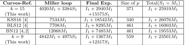
1+ 2940M1+ 15575S1. The following table 5 compares our results with previous results at the 128-bit security level.

Curves-Ref. Miller loop Final Exp. Size ofp Total(S1=M1)

k= 15 4020M1+ 3384S1 I1+ 2940M1 371 I1+ 25919M1

(This work) +15575S1

KSS16 [4] 7534M1 I1+ 18542M1 340 I1+ 26076M1

BLS12 [4] 7708M1 I1+ 8295M1 461 I1+ 16003M1

BN12 [4, 2] 12068M1 I1+ 7485M1 461 I1+ 19553M1

k= 9 4842M1+ 4975S1 I1+ 1367M1 559 I1+ 23501M1

(This work) +12317S1

Table 5 Comparison of the cost of the Miller loop and the final exponentiation at 128-bit security level.

8.2 New parameters and costs for pairings at the 192- bit security levels for

k= 15 andk= 27

– Case ofk= 15. Following the recommendation from Table 4, we found the valuex= 272+240+29+25+1. This gives a primepof 863 bits and a prime

rof 577 bits. We proceed as described in section 5 to obtain the cost of the Miller loop and the final exponentiation. The Miller loop costs in this case 4(15M1+ 13M5+ 3S5) + 72(15M1+ 6M5+ 7S5) + 71S15+ 75M15. This is equal to 75M15+ 484M5+ 1140M1+ 71S15+ 516S5. Using the arithmetic in Table 2, the overall cost is 8871M1+ 7839S1. Using the value ofxgiven above, the hard part of the final exponentiation costs 2(72S15+ 3M15) + 9(72S15+ 4M15) + 20M15+ 1S15+ 4IG_φ

3 (p5 ) = 62M15+ 793S15+ 4IGφ3 (p5 )

andp, p2, p3, p4, p5, p6, p7, p8, p9-Frobenius maps. The total cost of the final exponentiation is I15 + 63M15+ 793S15 + 4IG_φ

3 (p5 ) and p, p

2_{, p}3_{, p}4_{,2 ∗}

p5_{, p}6_{, p}7_{, p}8_{, p}9_{-Frobenius maps for a total cost ofI}

1+ 3201M1+ 35816S1.

261M1+ 24S27+ 58S9. Using the arithmetic in Table 2, the overall cost is 29I1+ 11052M1+ 4798S1. Using the value of x given above, the final exponentiation costsI27+ 2(25S27+ 3M27) + 17(25S27+ 4M27) + 11M27+ 2IG_φ

3 (p9 ) andp, p

2_{, p}3_{, p}4_{, p}5_{, p}6_{, p}7_{, p}8_,2∗p9_{-Frobenius maps for a total cost} of the final exponentiationI1+ 19191M1+ 59587S1.

The cost for the casek= 24 are obtained with the parameter given in [4] and the formulas from [2]

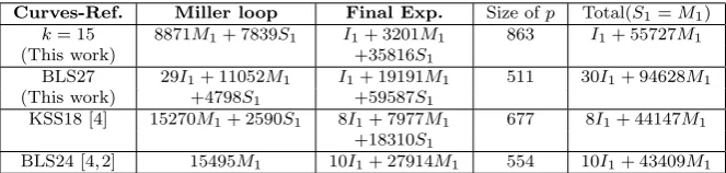
The following table 6 compares our results with previous results at the 192-bit security level.

Curves-Ref. Miller loop Final Exp. Size ofp Total(S1=M1)

k= 15 8871M1+ 7839S1 I1+ 3201M1 863 I1+ 55727M1

(This work) +35816S1

BLS27 29I1+ 11052M1 I1+ 19191M1 511 30I1+ 94628M1

(This work) +4798S1 +59587S1

KSS18 [4] 15270M1+ 2590S1 8I1+ 7977M1 677 8I1+ 44147M1

+18310S1

BLS24 [4, 2] 15495M1 10I1+ 27914M1 554 10I1+ 43409M1

Table 6 Comparison of the cost of the Miller loop and the final exponentiation at 192-bit security level.

8.3 New parameters and costs for pairings at the 256- bits security levels for

k= 27 andk= 24

– Case of k = 27. Following the recommendation from Table 4, we found the value x= 251_{+ 2}42_{+ 2}28_{+ 2}9_{+ 1. This gives a prime pof 1019 bits} and a prime factor of r of 883 bits. We proceed as described in section 6 to obtain the cost of the Miller loop and the final exponentiation. The Miller loop costs in this case 4(9M1+ 1I9+ 2S9+ 3M9) + 51(9M1+ 1I9+ 2S9+ 3M9) + 50S27+ 53M27. This is equal to 55I9+ 53M27+ 165M9+ 495M1+ 50S27+ 110S9. Using the arithmetic in Table 2, the overall cost is 55I1+ 21348M1+ 9660S1. Using the value of x given above, the final exponentiation costsI27+ 2(51S27+ 3M27) + 17(51S27+ 4M27) + 11M27+ 2IG_φ

3 (p9 ) andp, p

2_{, p}3_{, p}4_{, p}5_{, p}6_{, p}7_{, p}8_,2∗p9_{-Frobenius maps for a total cost} of the final exponentiationI1+ 19191M1+ 122337S1.

The cost for the casek= 24 are obtained with the parameter given in [4] and the formulas from [2]

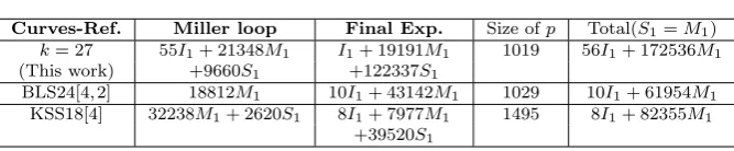
Curves-Ref. Miller loop Final Exp. Size ofp Total(S1=M1)

k= 27 55I1+ 21348M1 I1+ 19191M1 1019 56I1+ 172536M1

(This work) +9660S1 +122337S1

BLS24[4, 2] 18812M1 10I1+ 43142M1 1029 10I1+ 61954M1

KSS18[4] 32238M1+ 2620S1 8I1+ 7977M1 1495 8I1+ 82355M1

+39520S1

Table 7 Comparison of the cost of the Miller loop and the final exponentiation at 256-bit security level.

8.4 Comparison

To make a fair comparison of the results in tables 5, 6 and 7, we take note of the size of the base field. We consider implementations on 64-bit platform. Then following [2], aFpelement is represented with`= 1+log2(p) binary coefficients packed inn64 =d<sub>64</sub>`e64 bits processor words and aFp multiplication can be

implemented with approximately 2n264+n64 operations. We denote mc the

cost of a multiplication in the finite fieldFpwherepis ofcbits. For the Table

5 we have thatm461≈1.35m371. From this we see that, at the 128-bit security level, the total cost of computing the optimal ate pairing for elliptic curves withk= 15 is 19199m461making these curves faster than the well known BN curves but slower than the KSS16 curves found in [4] as the best one at the 128-bit security level. From Table 6 we have that the cost for computing the optimal ate pairing for curves withk= 15 is 166067m511 asm863≈2.98m511 . We conclude that at the 192-bit security level computing the optimal ate pairing is faster on elliptic curves with embedding degree k = 27 than on curves withk = 15 and in this case the BLS24 curves remain faster. At the 256-bit security level, we have that the BLS24 curves are the faster.

9 Conclusion

sub-group secure ordinary curves [6] and are not protected againstsmall-subgroup attacks[32]. However this is not a particular case of elliptic curves of odd em-bedding degree but it appears from [6] that most of such parameters that have been found for curves with even embedding degree such as BN12 curves [8], KSS16 curves [24] or BLS12 curves [7] do not satisfied these security prop-erties. As future work we could search for parameters to fulfill this security issue.

References

1. Diego F. Aranha, Laura Fuentes-Casta˜neda, Edward Knapp, Alfred Menezes, and Fran-cisco Rodr´ıguez-Henr´ıquez. Implementing pairings at the 192-bit security level. In

Pairing-Based Cryptography - Pairing 2012 - 5th International Conference, Cologne, Germany, May 16-18, 2012, Revised Selected Papers, pages 177–195, 2012.

2. Diego F. Aranha, Laura Fuentes-Casta˜neda, Edward Knapp, Alfred Menezes, and Fran-cisco Rodr´ıguez-Henr´ıquez. Implementing pairings at the 192-bit security level. In

Pairing-Based Cryptography - Pairing 2012 - 5th International Conference, Cologne, Germany, May 16-18, 2012, Revised Selected Papers, pages 177–195, 2012.

3. R. Avanzi, H. Cohen, C. Doche, G. Frey, T. Lange, K. Nguyen, and F. Vercauteren.

Handbook of Elliptic and Hyperelliptic curve Cryptography. Discrete Math. Aplli. Chap-man and Hall, 2006.

4. Razvan Barbulescu and Sylvain Duquesne. Updating key size estimations for pairings.

Journal of Cryptology, 2018.

5. Razvan Barbulescu, Pierrick Gaudry, Aurore Guillevic, and Fran¸cois Morain. Improv-ing NFS for the discrete logarithm problem in non-prime finite fields. InAdvances in Cryptology - EUROCRYPT 2015 - 34th Annual International Conference on the The-ory and Applications of Cryptographic Techniques, Sofia, Bulgaria, April 26-30, 2015, Proceedings, Part I, pages 129–155, 2015.

6. Paulo S. L. M. Barreto, Craig Costello, Rafael Misoczki, Michael Naehrig, Geovandro C. C. F. Pereira, and Gustavo Zanon. Subgroup security in pairing-based cryptography. InProgress in Cryptology - LATINCRYPT 2015 - 4th International Conference on Cryptology and Information Security in Latin America, Guadalajara, Mexico, August 23-26, 2015, Proceedings, pages 245–265, 2015.

7. Paulo S. L. M. Barreto, Ben Lynn, and Michael Scott. Constructing elliptic curves with prescribed embedding degrees. InSecurity in Communication Networks, Third International Conference, SCN 2002, Amalfi, Italy, September 11-13, 2002. Revised Papers, pages 257–267, 2002.

8. Paulo S. L. M. Barreto and Michael Naehrig. Pairing-friendly elliptic curves of prime order. In Selected Areas in Cryptography, 12th International Workshop, SAC 2005, Kingston, ON, Canada, August 11-12, 2005, Revised Selected Papers, pages 319–331, 2005.

9. I.F. Blake, G. Seroussi, and N.P. Smart. Advances in Elliptic Curves in Cryptography. London Mathematic Society, Cambridge University Press, (2005).

10. Dan Boneh and Matthew K. Franklin. Identity-based encryption from the Weil pairing. InAdvances in Cryptology - CRYPTO 2001, 21st Annual International Cryptology Conference, Santa Barbara, California, USA, August 19-23, 2001, Proceedings, pages 213–229, 2001.

11. Dan Boneh, Ben Lynn, and Hovav Shacham. Short signatures from the weil pairing.J. Cryptology, 17(4):297–319, 2004.

12. Clifford Cocks. An identity based encryption scheme based on quadratic residues. In

Cryptography and Coding, 8th IMA International Conference, Cirencester, UK, De-cember 17-19, 2001, Proceedings, pages 360–363, 2001.

14. Augusto Jun Devegili, Michael Scott, and Ricardo Dahab. Implementing cryptographic pairings over barreto-naehrig curves. InPairing-Based Cryptography - Pairing 2007, First International Conference, Tokyo, Japan, July 2-4, 2007, Proceedings, pages 197– 207, 2007.

15. Pu Duan, Shi Cui, and Choong Wah Chan. Special polynomial families for generating more suitable elliptic curves for pairing-based cryptosystems.IACR Cryptology ePrint Archive, 2005:342, 2005.

16. Ratna Dutta, Rana Barua, and Palash Sarkar. Pairing-based cryptographic protocols : A survey.IACR Cryptology ePrint Archive, 2004:64, 2004.

17. David Freeman, Michael Scott, and Edlyn Teske. A taxonomy of pairing-friendly elliptic curves. J. Cryptology, 23(2):224–280, 2010.

18. Laura Fuentes-Casta˜neda, Edward Knapp, and Francisco Rodr´ıguez-Henr´ıquez. Faster hashing toG2. InSelected Areas in Cryptography - 18th International Workshop, SAC

2011, Toronto, ON, Canada, August 11-12, 2011, Revised Selected Papers, pages 412– 430, 2011.

19. Vipul Goyal, Omkant Pandey, Amit Sahai, and Brent Waters. Attribute-based encryp-tion for fine-grained access control of encrypted data. InProceedings of the 13th ACM Conference on Computer and Communications Security, CCS 2006, Alexandria, VA, USA, Ioctober 30 - November 3, 2006, pages 89–98, 2006.

20. Robert Granger and Michael Scott. Faster squaring in the cyclotomic subgroup of sixth degree extensions. InPublic Key Cryptography - PKC 2010, 13th International Conference on Practice and Theory in Public Key Cryptography, Paris, France, May 26-28, 2010. Proceedings, pages 209–223, 2010.

21. Aurore Guillevic. Kim-barbulescu variant of the number field sieve to compute discrete logarithms in finite fields. In https://ellipticnews.wordpress.com/2016/05/02/kim- barbulescu-variant-of-the-number-field-sieve-to-compute-discrete-logarithms-in-finite-fields, ellipticnews, May 2016.

22. Florian Hess. Pairing lattices. InPairing-Based Cryptography - Pairing 2008, Second International Conference, Egham, UK, September 1-3, 2008. Proceedings, pages 18–38, 2008.

23. Florian Hess, Nigel P. Smart, and Frederik Vercauteren. The eta pairing revisited.IEEE Transactions on Information Theory, 52(10):4595–4602, 2006.

24. Ezekiel J. Kachisa, Edward F. Schaefer, and Michael Scott. Constructing brezing-weng pairing friendly elliptic curves using elements in the cyclotomic field.IACR Cryptology ePrint Archive, 2007:452, 2007.

25. Koray Karabina. Squaring in cyclotomic subgroups. Math. Comput., 82(281), 2013. 26. Taechan Kim and Razvan Barbulescu. Extended tower number field sieve: A new

com-plexity for the medium prime case. InCRYPTO (1), volume 9814 ofLecture Notes in Computer Science, pages 543–571. Springer, 2016.

27. Neal Koblitz and Alfred Menezes. Pairing-based cryptography at high security levels. InCryptography and Coding, 10th IMA International Conference, Cirencester, UK, December 19-21, 2005, Proceedings, pages 13–36, 2005.

28. Kristin E. Lauter, Peter L. Montgomery, and Michael Naehrig. An analysis of affine co-ordinates for pairing computation. InPairing-Based Cryptography - Pairing 2010 - 4th International Conference, Yamanaka Hot Spring, Japan, December 2010. Proceedings, pages 1–20, 2010.

29. Duc-Phong Le and Chik How Tan. Speeding up ate pairing computation in affine coordinates. InInformation Security and Cryptology - ICISC 2012 - 15th International Conference, Seoul, Korea, November 28-30, 2012, Revised Selected Papers, pages 262– 277, 2012.

30. Benoˆıt Libert and Jean-Jacques Quisquater. Identity based undeniable signatures. In

Topics in Cryptology - CT-RSA 2004, The Cryptographers’ Track at the RSA Confer-ence 2004, San Francisco, CA, USA, February 23-27, 2004, Proceedings, pages 112–125, 2004.

33. Xibin Lin, Changan Zhao, Fangguo Zhang, and Yanming Wang. Computing the ate pairing on elliptic curves with embedding degree k = 9. IEICE Transactions, 91-A(9):2387–2393, 2008.

34. Alfred Menezes, Palash Sarkar, and Shashank Singh. Challenges with assessing the impact of nfs advances on the security of pairing-based cryptography. Cryptology ePrint Archive, Report 2016/1102, 2016.

35. Victor S. Miller. The weil pairing, and its efficient calculation.J. Cryptology, 17(4):235– 261, 2004.

36. Nadia El Mrabet, Nicolas Guillermin, and Sorina Ionica. A study of pairing computation for elliptic curves with embedding degree 15.IACR Cryptology ePrint Archive, 2009:370, 2009.

37. Michael Scott, Naomi Benger, Manuel Charlemagne, Luis J. Dominguez Perez, and Ezekiel J. Kachisa. Fast hashing toG2 on pairing-friendly curves. InPairing-Based

Cryptography - Pairing 2009, Third International Conference, Palo Alto, CA, USA, August 12-14, 2009, Proceedings, pages 102–113, 2009.

38. Michael Scott and Aurore Guillevic. A new family of pairing-friendly elliptic curves. Cryptology ePrint Archive, Report 2018/193, 2018.

39. Frederik Vercauteren. Optimal pairings. IEEE Transactions on Information Theory, 56(1):455–461, 2010.

40. L.C. Washington. Elliptic Curves, Number Theory and Cryptography. Discrete Math .Aplli, Chapman and Hall, 2008.

41. Xusheng Zhang and Dongdai Lin. Analysis of optimum pairing products at high security levels. InProgress in Cryptology - INDOCRYPT 2012, 13th International Conference on Cryptology in India, Kolkata, India, December 9-12, 2012. Proceedings, pages 412– 430, 2012.

A Arithmetic in _Fp9

Leta=a0+a1v+a2v2∈Fp9 withai∈Fp3.

A.1 Cyclotomic inversion

We assume that a lies in the cyclotomic subgroup Gφ3(p3), so that a

p6+p3+1 _{= 1 i.e.}

a−1=ap6ap3. In order to computeap6ap3, we need the values ofvp3 andvp6. Butvp3= v3(p3−1)/3+1_=v3(p3−1)/3_{v= (v}3₎(p3−1)/3_{v= (7}1/3₎(p3−1)/3_vsincev3_{= 7}1/3_.

Letµ= (71/3₎(p3_−1)/3

; we haveµ6= 1 andµ3 _{= 1 so that µis a primitive cubic root of}

unity inFp3. We obtainvp 3

=µvandvp6_{= (v}p3₎p3_{= (µv)}p3_=µ(v)p3_=µµv=µ2_{v. We}

then haveap3=ap₀3+ap₁3vp3+ap₂3(v2)p3=a0+a1vp

3

+a2(v2)p

3

=a0+a1µv+a2µ2v2

andap6 _{= (a}p3₎p3 _=a

0+a1(µv)p

3

+a2(µ2v2)p

3

=a0+a1µ2v+a2µ4v2. So that when

usingv3_{= 7}1/3_andφ

3(µ) =µ2+µ+ 1 = 0, we finally have:

ap6ap3= (a20−a1a271/3) + (a2271/3−a0a1)v+ (a21−a0a2)v2

This costs 3M3+ 3S3= 18M1+ 15S1with additional additions.

A.2 Frobenius operators

Thepi_{−Frobenius is the mapπ}i_:

Fp9 →Fp9, a7→ap

i

. Leta∈Fp9,a=a0+a1v+a2v2

withai ∈ Fp3 thenπ(a) =ap₀+ap₁vp+ap₂(v2)p. Nowa0 ∈ Fp3 can be written asa0 =

We haveup _=u3(p−1)/3+1 _{= (u}3₎(p−1)/3_{u = 7}(p−1)/3_{u and since 7 is not a cube in} Fp,

7(p−1)/3_{6= 1. Letα= 7}(p−1)/3_{thenα6= 1 andα}3_{= 1; it means thatαis a primitive cubic}

root of unity inFpandup=αu. Thereforeap0=g0+g1up+g2(u2)p=g0+g1αu+g2α2u2

and similarlyap₁=g3+g4up+g5(u2)p=g3+g4αu+g5α2u2and

ap2 =g6+g7up+g8(u2)p=g6+g7αu+g8α2u2. Now for the computation ofvpobserve

thatvp_=v3(p−1)/3+1_{= (v}3₎(p−1)/3_{v= (7}1/3₎(p−1)/3_{v= 7}(p−1)/9_{vso that ifβ= 7}(p−1)/9

then we haveβ6= 1,β3 _{= 7}(p−1)/3_{=α6= 1, β}9 _{= 1. Thusβis a primitive ninth root of}

unity inFpandvp=βv.

Finallyap_=g

0+g1αu+g2α2u2+(g3β+g4αβu+g5α2βu2)v+(g6β2+g7αβ2u+g8α2β2u2)v2

and the following algebraic relations:α=β3_,αβ=β4_,αβ2_=β5_,α2_β=β7_,α2_β2 _=β8

yield toap_{= (g}

0+g1β3u+g2β6u2) + (g3β+g4β4u+g5β7u2)v+ (g6β2+g7β5u+g8β8u2)v2.

The cost ofp-Frobenius: 8M1. This is the same as the cost ofp2, p4, p5, p7andp8-Frobenius.

For thep3_{-Frobenius operator, observe from A.1 thatv}p3 _{=µv. Then}

ap3_=a

0+a1µv+a2µ2v2= (g0+g1u+g2u2) + (g3+g4u+g5u2)µv+ (g6+g7u+g8u2)µ2v2.

Ast=µ2_{is precomputed; we finally have}

ap3_{= (g}

0+g1u+g2u2) + (g3µ+g4µu+g5µu2)v+ (g6t+g7tu+g8tu2)v2.

The cost ofp3_{-Frobenius: 6M}

1. This is the same as the cost ofp6-Frobenius.

B Arithmetic inFp27

B.1 Cyclotomic inversion

We follow the same procedure as in A.1. The elementa=a0+a1w+a2w2∈Fp27withai∈

Fp9 in the cyclotomic subgroupGφ3(Fp9)satisfiesa

p18+p9+1_{= 1 so thata}−1_=ap18_ap9_.

In order to computeap18_ap9_{, we need the values ofw}p9 _andwp18_{. We have}

wp9 _=w3(p9−1)/3+1_=w3(p9−1)/3_{w= (w}3₎(p9−1)/3_{w= (7}1/9₎(p9−1)/3_wsincew3_{= 7}1/9_.

Let σ = (71/9₎(p9−1)/3 _{then σ 6= 1 and σ}3 _{= 1. Hence σ is a primitive cubic root}

of unity in Fp9 i.e. φ3(σ) = 0. We obtain wp

9

= σw and we now compute wp18 as

wp18_{= (w}p9₎p9_{= (σw)}p9 _=σ(w)p9_=σσw=σ2_w.

ap9_=a

0+a1wp

9

+a2(w2)p

9

=a0+a1σw+a2σ2w2 and

ap18 = (ap9

)p9

=a0+a1(σw)p

9

+a2(σ2w2)p

9

=a0+a1σ2w+a2σ4w2. After expanding

and reducing usingw3= 71/9andφ3(σ) =σ2+σ+ 1 = 0 we obtain

ap18ap9= (a20−a1a271/9) + (a2271/9−a0a1)w+ (a21−a0a2)w2

The computation costs 3(36M1) + 3(25S1) = 108M1+ 75S1.

B.2 Frobenius operators

Thepi_{−Frobenius is the mapπ}i_:

Fp27 →Fp27, a7→ap

i

. Leta=a0+a1w+a2w2 with

ai∈Fp9 an element ofFp27.

π(a) =ap _{= (a}

0+a1w+a2w2)p=ap₀+a₁pwp+ap₂(w2)p. The elementa0 ∈Fp9 can be written asa0= (h0+h1u+h2u2) + (h3+h4u+h5u2)v+ (h6+h7u+h8u2)v2,hi∈Fp.

We haveap₀= (h0+h1u+h2u2+ (h3+h4u+h5u2)v+ (h6+h7u+h8u2)v2)p,hpi =hi.

up _{= u}3(p−1)/3+1 _{= (u}3₎(p−1)/3_{u = 7}(p−1)/3_{u. Since 7 is not a cube in}

Fp, we have

α= 7(p−1)/3 _{α6= 1 andα}3 _{= 1. It means thatαis a primitive cubic root of unity in} Fp

andup_=αu.vp_=v3(p−1)/3+1_{= (v}3₎(p−1)/3_{v= (7}1/3₎(p−1)/3_{v= 7}(p−1)/9_v.

We haveβ= 7(p−1)/9_{6= 1 andβ}9_{= 1. Thusβis a primitive ninth root of unity in} Fpand

Thusγis a primitive twenty-seventh root of unity inFpandwp=γw.

ap₀= ((h0+h1u+h2u2) + (h3+h4u+h5u2)v+ (h6+h7u+h8u2)v2)p

= (h0+h1up+h2(u2)p) + (h3+h4up+h5(u2)p)vp+ (h6+h7up+h8(u2)p)(v2)p

= (h0+h1αu+h2α2u2) + (h3+h4αu+h5α2u2)βv+ (h6+h7αu+h8α2u2)β2v2

= (h0+h1αu+h2α2u2)+(h3β+h4αβu+h5α2βu2)v+(h6β2+h7αβ2u+h8α2β2u2)v2.

ap₁= (h9+h10u+h11u2) + (h12+h13u+h14u2)v+ (h15+h16u+h17u2)v2)p

= (h9+h10up+h11(u2)p)+(h12+h13up+h14(u2)p)vp+(h15+h16up+h17(u2)p)(v2)p

= (h9+h10αu+h11α2u2)+(h12+h13αu+h14α2u2)βv+(h15+h16αu+h17α2u2)β2v2

= (h9+h10αu+h11α2u2) + (h12β+h13αβu+h14α2βu2)v+ (h15β2+h16αβ2u+

h17α2β2u2)v2.

ap₂= (h18+h19u+h20u2) + (h21+h22u+h23u2)v+ (h24+h25u+h26u2)v2)p

= (h18+h19up+h20(u2)p)+(h21+h22up+h23(u2)p)vp+(h24+h25up+h26(u2)p)(v2)p

= (h18+h19αu+h20α2u2)+(h21+h22αu+h23α2u2)βv+(h24+h25αu+h26α2u2)β2v2.

= (h18+h19αu+h20α2u2) + (h21β+h22αβu+h23α2βu2)v+ (h24β2+h25αβ2u+

h26α2β2u2)v2.

π(a) = (a0+a1w+a2w2)p=ap0+a

p

1wp+a

p

2(w2)p=a

p

0+a

p

1γw+a

p

2γ2w2

= (h0+h1αu+h2α2u2) + (h3β+h4αβu+h5α2βu2)v+ (h6β2 +h7αβ2u+

h8α2β2u2)v2+

((h9+h10αu+h11α2u2) + (h12β+h13αβu+h14α2βu2)v+ (h15β2+h16αβ2u+

h17α2β2u2)v2)γw+ ((h18+h19αu+h20α2u2) + (h21β+h22αβu+h23α2βu2)v+

(h24β2+h25αβ2u+h26α2β2u2)v2)γ2w2.

We have these following algebraic relations:α=β3,αβ =β4,αβ2 =β5,α2β =β7 and α2_β2_=β8_{. Therefore}

π(a) = ((h0+h1β3u+h2β6u2) + (h3β+h4β4u+h5β7u2)v+ (h6β2+h7β5u+h8β8u2)v2)+

((h9γ+h10β3γu+h11β6γu2)+(h12βγ+h13β4γu+h14β7γu2)v+(h15β2γ+h16β5γu+

h17β8γu2)v2)w+ ((h18γ2+h19β3γ2u+h20β6γ2u2) + (h21βγ2 +h22β4γ2u+

h23β7γ2u2)v+

(h24β2γ2+h25β5γ2u+h26β8γ2u2)v2)w2.

The following values are precomputed:λ0 = β2,λ1 =β3,λ2 =β4,λ3 =β5,λ4 = β6,

λ5 = β7,λ6 =β8,λ7 =γ2 ,λ8 = βγ,λ9 = λ0γ,λ10 = λ1γ,λ11 = λ2γ,λ12 = λ3γ,

λ13 = λ4γ,λ14 =λ5γ,λ15 =λ6γ,λ16 =λ0λ7,λ17 =λ1λ7,λ18= λ2λ7,λ19 =λ3λ7,

λ20=λ4λ7,λ21=λ5λ7,λ22=λ6λ7.λ23=βλ7.

Thusπ(a) = ((h0+h1λ1u+h2λ4u2) + (h3β+h4λ2u+h5λ5u2)v+ (h6λ0+h7λ3u+

h8λ6u2)v2) + ((h9γ+h10λ10u+h11λ13u2) + (h12λ8+h13λ11u+h14λ14u2)v+

(h15λ9+h16λ12u+h17λ15u2)v2)w+ ((h18λ7+h19λ17u+h20λ20u2) + (h21λ23+

h22λ18u+h23λ21u2)v+ (h24λ16+h25λ19u+h26λ22u2)v2)w2.

The cost of p-Frobenius: 26M1+ 18a. This is also equal to the cost ofp2, p4, p5, p7, p8

Frobenius

For thep9_{Frobenius operator, observe from B.1 thatw}p9_{=σw. Then}

ap9_=a

0+a1σw+a2σ2w2= ((h0+h1u+h2u2) + (h3+h4u+h5u2)v+ (h6+h7u+

h8u2)v2) + ((h9+h10u+h11u2) + (h12+h13u+h14u2)v+ (h15+h16u+

h17u2)v2)σw+

((h18+h19u+h20u2) + (h21+h22u+h23u2)v+ (h24+h25u+h26u2)v2)σ2w2.

We then haveap9= ((h0+h1u+h2u2) + (h3+h4u+h5u2)v+ (h6+h7u+h8u2)v2)+

((h9σ+h10σu+h11σu2)+(h12σ+h13σu+h14σu2)v+(h15σ+h16σu+

h17σu2)v2)w+ ((h18σ2+h19σ2u+h20σ2u2) + (h21σ2+h22σ2u+

h23σ2u2)v+ (h24σ2+h25σ2u+h26σ2u2)v2)w2.

Ass=σ2 _{is precomputed; we havea}p9_{= ((h}

0+h1u+h2u2) + (h3+h4u+h5u2)v+

(h6+h7u+h8u2)v2) + ((h9σ+h10σu+h11σu2) + (h12σ+h13σu+h14σu2)v+ (h15σ+

h16σu+h17σu2)v2)w+ ((h18s+h19su+h20su2) + (h21s+h22su+h23su2)v+ (h24s+

h25su+h26su2)v2)w2.