Comparative study on performance of 2D Image Processing Algorithm implemented in parallel and sequential models

(1)

IJEDR1401188

International Journal of Engineering Development and Research (www.ijedr.org)

1050

Comparative study on performance of 2D Image

Processing Algorithm implemented in parallel and

sequential models

1

Balaji Vengatesh M.,

2

Joseph Raymond V

1_{M.Tech. Scholar,}2_{Assistant Professor}

Department of Information Technology, SRM UNIVERSITY, Chennai, India

1_{[email protected],}2_{[email protected]}

________________________________________________________________________________________________________

Abstract—This paper deals with the Parallel Implementation of an Image Processing Algorithm and comparing the same with the sequential Implementation of the algorithm and demonstrate the Increase in speeds through Hardware rather optimizing the code for the same. We chose the Canny Edge Detection algorithm that aims at identifying points in a digital image where the image brightness changes sharply. The paper also deals with parallel Implementation on CUDALink, A Library or link provided by Wolfram Mathematica 9,which allows mathematica to use CUDA parallel computing architecture developed by NVIDIA to be used by Mathematica. We use the Mathematica’s Inbuilt Edge Detection function that runs on the CPU to compare with our parallel Implementation on the GPU. The comparison further speaks more on the quality of edges and also the running times of both the algorithm. The GPU we use here is the NVIDIA GTX 560 Ti Edition.

Index Terms—FPGA, CUDA, GPU, Mathematica, OpenCV

________________________________________________________________________________________________________

I. INTRODUCTION

GPU’s are originally intended for graphics applications such as games. But during the 2000’s programmers started using a version of Open GL for developing General purpose applications that are mainly intended to run on a computer without a graphics processor. Early in the year 2005 NVIDIA came up with the development of new framework for GPGPU applications such as image processing. The new framework was named CUDA. The present version is CUDA 5.5.

In the year 1985 John canny came up with an idea of an efficient algorithm for Edge detection that is computationally possible and efficient[1].Since then many edge detection algorithms were under use one such was step edge detector used in computer vision systems. Edge detection has wide variety of applications, hence it becomes nessacary for one to develop a efficient method for this. The edge detection process serves to simplify the analysis of images by drastically reducing the amount of data to be processed, while at the same time preserving useful structural information about object

boundaries[1].

The paper also deals with parallel programming of the edge detection algorithm. The most popular parallel programming language is the OPEN MP. Similar to this NVIDIA developed CUDA C a programming framework based on C.The main advantage of going to a GPU is it performs highly specialized tasks whereas CPU is a general purpose processor[2]. The programming and implementation are made easy with wolfram Mathematica, which is a computational software program used in many scientific, engineering, mathematical and computing fields, based on symbolic mathematics[3].

II. BACKGROUND

A. NVidia Compute Unified Device Architecture

Developing optimized programs using CUDA demands a good understanding of the GPGPU architecture abstraction and programming paradigm. The creation, scheduling and completion of all threads in CUDA are controlled by the GPU hardware [4]. The threads are organized hierarchically into grids of thread blocks. Each active block is divided into groups of threads called warps. A warp has 32 threads and is scheduled with other warps in a multiprocessor. Each multiprocessor has thread processors and an execution controller.

All thread processors in a warp execute the same instruction simultaneously, so that the maximum efficiency is achieved when all 32 threads in a warp have the same execution flow. Any flow control instruction (if, switch, do, for, while) might increase the execution time by dividing the warp into divergent execution flows. When this happens, the warp is divided into groups of threads with the same execution flow, and the execution of the thread groups of a warp is serialized by the multiprocessor. Warps that have their execution serialized are called divergent warps.

(2)

IJEDR1401188

1051

and Constant caches. Each multiprocessor also has an additional memory shared by all threads: the shared memory, and each thread processor in a multiprocessor owns a register set.

Hiding memory access latency is possible by using the shared memory as a cache [9], since it is almost as fast as the processor registers. Texture and Constant caches are also efficient to optimize global memory access, because of their prefetch mechanism. Therefore this work used linear Texture cache for almost all read-only global memory accesses.

B. Wolfram Mathematica CUDALink

Mathematica is a computational software program used in many scientific, engineering, mathematical and computing fields, based on symbolic mathematics. It was conceived by Stephen Wolfram and is developed by Wolfram Research of Champaign, Illinois[5]. Some features include

1. Automatic translation of English sentences into Mathematica code 2. Elementary mathematical function library

3. Special mathematical function library

4. Matrix and data manipulation tools including support for sparse arrays

5. Tools for connecting to DLLs. SQL, Java, .NET, C++, Fortran, CUDA, OpenCL and http based systems

In this work we are highly interested the fifth feature described above. Mathematica also provides useful functionalies to convert the given C code into CUDA C, switchover the codes between CUDA and OpenCL. Our work is centered around CUDALink, Provided by Mathematica. CUDALink allows Mathematica to use the CUDA parallel computing architecture on Graphical Processing Units (GPUs). It contains functions that use CUDA-enabled GPUs to boost performance in a number of areas, such as linear algebra, financial simulation, and image processing. CUDALink also integrates CUDA with existing Mathematica

development tools, allowing a high degree of automation and control.[6]The following are the steps to use CUDALink for running a CUDA code. we use a specific version of Mathematica 9.0. Fig 1.1 depicts the general CUDA programming approach

1. Develop the code in a separate notepad, provided by windows 7 or use the notebook in Mathematica to develop code 2. Assign variables for code, if code is developed in a notepad use Filename Join[] function

3. Assign variables for separate functions. 4. Compile and Run the Mathematica code.

Fig2.1 General CUDA Programming Approach with Visual Studio Figure 1.1 shows the typical cycle of a CUDA program[6].

1. Allocate memory of the GPU. GPU and CPU memory are physically separate, and the programmer must manage the allocation copies.

2. Copy the memory from the CPU to the GPU.

3. Configure the thread configuration: choose the correct block and grid dimension for the problem. 4. Launch the threads configured.

5. Synchronize the CUDA threads to ensure that the device has completed all its tasks before doing further operations on the GPU memory.

6. Once the threads have completed, memory is copied back from the GPU to the CPU. 7. The GPU memory is freed.

(3)

IJEDR1401188

1052

III. CANNY ALGORITHM

The Canny edge detection algorithm begins with a Gaussian filtering to smooth the input image and reduce false edges detection. It then computes the image’s gradient magnitude and direction through first or second order derivative operators. First order derivatives like Sobel filter are simpler and faster, but second order derivative operators present better results with a better signal-to-noise ratio and sub-pixel resolution [1]. One commonly used second order derivative computation is based on differential geometry [1], [1]. The next step is called Non-Maximum Suppression (NMS) and consists of setting all pixels that are not maximum at the gradient’s direction on a neighborhood to zero. Remaining pixels are subjected to a double threshold hysteresis process to define the final edge pixels.

A. Gaussian Smoothing

It is inevitable that all images taken from a camera will contain some amount of noise. To prevent that noise is mistaken for edges, noise must be reduced. Therefore the image is first smoothed by applying a Gaussian filter. The kernel of a Gaussian filter with a standard deviation of σ = 1.4 is shown in Equation (1). The effect of smoothing the test image with this filter is shown in Figure 3.1.

Fig3.1 Image before and after smoothing

B. First Order Derivative Sobel Filter

The Canny algorithm basically finds edges where the grayscale intensity of the image changes the most. These areas are found by determining gradients of the image. Gradients at each pixel in the smoothed image are determined by applying what is known as the Sobel-operator. First step is to approximate the gradient in the x- and y-direction respectively by applying the kernels shown in Equation (2).

C. Second Order Derivative Gradient

The gradient magnitudes (also known as the edge strengths) can then be determined as an Euclidean distance measure by applying the law of Pythagoras as shown in Equation (3). It is sometimes simplified by applying Manhattan distance measure as shown in Equation (4) to reduce the computational complexity. The Euclidean distance measure has been applied to the test image. The computed edge strengths are compared to the smoothed image in Figure 3.2.

(4)

IJEDR1401188

1053

Fig3.2 The Gradient magnitudes in the smoothed image is shown

D. Non-maximum Suppression

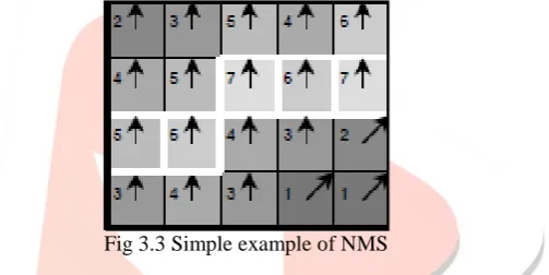
The purpose of this step is to convert the “blurred” edges in the image of the gradient magnitudes to “sharp” edges. Basically this is done by preserving all local maxima in the gradient image, and deleting everything else. The algorithm is for each pixel in the gradient image

1. Round the gradient direction to nearest 45., corresponding to the use of an 8-connected neighbourhood.

2. Compare the edge strength of the current pixel with the edge strength of the pixel in the positive and negative gradient direction. I.e. if the gradient direction is north (theta = 90.), compare with the pixels to the north and south.

3. If the edge strength of the current pixel is largest; preserve the value of the edge strength. If not, suppress (i.e. remove) the value.

Fig 3.3 Simple example of NMS

A simple example of non-maximum suppression is shown in Figure 3.3. Almost all pixels have gradient directions pointing north. They are therefore compared with the pixels above and below. The pixels that turn out to be maximal in this comparison are marked with white borders. All other pixels will be suppressed. Figure 3.4 shows the effect on the test image.

Fig 3.4 Effect of NMS on Test Image

E. Hysteresis Thresholding

(5)

IJEDR1401188

1054

Fig 3.5 Double Threshold Image

Strong edges are interpreted as “certain edges”, and can immediately be included in the final edge image. Weak edges are included if and only if they are connected to strong edges. The logic is of course that noise and other small variations are unlikely to result in a strong edge (with proper adjustment of the threshold levels). Thus strong edges will (almost) only be due to true edges in the original image. The weak edges can either be due to true edges or noise/color variations. The latter type will probably be distributed independently of edges on the entire image, and thus only a small amount will be located adjacent to strong edges. Weak edges due to true edges are much more likely to be connected directly to strong edges.

Edge tracking can be implemented by BLOB-analysis (Binary Large OBject). The edge pixels are divided into connected BLOB’s using 8-connected neighbourhood. BLOB’s containing at least one strong edge pixel are then preserved, while other BLOB’s are suppressed. The effect of edge tracking on the test image is shown in Figure 3.6.

Fig 3.6 Hysteresis and Final output

IV. IMPLEMENTATION AND RESULTS

A.WorkItems:

In order to Implement the canny algorithm we choose a 512x512 Lena Image in GIF format acceptable by mathematica The Implementation can also be done on various other Image formats specified by mathematica. The work item before processing is shown in fig 4.1

(6)

IJEDR1401188

1055

B.Implemtation

First we enable the CUDALink with Needs statement of Mathematica [3]. Then we import the note pad file with the desired filename.cuda by using filename join and store it in a memory variable of cuda. Then we declare different mathematica variables to load the kernels using CUDAFunctionLoad method of mathematica. The kernels are compiled with a C compiler. We use Visual studio 2010 C compiler linked with mathematica tool. The Image is imported using the inbuilt import function in mathematica. Memory is loaded and allocated for CUDAmemoryload and CUDAmemoryallocate functions for the declared variables in the kernel. Execution is done by calling memory variables in mathematica. The steps of execution is shown here in fig 4.2

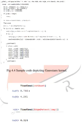
By following the steps in fig 4.2 any image processing algorithm can be implemented in Mathematica. Image[SOURCE] method is used for viewing images over mathematica’s workspace depicited in fig 4.3. The code snippet for Canny edge detection in CUDA C is shown in fig 4.4, As stated before we use windows text editor for programming in CUDA C. The file is saved as .cu extension.

Fig 4.4 Sample code depicting Gaussianx kernel.

C.Results

Fig 4.3 mathematica workspace

(7)

IJEDR1401188

1056

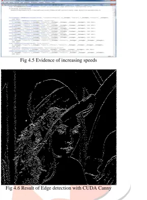
Fig 4.5 Evidence of increasing speeds

Fig 4.6 Result of Edge detection with CUDA Canny

REFERENCES

[1] John Canny,A computational approach to edge detection IEEE TRANSACTIONS ON PATTERN ANALYSIS AND MACHINE INTELLIGENCE, VOL. PAMI-8, NO. 6, NOVEMBER 1986

[2] Yuancheng “Mike” Luo and Ramani Duraiswami “canny edge detection on NVIDIA CUDA” [3] http://en.wikipedia.org/wiki/MathematicaK. Elissa, “Title of paper if known,” unpublished.

[4] Luis H.A. Lourenc¸o, Daniel Weingaertner and Eduardo Todt Efficient implementation of Canny Edge DetectionFilter for ITK using CUDA Informatics Department, Universidade Federal do Paran´aCuritiba, Brazil

[5] Canny Edge Detection Tutorial by jing juck jang, Tsingshua university, Mainland China [6] R. Palomar, J. M. Palomares, J. M. Castillo, J. Olivares, and J. G´omez-

[7] Luna, “Parallelizing and optimizing lip-canny using nvidia cuda,” ser. [8] IEA/AIE’10. Berlin, Heidelberg: Springer-Verlag, 2010, pp. 389–398. [9] V. Podlozhnyuk, “Image convolution with cuda,” June 2007.

[10]“Insight segmentation and registration toolkit,” 1999. [Online].Available: http://www.itk.org [11] W.-K. Jeong, “Cudaitk,” 2007. [Online]. Available: http://www.cs.utah. edu/_wkjeong/

[12]R. Beare, M. Kuiper, D. Micevski, C. Share, L. Parkinson, and P. Ward, “Cuda insight toolkit,” 2010. [Online]. Available: