OPTIMIZING INCLUDED ANGLE OF SYMMETRICAL V-DIPOLES FOR HIGHER DIRECTIVITY USING
BACTERIA FORAGING OPTIMIZATION ALGORITHM
B. B. Mangaraj
Department of Electronics & Telecommunication Engg. University College of Engineering
Burla, Sambalpur-768018, India
I. S. Misra
Department of Electronics and Tele-Communication Engg. Jadavpur University
Kolkata-700032, India
A. K. Barisal
Department of Electronics & Telecommunication Engg. University College of Engineering
Burla, Sambalpur-768018, India
Abstract—Recently the social foraging behavior of E. coli bacteria
1. INTRODUCTION
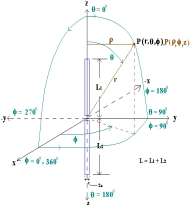
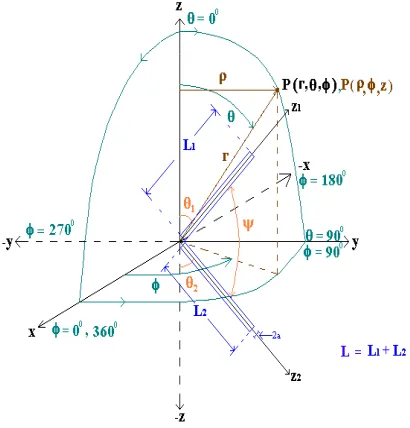
In this paper, firstly Bacteria Foraging Algorithm (BFA) has been explained briefly which is our goal to apply in the antenna problem. Both straight and V dipoles antennas or antenna are considered as the test objects and for comparison purpose. The structural details for both are depicted in Figure 1 and Figure 2. Straight dipole is considered as a simple case while V-dipole as a complex structure for the application of BFA. Both dipoles are analyzed and equations are derived using Method of Moments [1–3] to get current distribution on the antenna surface. We have considered only symmetrical V-dipole antennas for the analysis that can be easily extended for asymmetrical antenna also.
Figure 1. Straight dipole in rectangular, cylindrical & spherical co-ordinate system.
Figure 2. V-dipole in rectangular, cylindrical & spherical co-ordinate system.
Bacteria Foraging technique [4–7] is gaining importance in the optimization problems. Because,
1. Philosophy say Biology provides highly automated, robust and effective organism
2. Search strategy of bacteria is salutatory (like common fish) in nature
3. Bacteria can sense, decide and act to adopt social foraging (foraging in groups).
Above all Search and optimal foraging decision-making of animals can be used for solving engineering problems. To perform social foraging an animal needs communication capabilities and it gains advantages that can exploit essentially the sensing capabilities of the group, so that the group can gang-up on larger prey, individuals can obtain protection from predators while in a group, and in a certain sense the group can forage a type of collective intelligence.
Taking straight and V-dipole antenna structure as test systems; the principle of operation and complete analysis has been described. In the analysis part the electric field, magnetic field, input impedance and directivity in dB have been derived for both type of dipoles. All these parameters are function of included angle in case of a V dipole. The directivity (DR) is the Cost function of the V dipole, which is to be maximized. As the directivity is a function of included angle, BFA is applied to search the best included angle to realize the maximum directivity. The BFA is usually used to minimize the Cost function of the system. To achieve this, a fitness function FT (ψ) has been formulated out of this Cost function of the dipole system in such a way that when fitness function is minimized, the Cost function gets maximized. This fitness function becomes the COST function for bacteria in BFA. Finally, optimization of included angle using BFA is shown after getting minimized COST function. In the result section a comparative statement for both dipoles are given.
2. BACTERIA FORAGING OPTIMIZATION: A BRIEF OVERVIEW
1) Chemotaxis: This process is achieved through swimming and tumbling. Depending upon the rotation of the flagella in each bacterium, it decides whether it should move in a predefined direction (swimming) or an altogether different direction (tumbling), in the entire lifetime of the bacterium. To represent a tumble, a unit length random direction, φ(j) say, is generated; this will be used to define the direction of movement after a tumble. In particular
θi(j+ 1, k, l) =θi(j, k, l) +C(i)φ(j) (1)
where, θi(j, k, l) represents the ith bacterium at jth chemotactic
kth reproductive, and lth elimination and dispersal step. C(i) is the size of the step taken in the random direction specified by the tumble. “C” is termed as the “run length unit.”
2) Swarming: It is always desired that the bacterium that has searched the optimum path of food should try to attract other bacteria so that they reach the desired place more rapidly. Swarming makes the bacteria congregate into groups and hence move as concentric patterns of groups with high bacterial density. Mathematically, swarming can be represented by
Jcc(θ, P(j, k, l)) = S
i=1
Jcci θ, θi(j, k, l)
=
S
i=1
−dattractexp
−ωattract p
m=1
θm−θim
2
+
S
i=1
hrepelentexp
−ωrepelent p
m=1
θm−θim
2
(2)
whereJcc(θ, P(j, k, l)) is the cost function value to be added to the
actual cost function to be minimized to present a time varying cost function. “S” is the total number of bacteria. “p” is the number of parameters to be optimized that are present in each bacterium.
dattract, ωattract, hrepelent, and ωrepelent are different coefficients
that are to be chosen judiciously.
gradually by consumption of nutrients or suddenly due to some other influence. Events can kill or disperse all the bacteria in a region. They have the effect of possibly destroying the chemotactic progress, but in contrast, they also assist it, since dispersal may place bacteria near good food sources. Elimination and dispersal helps in reducing the behavior of stagnation (i.e., being trapped in a premature solution point or local optima). The detailed mathematical derivations as well as theoretical aspect of this new concept are presented in [5, 6].
3. PROBLEM STATEMENT
Problem: To increase the radiation characteristic, V-dipole has been considered and analyzed. The parameter directivity of the V-dipole is maximized by searching best included angle with the help of BFA. The result is also compared with similar length straight dipole. In literature many complicated structures have been analyzed to get higher directivity. In this paper, our attempt is to analyze a simple structure to get higher directivity by applying BFA.
A. Test System
In this paper, two structures, one straight dipole and one V-dipole of equal length, each of radius = 0.001λhave been considered as shown in Figure 1 and Figure 2, λ is the wavelength of the signal applied at feed point. If spherical co-ordinate system is considered then the straight dipole is along thez-axis and feed point is at the center of the co-ordinate system. The feed system along with the signal source is symmetrical to the plane (θ= 0◦andφ= 90◦). The V-dipole has been considered in the same way but one half makes an angleθ1with positive
z-axis and other half makes an angle θ2 with negative z-axis. This means V-dipole has an included angle (ψ), where ψ+θ1+θ2 = 180◦. Since symmetrical dipole system has been emphasized, so for V-dipole
θ1=θ2 and ψ=π−2θ1 =π−2θ2.
B. Operating Principle of the Intended Structure
C. Optimal Directivity or Directive Gain (ODG): Problem Formulation
The ODG problem is a nonlinear optimization problem, the solution of which determines the optimal settings of included angle. Hence, the problem is to solve a set of nonlinear equations describing the optimal solution of dipole radiating system.
Hallen’s integral equation has been formulated for a center-fed cylindrical straight dipole and V-dipole by considering unknown current distribution and applied RF signal. To find the current distribution and input impedance Hallen’s equation is solved using Method of Moments [7]. Here each arm of the structures is treated separately and finally their responses are added vectorially to get the desired expression. The current distribution is an unknown quantity and is to be found out such that the resultant tangential electric field cancels the applied field over the feed-gap and equals zero along the rest of the surface of the perfectly conducting structure. When the currents and boundary conditions of the electromagnetic problem to be solved are known, both the electric and magnetic fields can be found. This is usually done with the help of vector potential. The current density and vector potential are related as follows.
A(r) = µ
v
J(r)exp (−jk|r−r
|)
4π|r−r| dv
(3)
H(r) = 1
µ∇ ×A(r
) (4)
E(r) = −jωA(r)−j∇∇.A(r )
ωµε (5)
Considering thin wire approximation, the vector potential for upper arm length in cylindrical co-ordinate system can be written as
Az1 =µ
2π
0
L1
0 ˆ
zI(z
1) 2πa
exp(−jkR) 4πR dz
1adϕ (6)
whereR=|r−r|= [(z1−z1) +a2]1/2.
Solving the boundary condition for electric field and considering feed gap negligibly small, the Hallen’s integral equation for upper arm length is expressed as given below.
k2+ ∂ 2
∂z2 1
Solving the above differential Equation (7) and finding unknown constants of the solution by considering various approximations for vector potential, the solved equation is given as
L1
0
I(z1)G(z1, z1)dz1 =−
j
2η sink|z1|+A1coskz1 (8)
where bothz1 and z1 are constrained to (0,L1) and where
G(z1, z1) = exp
−jka2+ (z1−z1)2 1/2
4π[a2+ (z
1−z1)2]1/2
(9)
Using Method of Moments the Equation (8) can be written as
N
n=1
I(n)
n∆
(n−1)∆
G(m−0.5)∆, z1dz1 −A1cosk[(m−0.5)∆]
= − j
2ηcosθ1sink[(m−0.5)∆] (10)
Writing Equation (10) in matrix form
G1,1 G1,2 · · G1,N−1 −coskz1,1
G2,1 G2,2 · · G1,N−1 −coskz1,2
· · · · · ·
· · · · · ·
GN,1 · · · GN,N−1 −coskz1,m
I1 I2 · IN−1
A2 = −j
2ηcosθ1sink|z1,1|
−j
2ηcosθ1sink|z1,2|
· · −j
2ηcosθ1sink|z1,m|
(11)
Similarly, for the lower half arm one can find out another matrix as given below.
G1,1 G1,2 · · G1,N−1 −coskz2,1
G2,1 G2,2 · · G2,N−1 −coskz2,2
· · · · · ·
· · · · · ·
GN,1 · · · GN,N−1 −coskz2,m
I1 I2 · IN−1
A2 = j
2ηcos(ψ+θ1) sink|z2,1| j
2ηcos(ψ+θ1) sink|z2,2|
· ·
j
2ηcos(ψ+θ1) sink|z2,m|
(12)
phase. Adding both the matrix equation will generate Equation (13).
G1,1 G1,2 · · G1,N−1 −coskz2,1
G2,1 G2,2 · · G2,N−1 −coskz2,2 · · · · · · · · · · · ·
GN,1 · · · GN,N−1 −coskz2,m
I1 I2 ·
IN−1
A1 = j
4η{cos(ψ+θ1) sink|z2,1| −cosθ1sin|z1,1|} j
4η{cos(ψ+θ1) sink|z2,2| − cosθ1sin|z1,2|}
· ·
j
4η{cos(ψ+θ1) sink|z2,m| −cosθ1sin|z1,m|}
(13)
Manipulating above matrix equation, unknown current distribution can be found out.
Once the current distribution is known then input impedance, E and H field and Directivity can be found out as given below.
Zin=
1
I1(l)
(14)
In case of the straight dipole the far field electric component can be written as [4],
Eθ = jη
kIme−jkr
4πr sinθ
0
−L2
sinkL2+z
e+jkzcosθdz
+ +L1
0
sinkL1−z
e+jkzcosθdz
(15)
But in case of V-dipole, there will be two electric components, due to the included angle between the arms. Upper arm has been considered in the direction ofz1 and lower arm has been considered in the direction ofz2.
The far field electric component for the V-dipole can be written as
Eθ = jk η
4πsinθ
L1
0
Imsin{k(L1−z1)}
r1
e−jkr1cosθ
1dz1
+
L2
0
Imsin{k(L2−z2)}
r2
e−jkr2cosθ
2dz2
Eφ = jk η
4π cosφ
L1
0
Imsin{k(L1−z1)}
r1
e−jkr1sinθ
1dz1
−
L2
0
Imsin{k(L2−z2)}
r2
e−jkr2sinθ
2dz2
(17)
where r1 = [r2 + z12 − 2r.z1(cosθ.cosθ1 + sinθ.sinθ1.sinφ)]1/2,
r2 = [r2+z22−2r.z2(sinθ.sinθ2.sinφ−cosθ.cosθ2)]1/2,
Pr =
1 2
|Eθ|2+|Eϕ|2 (18)
Hence the radiated power
W =
π
θ=0 2π
ϕ=0
Prr2sinθdϕdθ (19)
and the directivity in dB
DR= 10 log10(r2Pr)max×4π/W
(20)
Fitness function for directivity of the radiating system described as
F T(ψ) = 1
1 +DR(ψ) (21)
where DR(ψ) is the Cost function for directivity, which is to be maximized.
In case of bacteria foraging technique the bacteria maintain good health or find sufficient food for its reproduction when fitness function is minimized. As per our explanation this fitness function is the COST function for all bacteria, which is to be minimized. That is why the fitness function has been considered like this i.e., reciprocal of Cost function for directivity.
4. BACTERIAL FORAGING: THE ALGORITHM USED
The BF algorithm suggested in [5, 6] is modified so as to expedite the convergence as described below.
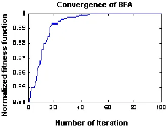
in that generation, before sorting is carried out for reproduction. In this paper, instead of the average value, the minimum value of all the chemotactic cost functions is retained for deciding the bacterium’s health. This speeds up the convergence, because in the average scheme [6], it may not retain the fittest bacterium for the subsequent generation. On the contrary, in this paper, the global minimum bacteria among all chemotactic stages pass on to the subsequent stage. 2) For swarming, the distances of all the bacteria in a new chemotactic stage is evaluated from the global optimum bacterium until that point and not the distances of each bacterium from the rest of the others, as suggested in [5, 6]. The convergence of normalized fitness function with respect to number of iteration available from four loops is shown in Figure 3. It is to be mentioned that for the analysis of V-dipoles, time taken for 10 bacteria case in 1.7 GHz Celeron processor is only 5–6minutes which is much faster than when average value was taken (about 1 hour).
Figure 3. Convergence rate of modified BFA.
The algorithmic steps are described below:
Step 1—Initialization
The following variables are initialized.
1) Number of bacteria (S) to be used in the search. 2) Number of parameters (p) to be optimized. 3) Swimming length Ns
4) Nc the number of iterations in a chemotactic loop (Nc > Ns).
5) Nrethe number of reproduction.
6) Ned the number of elimination and dispersal events.
8) Location of each bacteriumP(p, S,1), i.e., random numbers on [0– 1].
9) dattract,ωattract,hrepelent, and ωrepelent are given of fixed values
Step 2—Iterative algorithm for optimization
This section models the bacterial population chemotaxis, swarming, reproduction, and elimination and dispersal (initially, j =
k = l = 0). For the algorithm updating, θi automatically results in updating of “P”.
1) Elimination-dispersal loop: l=l+ 1 2) Reproduction loop: k=k+ 1 3) Chemotaxis loop: j=j+ 1
These steps have been applied as given in [6].
a) For i = 1, 2, . . ., S, calculate cost function value for each bacteriumias follows.
• Compute value of cost function J(i, j, k, l).
Let Jsw(i, j, k, l) =J(i, j, k, l) +Jcc(θi(j, k, l), P(j, k, l)) P(j, k, l) is the location of bacterium corresponding to the global minimum cost function out of all the generations and chemotactic loops until that point (i.e., add on the cell-to-cell attractant effect for swarming behavior).
• Let Jlast =Jsw(i, j, k, l) to save this value since we may find
a better cost via a run. • End of For loop
b) Fori= 1, 2, . . .,S, take the tumbling/swimming decision • Tumble: Generate a random vector ∆(i) ∈ RP with each
element number
∆m(i) [where m= 1, 2,. . . ,p,] a random number on [0, 1].
• Move: let
θi(j+ 1, k, l) =θi(j, k, l) +C(i) ∆(i) ∆T(i)∆(i)
Fixed step size in the direction of tumble for bacterium i is considered.
• Compute J(i, j+ 1, k, l) and then let
Jsw(i, j+1, k, l) =J(i, j+1, k, l)+Jcc(θi(j+1, k, l), P(j+1, k, l))
• Swim:
(i) letm= 0; (counter for swim length)
• let m=m+ 1
• ifJsw(i, j+ 1, k, l)< Jlast (if doing better)
then let Jlast=Jsw(i, j+ 1, k, l) and
θi(j+ 1, k, l) =θi(j, k, l) +C(i) ∆(i) ∆T(i)∆(i)
use thisθi(j+ 1, k, l) to compute new J(i, j+ 1, k, l) • else, letm=Ns. This is the end of while statement.
c) Go to next bacterium (i+ 1) if i= S (i.e., go to “b”) to process the next bacterium.
4) If j > Nc, go to step 3. In this case, continue chemotaxis since the
life of the bacteria is not over. 5) Reproduction
a) For the given k and l, and for each i = 1, 2, . . . , S, let
Jhealthi = min
j∈{1...Nc}
{Jsw(i, j, k, l)}be the health of the bacterium i. Sort bacteria in order of ascending cost Jhealth (higher cost
means lower health).
b) The Sr = S/2 bacteria with highest Jhealth values die and other Sr bacteria with best value split (and the copies that are made
are placed at the same location as their parent)
6 ) If k < Nre, go to 2; in this case, we have not reached the number
of specified reproduction steps, so we start the next generation in the chemotactic loop.
7) Elimination-dispersal: For i = 1, 2, . . ., S, with probability Ped,
eliminates and disperses each bacterium (this keeps the number of bacteria in the population constant). To do this, if one eliminates a bacterium, simply disperse it to a random location on the optimization domain.
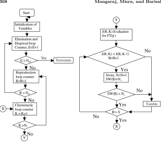
The flow chart of the improved algorithm is shown in Figure 4.
5. SIMULATION
The minimum value of DR is 1.76dB for elementary dipole and maximum value may be infinite for any ideal directive structure.
So range of directivity is kept as
1.76≤DR(ψ)≤ ∞ (22)
J(B, K) < J(B, K-1) B=B+1 E > Ned
J(B, K) Evaluation for FT(y) Initialization of
Variables
Elimination and Dispersal loop Counter, E=E+1
Reproduction loop counter R=R+1
Chemotactic loop counter K = K+1
SW(B) < Ns
X
Y
Swim, N=N+1 SW(B)=Ns
R > Nre
K >Nc
Y
X
B > S Yes
No
No
No
No
No
No
Yes
Yes Yes
Start
Terminate
Tumble
Figure 4. Flowchart of the bacteria foraging algorithm.
So range of Fitness function is defined as
1> F T(ψ)≥0 (23)
So, the intention of our program is to find the minimum value for the fitness function (near to zero) i.e., the place where maximum number of bacteria is found.
Considering Bacteria Foraging Algorithm a MATLAB program has been formulated for V and dipole antennae structure. The foragers find a best included angle i.e.,ψ, which ultimately provides the highest directivity for a particular length of V-dipole depending on our fitness function.
For all the different lengths of V-dipole the parameters for simulations are as follow:
Sb= Number of bacteria = 10
N k= Number of chemotactic steps = 30
N s= Number of swim = 4
N rd= Number of dispersal and elimination = 2
P ed= elimination-dispersal with probability = 0.25
C(i) = the size of the step(variable for all bacteria) taken in the random direction specified by the tumble.
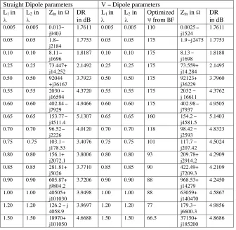
Table 1. Comparative chart for straight and V-dipole antennas.
Straight Dipole parameters V − Dipole parameters L1 in L2 in Zin in DR
in dB
L1 in L2 in Optimized
from BF
Zin in DR
in dB
0.005 0.005 0.013− j9403
1.7611 0.005 0.005 110 0.0025 j1524
1.7611
0.05 0.05 1.8− j2184
1.7753 0.05 0.05 175 1.9 j2475 1.7753
0.10 0.10 8.11 j1696
1.8187 0.10 0.10 175 8.13 j1698
1.8188
0.25 0.25 73.447+ j14.252
2.1492 0.25 0.25 175 73.559+ j14.284
2.1495
0.50 0.50 92044 +j36167
3.7923 0.50 0.50 175 92123+ j36229
3.7960
0.55 0.55 2030 − j16594
4.3720 0.55 0.55 175 2032 j 16611
4.3762
0.60 0.60 402.84 j7929
4.9466 0.60 0.60 175 402.98 j7937
4.9505
0.65 0.65 153.77 j4511.4
5.1307 0.65 0.65 160 154.2 j4581.5
5.1403
0.70 0.70 96.52 j2226
4.0120 0.70 0.70 118 98.42 j2593
4.8323
0.75 0.75 103.1 j178.53
3.4076 0.75 0.75 101 117.7 j207.42
4.5024
0.80 0.80 156.1+ j2072.1
3.8006 0.80 0.80 93 209.78+ j2914.2
4.2909
0.85 0.85 281.81+ j5026
3.7710 0.85 0.85 90 422.49+ j7209.3
4.2109
0.90 0.90 605.87+ j9804.2
3.7206 0.90 0.90 88 968.53+ j14279
4.2450
1.00 1.00 40505+ j101030
3.9498 1.00 1.00 88 63059+
j140470
4.5867
1.20 1.20 126.2 j 4058.9
3.9697 1.20 1.20 77 179.3 j6600.3
4.9856
1.50 1.50 18970+ j101050
4.6688 1.50 1.50 66.5 37150+ j185200 4.8686 λ λ Ω λ λ ψ Ω − − − − − − − − − − − − − − − 6. RESULTS
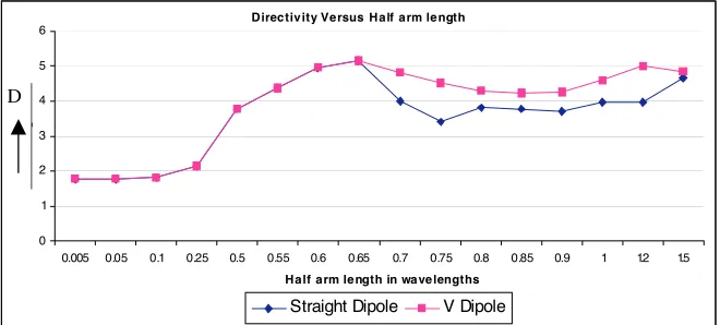
Directiv ity Versus Half arm le ngth
0 1 2 3 4 5 6
0.005 0.05 0.1 0.25 0.5 0.55 0.6 0.65 0.7 0.75 0.8 0.85 0.9 1 1.2 1.5 Half arm le ngth in wa ve lengths
Straight Dipole V Dipole
D
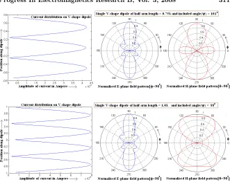
Figure 6. Radiation field patterns for V-antenna for different arm length.
Table 2. % of increase in directivity of V dipole in comparison to
similar length straight dipole.
Length
in 0.005 0.05 0.1 0.25 0.5 0.55 0.7 0.75 0.8 0.85 0.9 1 1.2 1.5 Increase
in DR in %
0.00 0.00 0.01 0.01 0.10 0.10 0.08 0.19 20.45 32.13 12.90 11.67 14.09 16.12 25.594.28
λ 0.6 0.65
7. CONCLUSION
The focus of this paper is to describe the application of the BFA in antenna problem. It is clear from the result that to get good directivity, the length must be selected judiciously. The Method of Moments analysis of this paper would be very helpful to the researcher. Using BFA, this paper establishes a very old concept of providing higher directivity of long-V antenna compared to simple straight dipole. Moreover, some comparative results between symmetrical straight dipole and symmetrical V-dipole with some optimizedψhave been provided using bacteria foraging optimization technique. Similar attempt can also be made for asymmetrical cases using the same programs. Again, the modification made for the BFA can show the faster convergence. This may be applied to any complicated antenna structure including array antenna where time complexity would be of major concern.
REFERENCES
1. Harrington, R. F., Field Computation by Moment Methods, Macmillan, New York, 1968.
2. Thiele, G. A., “Calculation of the current distribution on a thin linear antenna,” IEEE Trans. Antennas Propagat., Vol. AP-14, No. 5, 648–649, September 1966.
3. Balanis, C. A., Antenna Theory: Analysis and Design, 2nd edition, John Wiley & Sons, 1997.
4. Passino, K. M., “Biomimicry of bacterial foraging for distributed optimization and control,” IEEE Control Systems Magazine, Vol. 22, No. 3, 52–67, June 2002.
5. Tripathy, M. and S. Mishra “ Bacteria foraging-based solution to optimize both real power loss and voltage stability limit,” IEEE Transactions on Power Systems, Vol. 22, No. 1, February 2007. 6. Mishra, S., “A hybrid least square-fuzzy bacteria foraging strategy
for harmonic estimation,” IEEE Trans. Evol. Comput., Vol. 9, No. 1, 61–73, Feb. 2005.
7. Tong, M. S., “A stable integral equation solver for electromagnetic scattering by large scatterers with concave surface,” Progress In Electromagnetics Research, PIER 74, 113–130, 2007.
8. Segall, J., S. Block, and H. Berg, “Temporal comparisons in bacterial chemotaxis,” Proc. Nat. Acad. Sci., Vol. 83, 8987–8991, Dec. 1986.
bundles in swimming bacteria,” Nature, Vol. 325, 637–640, Oct. 1987.
10. Losick, R. and D. Kaiser, “Why and how bacteria communicate,”
Sci. Amer., Vol. 276, No. 2, 68–73, 1997.
11. Budrene, E. and H. Berg, “Dynamics of formation of symmetrical patterns by chemotactic bacteria,”Nature, Vol. 376, 49–53, 1995. 12. Misra, I. S., R. S. Chakraborty, and B. B. Mangaraj, “Design, analysis and optimization of V-dipole and its three-element Yagi-Uda array,”Progress In Electromagnetic Research, PIER 66, 137– 156, USA, 2006.
13. Mahanti, G. K., A. Chakrabarty, and S. Das, “Phase-only and amplitude-phase only synthesis of dual-beam pattern linear antenna arrays using floating-point genetic algorithms,”Progress In Electromagnetics Research, PIER 68, 247–259, 2007.
14. Riabi, M. L., R. Thabet, and M. Belmeguenai, “Rigorous design and efficient optimizattion of quarter-wave transformers in metallic circular waveguides using the mode-matching method and the genetic algorithm,” Progress In Electromagnetics Research, PIER 68, 15–33, 2007.
15. Hosseini, S. A. and Z. Atlasbaf, “Optimization of side lobe level and fixing quasi-nulls in both of the sum and difference patterns by using continuous ant colony optimization (ACO) method,”
Progress In Electromagnetics Research, PIER 79, 321–337, 2008. 16. Mahmoud, K. R., M. El-Adawy, S. M. M. Ibrahem, R. Bansal, and
S. H. Zainud-Deen, “A comparison between circular and hexagonal array geometries for smart antenna systems using particle swarm optimization algorithm,” Progress In Electromagnetics Research, PIER 72, 75–90, 2007.
17. Lee, K. C. and J. Y. Jhang, “Application of particle swarm algorithm to the optimization of unequally spaced antenna arrays,” Journal of Electromagnetic Waves and Applications, Vol. 20, 2001–2012, 2006.
18. Guney, K. and M. Onay, “Amplitude-only pattern nulling of linear antenna arrays with the use of Bees algorithm,” Progress In Electromagnetics Research, PIER 70, 21–36, 2007.
19. Hosseini, S. A. and Z. Atlasbaf, “Optimization of side lobe level and fixing quasi-nulls in both of the sum and difference patterns by using continuous ant colony optimization (ACO) method,”
Progress In Electromagnetics Research, PIER 79, 321–337, 2008. 20. Akdagli, A. and K. Guney, “Shaped-beam pattern synthesis
a modified tabu search algorithm,” Microwave and Optical Technology Letters, Vol. 36, 16–20, 2003.
21. Mahmoud, K. R., M. El-Adawy, S. M. M. Ibrahem, R. Bansal, and S. H. Zainud-Deen, “A comparison between circular and hexagonal array geometries for smart antenna systems using particle swarm optimization algorithm,” Progress In Electromagnetics Research, PIER 72, 75–90, 2007.
22. Ayestaran, R. G., J. Laviada, and F. Las-Heras, “Synthesis of passive-dipole arrays with a genetic-neural hybrid method,”
Journal of Electromagnetic Waves and Applications, Vol. 20, 2123–2135, 2006.
23. Lee, Z. J. and C. Y. Lee, “A hybrid search algorithm with heuristics for resource allocation problem,”Information Sciences, Vol. 173, No. 1–3, 155–167, 2005.
24. Juang, C. F., “A hybrid of genetic algorithm and particle swarm optimization for recurrent network design,”IEEE Transactions on Systems Man and Cybernetics - Part B, Vol. 34, 997–1006, 2004. 25. Xu, Z., H. Li, Q. Z. Liu, and J. Y. Li, “Pattern synthesis
of conformal antenna array by the hybrid genetic algorithm,”
Progress In Electromagnetics Research, PIER 79, 75–90, 2008. 26. Mishra, S., “Hybrid least-square adaptive bacterial foraging
strategy for harmonic estimation,” IEE Proc. - Generation Transmission and Distribution, Vol. 152, 379–389, 2005.
27. Passino, K. M., “Biomimicry of bacterial foraging,”IEEE Control Systems Magazine, Vol. 22, 52–67, 2002.
28. Lin, W. and P. X. Liu, “Hammerstein model identification based on bacterial foraging,” Electronics Letters, Vol. 42, 1332–1334, 2006.
29. Kim, D. H., A. Abraham, and J. H. Cho, “A hybrid genetic algorithm and bacterial foraging approach for global optimization,”Information Sciences, Vol. 177, 3918–3937, 2007. 30. Niu, B., Y. Zhu, X. He, and X. Zeng, “Optimum design of PID
controllers using only a germ of intelligence,”6th World Congress on Intelligent Control and Automation, 3584–3588, Dalian, China, June 2006.