Volume 2011, Article ID 490289,10pages doi:10.1155/2011/490289
Research Article
Computationally Efficient DOA and Polarization
Estimation of Coherent Sources with
Linear Electromagnetic Vector-Sensor Array
Zhaoting Liu,
1Jing He,
2and Zhong Liu
11Department of Electronic Engineering, Nanjing University of Science and Technology, Nanjing, Jiangsu 210094, China 2Department of Electrical and Computer Engineering, Concordia University, Montreal, QC, Canada H3G 2W1
Correspondence should be addressed to Zhaoting Liu,[email protected]
Received 3 September 2010; Revised 10 December 2010; Accepted 16 January 2011
Academic Editor: Ana P´erez-Neira
Copyright © 2011 Zhaoting Liu et al. This is an open access article distributed under the Creative Commons Attribution License, which permits unrestricted use, distribution, and reproduction in any medium, provided the original work is properly cited.
This paper studies the problem of direction finding and polarization estimation of coherent sources using a uniform linear electromagnetic vector-sensor (EmVS) array. A novel preprocessing algorithm based on EmVS subarray averaging (EVSA) is firstly proposed to decorrelate sources’ coherency. Then, the proposed EVSA algorithm is combined with the propagator method (PM) to estimate the EmVS steering vector, and thus estimate the direction-of-arrival (DOA) and the polarization parameters by a vector cross-product operation. Compared with the existing estimate methods, the proposed EVSA-PM enables decorrelation of more coherent signals, joint estimation of the DOA and polarization of coherent sources with a lower computational complexity, and requires no limitation of the intervector sensor spacing within a half-wavelength to guarantee unique and unambiguous angle estimates. Also, the EVSA-PM can estimate these parameters by parameter-space searching techniques. Monte-Carlo simulations are presented to verify the efficacy of the proposed algorithm.
1. Introduction
A typical electromagnetic vector-sensor (EmVS) consists of six component sensors configured by two orthogonal triads of dipole and loop antennas with the same phase center. Therefore, an EmVS can simultaneously measure the three components of the electric field and the three components of the magnetic field. Since its introduction into signal processing community [1, 2], a significant number of research has been done on EmVS array processing [3–19]. For application considerations, different types of EmVS containing part of the six sensors are devised and manufactured [3,20,21].
In the study of direction finding applications, conven-tional eigenstructure-based source localization techniques have been extended to the case of the EmVS array. ESPRIT/ MUSIC algorithms using EmVS arrays obtain thorough
investigations [10–12, 16–19]. The signal subspace and noise subspace are usually constructed by decomposing the column space of the data correlation matrix with the eigen-decomposition (or singular value decomposition) techniques [22, 23]. Because the decomposing process is computationally intensive and time consuming, the eigen-structure-based techniques may be unsuitable for many practical situations, especially when the number of vector sensors is large and/or the directions of impinging sources should be tracked in an online manner.
To deal with the coherent signals using the EmVS array, a polarization smoothing algorithm (PSA) has been proposed to restore the rank of signal subspace [19]. The PSA does not reduce the effective array aperture length and has no limit to array geometries. However, the PSA-based method has non-negligible drawbacks. (1) It assumes the intervector sensor spacing within a half-wavelength to guarantee unique and unambiguous angle estimates; (2) it is not able to estimate the polarization of impinging electromagnetic waves; (3) the EmVS type limits the maximum number of resolvable coherent signals.
In this paper, we employ a uniform linear EmVS array to perform parameter estimation of coherent sources. Firstly, to decorrelate the coherent sources, an EmVS sub-array averaging-based pre-processing (EVSA) algorithm is developed. Then the EVSA algorithm is coupled with the propagator method (PM) [24, 25] to estimate parameters of the coherent sources without eigen-decomposition or singular value decomposition unlike the ESPRIT/MUSIC-based methods. By using the vector cross-product of the electric field vector estimate and the magnetic field vector estimate, the proposed EVSA-PM can estimate both the DOA and polarization parameters, hence, can overcome the drawbacks of the PSA-based algorithms to some extent. The vector cross-product estimator is valid to a six-component EmVS array. For the array comprising any types of EmVSs, the EVSA-PM with parameter-space searching techniques is developed to estimate the parameters. The EVSA-PM can be regarded as an extension of the subspace-based method without eigendecomposition (SUMWE) [26] to the case of the EmVS arrays. The SUMWE is also a PM-based method, which estimates the DOA of coherent sources using unpolarized scalar sensors by an iterative angle searching. However, the proposed methods make use of more available electromagnetic information, and hence, should outperform the SUMWE algorithm in accuracy and resolution of DOA estimation.
The rest of this paper is organized as follows. Section 2
formulates the mathematical data model of EmVS array.
Section 3 develops the proposed EmVS-PM. Section 4
presents the simulation results to verify the efficacy of the EmVS-PM.Section 5concludes the paper.
2. Mathematical Data Model
Assume thatK narrowband completely polarized coherent signals impinge upon a uniform linear EmVS array withM
vector sensors (M > 2K), and the array is neither mutual coupling nor cross-polarization effects. The K is known in advance and the kth incident source is parameterized {θk,ϕk,γk,ηk}, where 0≤θk≤π/2 denotes thekth source’s
elevation angle measured from the verticalz-axis, 0≤ϕk ≤
2πrepresents thekth source’s azimuth angle, 0≤γk ≤π/2
refers to the kth source’s auxiliary polarization angle, and −π≤ηk ≤πsymbolizes thekth source’s polarization phase
difference. For a six-component EmVS, the steering vector of
thekth unit-power electromagnetic source signal produces the following 6×1 vector:
cθk,ϕk,γk,ηk
def = ⎡ ⎢ ⎢ ⎢ ⎢ ⎢ ⎢ ⎢ ⎢ ⎢ ⎢ ⎢ ⎢ ⎣
c1,k
c2,k
c3,k
c4,k
c5,k
c6,k
⎤ ⎥ ⎥ ⎥ ⎥ ⎥ ⎥ ⎥ ⎥ ⎥ ⎥ ⎥ ⎥ ⎦ def = ⎡ ⎢ ⎢ ⎢ ⎢ ⎢ ⎢ ⎢ ⎢ ⎢ ⎢ ⎢ ⎢ ⎣
ex,k
ey,k
ez,k
hx,k
hy,k
hz,k
⎤ ⎥ ⎥ ⎥ ⎥ ⎥ ⎥ ⎥ ⎥ ⎥ ⎥ ⎥ ⎥ ⎦ = ⎡ ⎢ ⎢ ⎢ ⎢ ⎢ ⎢ ⎢ ⎢ ⎢ ⎢ ⎢ ⎢ ⎣
cosϕkcosθk −sinϕk
sinϕkcosθk cosϕk
−sinθk 0
−sinϕk −cosϕkcosθk
cosϕk −sinϕkcosθk
0 sinθk
⎤ ⎥ ⎥ ⎥ ⎥ ⎥ ⎥ ⎥ ⎥ ⎥ ⎥ ⎥ ⎥ ⎦ def =Θ(θk,φk)
⎡
⎣sinγkejηk
cosγk
⎤ ⎦
def =g(γk,ηk)
, (1)
where ek def= [ex,k,ey,k,ez,k]T and hk def= [hx,k,hy,k,hz,k]T
denote the electric field vector and the magnetic field vector, respectively.
The intersensor spatial phase factor for the kth inci-dent signal and the mth vector sensor is qm(θk,ϕk) def=
ej2π(xmuk+ymvk)/λ, where u
k def= sinθkcosϕk and vk def=
sinθksinϕk signify the direction cosines along the x-axis
and y-axis, respectively. (xm,ym) is the location of themth
vector sensor,λequals the signals’ wavelength. Denoting the spacing between adjacent vector sensors as (Δx,Δy), we have
xm = x1+ (m−1)Δx, ym = y1+ (m−1)Δy. The 6×1
measurement vector corresponding to themth vector sensor can be expressed as
xm(t)def=xm,1(t),. . .,xm,6(t)
T
=K
k=1
qm
θk,ϕk
cθk,ϕk,γk,ηk
sk(t) +wm(t),
(2)
wherewm(t) = [wm,1(t),. . .,wm,6(t)]T is the additive
zero-mean complex noise and independent to all signals.xm,n(t)
and wm,n(t) refer to the measurement and the noise
corre-sponding to themth vector sensor’snth component, respec-tively; sk(t) represents the kth source’s complex envelope.
Without loss of generality, we consider the signals{sk(t)}are
all coherent so that they are all some complex multiples of a common signals1(t). Then, under the flat-fading multipath
propagation, they can be expressed assk(t)=βks1(t) [26,27],
where βk is the multipath coefficient that represents the
For the entire vector-sensor array, the array manifold,
a(θk,ϕk,γk,ηk)∈C6M×1, is given by
aθk,ϕk,γk,ηk
def
=qθk,ϕk
⊗cθk,ϕk,γk,ηk
, (3)
where ⊗ symbolizes the Kronecker product operator,
q(θk,ϕk) def= [q1(θk,ϕk),. . .,qM(θk,ϕk)]T. With a total ofK
signals, the entire 6M×1 output vector measured by the EmVS array at timethas the complex envelope represented as
z(t)=xT1(t),. . .,xTM(t)
T
=K
k=1
aθk,ϕk,γk,ηk
sk(t) +n(t)
=As(t) +n(t),
(4)
whereA ∈ C6M×K,s(t) ∈ CK×1,n(t) ∈ C6M×1, andA =
[a(θ1,ϕ1,γ1,η1),. . .,a(θK,ϕK,γK,ηK)]; s(t) = [s1(t),. . .,
sK(t)]T,n(t)=[wT1(t),. . .,wMT(t)]T.
3. Algorithm Development
This section is devoted to the algorithm development.
Section 3.1 develops the EVSA algorithm, Section 3.2
describes EVSA-PM algorithm for estimating both DOA and polarization parameters from the available EmVS steering vector estimates andSection 3.3is for parameters estimation by parameter-space searching techniques.
3.1. EVSA Algorithm. Let us consider the subarray averaging scheme with a linear EmVS array, which is divided into
Loverlapping subarrays with K vector sensors and thelth subarray comprises the lth to (l+K −1)th vector sensor, where L = M−K + 1. We use the first vector sensor as a reference (x1 = 0, y1 = 0), and then the corresponding
6K × 1 signal vector is given as
zl(t)def=
xT
l (t),. . .,xTl+K−1(t)
T
=A0Dl−1s(t) +nl(t), (5)
where D ∈ CK×K, and D def= diag(ej2π(Δxu1+Δyv1)/λ,. . .,
ej2π(ΔxuK+ΔyvK)/λ);A
0∈C6K×Kcontains the first 6Krows ofA; nl(t)def= [wTl(t),. . .,wlT+K−1(t)]T. We can calculate the
cross-correlation vectorϕl,n∈C6K×1betweenz
l(t) andxM,n(t) ϕl,n
def=
Ezl(t)xM∗,n(t)
=A0Dl−1E
s(t)sH(t)a∗
M,n+E
nl(t)wM∗,n
=ρM,nrsA0Dl−1β, l=1, . . ., L−1; n=1, . . ., 6,
(6)
where E{·} denotes the expectation, rs def= E{s1(t)s∗1(t)},
ρl,n def= βHa∗l,n, al,n def= [ql(θ1,ϕ1)cn,1,. . .,ql(θK,ϕK)cn,K]T,
β def
= [β1,. . .,βK]T. Similarly, the cross-correlation vector
ϕl,n∈C6K×1betweenzl(t) andx1,n(t) is as follows
ϕl,n def
=Ezl(t)x∗1,n(t)
=ρ1,nrsA0Dl−1β, l=2,. . .,L; n=1,. . ., 6. (7)
Let us rewrite the vectorϕl,nas a 6×Kmatrix
Φl,ndef=
J1ϕl,n,. . .,JKϕl,n
=ρM,nrs
A1Dl−1β,. . .,AKDl−1β
=ρM,nrsAl
β,. . .,DK−1β
=ρM,nrsAlBQT,
(8)
where Jk def= [06,6(k−1),I6,06,6(K−k)]; B def= diag(β1,. . .,βK);
Al is the 6 × K matrix with the column ckql(θk,ϕk),
k = 1,. . ., 6; Q is the K ×K matrix with the column [q1(θk,ϕk),. . .,qK(θk,ϕk)]T. Similarly, the vectorϕl,ncan be
rewritten as
Φl,ndef=
J1ϕl,n,. . .,JKϕl,n
=ρ1,nrsAlBQT. (9)
Therefore, concatenatingΦl,nforl=1,. . .,L−1 andΦl,nfor
l=2,. . ., L, respectively, we can get two correlation matrices
Rndef=
ΦT
1,n,ΦT2,n,. . .,ΦT(L−1),n
T
=ρM,nrsABQ T,
Rndef=
ΦT2,n,Φ
T 3,n,. . .,Φ
T L,n
T
=ρ1,nrsABDQ T,
(10)
whereRn ∈ C6(L−1)×K,Rn ∈C6(L−1)×K, andA def= [AT1,. . .,
AT
L−1]T includes the first 6(L−1) rows ofA. With (10), the
EmVS subarray averaging (EVSA) matrix can be formulated as
Rdef=R1,. . .,R6,R1,. . .,R6
=AΩ, (11)
whereΩdef= rsB[ρM,1QT,. . .,ρM,6QT,ρ1,1DQT,. . .,ρ1,6DQT].
Note that B and D are diagonal matrices with nonzero diagonal elements, and Q is full rank when all sources impinge with the distinct incident directions. Then theRn
andRnare of rankK, and hence,Ris of rankK and can be
used to estimate the DOA and the polarization parameters of the coherent sources.
In realistic cases where only a finite number of snapshots are available, the cross-correlation vectorϕl,n and ϕl,n can
be estimated as ϕl,n =
S
t=1zl(t)xM∗,n(t)/S and ϕl,n =
S
t=1zl(t)x∗1,n(t)/S, whereSdenotes the number of snapshots.
Withϕl,nandϕl,n, the matrixRis accordingly obtained using
(8)–(11).
signals are coherent and the others are uncorrelated with these signals and with each other. Then after some algebraic manipulations, we can obtain
Rn=ρM,nrs1ABQ T+ARA HM,nQT,
Rn=ρ1,nrs1ABDQ
T+AD RA H 1,nQT,
(12)
where ρl,n def= β H
a∗l,n, β def= [β1,. . .,βK1, 0,. . ., 0]
T, B def
= diag(β1,. . .,βK1, 0,. . ., 0),rsk
def
= E{sk(t)s∗k(t)},R
def
= diag(0,
. . .,rsK1 +1,. . .,rsK), Al,n def
= diag(ql(θ1,ϕ1)cn,1,. . .,ql(θK,
ϕK)cn,K). It is easy to find that the rank ofRn and Rn still
equalsKwhen all sources impinge with the distinct incident directions.
Remarks. (1) The proposed EVSA algorithm is still effective in the case of partly coherent or incoherent sources in which there exist two incoherent sources with the same incident directions but with the distinct polarizations. As shown in the appendix, the matrixRdefined in (11) has full rank. However, neither the PSA [19] nor the SUMWE [26] algorithm can be so.
(2) The EVSA algorithm needs low computations. As seen from (6) and (7), the EVSA only needs compute the cross-correlations, which require 72(L−1) cross-correlation operations. However, most of EmVS direction finding algo-rithms require to compute the correlations of all array data with (6M)2correlation operations.
(3) The EVSA-based method may estimate both DOA and polarization parameters, while the PSA-based one can only estimate the DOA parameters because of the polariza-tion smoothing.
(4) From (11), the EVSA algorithm can decorrelate more coherent sources than the PSA can do. The EVSA algorithm can decorrelate up-to L − 2 coherent sources regardless of EmVS’s types, while the PSA can only decorrelate 6 coherent sources for six-component EmVS array, 4 for quadrature polarized array [19] and 2 for dual polarized array [19]. By coupling the forward/backward (FB) averaging technique [27], the maximum number of the coherent signals decorrelated by the PSA is doubled, however, it is only valid for the case of the symmetric array, for instance, uniform linear array, to which the proposed method is limited.
3.2. EVSA-PM Algorithm for Estimating Parameters from the
EmVS Steering Vector. The EVSA-PM algorithm performs
the estimation of the coherent sources’ DOA and polariza-tion parameters by using the vector cross-product operapolariza-tion of the estimated electric field vector and magnetic field vector. For this purpose, we define an exchange matrix
E=e1,e7,. . .,e6(L−2)+1,e2,e8,. . .,e6(L−2)+2,. . ., e6,e12,. . .,e6(L−1)
, (13)
whereei is the 6(L−1) dimensional unit vector whose ith
element is 1 and other elements are zero. In addition, we define
Redef=ETR=AeΩ, (14)
Aedef= ETA=
ATe,1,. . .,ATe,6
T
, (15)
where Ae ∈ C6(L−1)×K, Ae,n ∈ C(L−1)×K(n = 1, . . ., 6)
is a submatrix whosekth column is given as qe(θk,ϕk)cn,k
with qe(θk,ϕk) def= [q1(θk,ϕk),. . .,qL−1(θk,ϕk)]T. These
submatrices are related with each other by
Ae,n=Ae,1Λn, (16)
whereΛn∈CK×KandΛndef=diag(dn,1,. . .,dn,K) withdn,kdef=
cn,k/c1,k denoting thekth source’s invariant factor between
the first and thenth EmVS component. We can divideAe,ninto
Ae,n=
⎡ ⎣A
(1) e,n
A(2)e,n
⎤
⎦, n = 1,. . ., 6, (17)
whereA(1)e,n ∈CK×K andA(2)e,n ∈C(L−1−K)×K. Therefore,Ae,n
can be rewritten as
Ae=
⎡ ⎣A(1)e,1
U
⎤
⎦, (18)
whereU def= [(A(2)e,1)T, (A (1) e,2)T, (A
(2)
e,2)T,. . ., (A (1) e,6)T, (A
(2) e,6)T]T.
Obviously,A(1)e,nis a matrix with full rank. TheK×(6L−6−
K) propagator matrixP can be defined as a unique linear operator which relates the matricesA(1)e,1 andUthrough the
equation
PHA(1)
e,1=U. (19)
We partitionPH intoPH = [PT
1,PT2,. . .,PT11]T, whereP1to P11have the dimensions identical toA(2)e,1,A(1)e,2,A(2)e,2,A(1)e,3,A(2)e,3, A(1)e,4,A
(2) e,4,A
(1) e,5,A
(2) e,5,A
(1) e,6, andA
(2)
e,6, respectively. Thus, we have
P1A(1)e,1=A (2)
e,1, (20)
P2n−1A(1)e,1=Ae,1(2)Λn, n=2,. . ., 6. (21)
Equations (20) and (21) together yield
P†1P2n−1=A(1)e,1Λn
A(1)e,1
−1
, n=2,. . ., 6, (22)
where†denotes the Pseudo inverse.
Equation (22) suggests that the matricesP†1P2n−1 (n =
−10 0 10 20 30 40 10−3
10−2 10−1 100 101 102
SNR (dB)
D
O
AR
M
S
E(
d
eg
)
0.5λ 2λ
4λ 8λ
(a)
−10 0 10 20 30 40
10−3 10−2 10−1 100 101 102
SNR (dB)
D
O
A
R
MSE
(deg)
0.5λ 2λ
4λ 8λ
(b)
Figure1: DOA estimates RMSE of the proposed EVSA-PM against SNRs. (a) Source 1, (b) source 2.
matching the eigenvectors of the different matricesP†1P2n−1
(n = 2,. . ., 6) [11]. With the estimated c(θk,ϕk,γk,ηk) =
[1,d2,k,. . .,d6,k]T, the Poynting vector estimates can be
obtained by the vector cross-product operation and then the DOA and polarization parameters are estimated from the normalized Poynting vectors [11]. For a dipole triad array or loop triad array, the estimates of the electric field vectorekor
the magnetic field vectorhkcan be done in the same way. In
this case, the DOA and polarization parameter estimates can be obtained using the amplitude-normalized estimates of the electric or magnetic field steering vector [3].
In order to calculate the propagator matrixP, we divide the matrix Re into Re = [RTe1,RTe2]T, where Re1 and Re2
consist of the firstK rows and the last 6L−6−K rows of
Re. In the noise-free case, we havePHRe1=Re2. In the noise
case, a least squares solution can be used to estimateP
P=Re1RHe1
−1
Re1RHe2. (23)
3.3. EVSA-PM Algorithm for Estimating Parameters by Angle
Searching. The EVSA-PM is also applied to the uniform
linear array comprising any types of identical EmVSs. In the case, the estimates of DOA and polarization parameters can-not be extracted from the estimates of the steering vectors. However, they are obtainable by the use of parameter-space searching techniques. We here use two-dimensional angle searching to estimate the DOA.
Consider N-component EmVS array (2 ≤ N ≤ 6), then the matrixAe in (15) can be rewritten asAe = [ATe,1,
. . .,ATe,N]T∈CN(L−1)×K, andAe,ncan also be rewritten as Ae,n=Qe
n, n=1,. . .,N, (24)
whereQe def= [qe(θ1,ϕ1),. . .,qe(θK,ϕK)]∈C(L−1)×K,
n def
= diag(cn,1,. . .,cn,K)∈CK×K.
Defining gn def= [0L−1,(L−1)(n−1),IL−1,0L−1,(L−1)(N−n)] ∈
R(L−1)×N(L−1), we have R g def=
N
n=1gnRe = QeΠΩ, where
Π def
= N
n=1Πn. PartitioningRgintoRg =[RTg1RTg2]T, where Rg1 and Rg2 consist of the first K rows and the last L−
1 −K rows of Rg, we have the propagator matrix P =
(Rg1RHg1)
−1
Rg1RHg2. Then the source’s DOA parameters can be
estimated as
θk,ϕk
=arg min
{θ,ϕ}
qHe
θ,ϕΨΨHqe
θ,ϕ, (25)
whereΨdef= [PT,−I
L−1−K]T.
4. Simulations
We conduct computer simulations to evaluate the perfor-mances of the proposed EVSA-PM. Comparison with the PSA based [19] PM (PSA-PM) and the SUMWE algorithm [26] is also made. For proposed EVSA-PM algorithm, the parameter estimates shown in Figures1–5are extracted from the EmVS steering vector, and those shown inFigure 6are obtained by angle searching. The performance metrics used is the root mean square errors (RMSEs) of the sources’ 2-D DOA and the polarization parameters estimates, where the RMSE ofkth source’s 2-D DOA estimate is defined as
RMSEk=
1 2 ⎧ ⎪ ⎨ ⎪ ⎩ $ % % % &1
E
⎛ ⎝E
e=1
θe,k−θk
2
⎞ ⎠
+ $ % % % &1
E
⎛ ⎝E
e=1
ϕe,k−ϕk
2
⎞ ⎠ ⎫ ⎪ ⎬ ⎪ ⎭,
−10 0 10 20 30 40 10−3
10−2 10−1 100 101 102
SNR (dB)
0.5λ 2λ
4λ 8λ 103
P
olar
RMSE
(deg)
(a)
−10 0 10 20 30 40
10−3 10−2 10−1 100 101 102
SNR (dB)
0.5λ 2λ
4λ 8λ
P
olar
RMSE
(deg)
(b)
Figure2: Polarization state estimates RMSE of the proposed EVSA-PM against SNRs. (a) Source 1, (b) source 2.
PSA-PM
SUMWE CRB
−10 0 10 20 30 40
10−3 10−2 10−1 100 101 102
SNR (dB)
D
O
A
R
MSE
(deg)
EVSA-PM (Δ=4λ) EVSA-PM (Δ=λ/2)
(a)
PSA-PM
SUMWE CRB
−10 0 10 20 30 40
10−3 10−2 10−1 100 101 102
SNR (dB)
D
O
A
R
MSE
(deg)
EVSA-PM (Δ=4λ) EVSA-PM (Δ=λ/2)
(b)
Figure3: DOA estimate RMSEs of EVSA-PM, PSA-PM, and SUMWE against SNRs. (a) Source 1, (b) source 2.
and the RMSE ofkth source’s polarization state estimate is defined as
RMSEk=1
2 ⎧ ⎪ ⎨ ⎪ ⎩ $ % % % &1
E
⎛ ⎝E
e=1
γe,k−γk
2
⎞ ⎠
+ $ % % % &1
E
⎛ ⎝E
e=1
ηe,k−ηk
2
⎞ ⎠ ⎫ ⎪ ⎬ ⎪ ⎭,
(27)
where θe,k, ϕe,k, γe,k, and ηe,k symbolize the eth Monte
Carlo trial’s estimates for the kth source’s directions and polarization states andEis the total Monte Carlo trials. In the simulations,E=500.
Figures1and2plot the RMSEs of the sources’ DOA and polarization estimates against signal-to-noise ratio (SNR) levels using the EVSA-PM. The SNR is defined as SNR = (1/K)Kk=1|sk|2/σn2, whereσn2is the noise power lever. Two
equal-power narrowband coherent signals impinge with parametersθ1 =75◦,ϕ1=35◦,γ1 =45◦,η1 = −90◦,θ2 =
80◦,ϕ2 =30◦,γ2 = 45◦, andη2 =90◦, and the multipath
coefficient is set toβ2 = exp(j∗50◦). The uniform linear
array consists of 12 six-component EmVSs. The intervector sensor spacing is set asΔ = .Δ2
x+Δ2y = 0.5λ, 2λ, 4λ, and
EVSA-PM (Δ=4λ) EVSA-PM (Δ=λ/2) PSA-PM
SUMWE CRB
101 102 103
Snapshot number 10−2
10−1 100 101 102
D
O
A
R
MSE
(deg)
(a)
EVSA-PM (Δ=4λ) EVSA-PM (Δ=λ/2) PSA-PM
SUMWE CRB
101 102 103
Snapshot number 10−2
10−1 100 101 102
D
O
A
R
MSE
(deg)
(b)
Figure4: DOA estimate RMSEs of EVSA-PM, PSA-PM and SUMWE against the number of snapshots. (a) Source 1, (b) source 2.
65 66 67 68 69 70 71 72 73 74 75 0
10 20 30 40 50 60 70
Elevation angle
EVSA-PM
(a)
65 66 67 68 69 70 71 72 73 74 75 0
10 20 30 40 50 60
Elevation angle
PSA-PM
(b)
65 66 67 68 69 70 71 72 73 74 75 Elevation angle
SUMWE
0 5 10 15 20 25 30
(c)
contributes to the estimation accuracy enhancement. Since the estimation of DOA and polarization is extracted from the EmVS steering vector, which contains no time-delay phase factor, we can obtain more accurate but unambiguous estimates of coherent source using an aperture extension array without a corresponding increase in hardware and software costs [12].
Figures 3 and 4 make the comparison between the proposed algorithm with PSA-PM and SUMWE under different SNRs and number of snapshots. The impinging signal parameters are same as in Figures 1 and 2. We use 300 snapshots inFigure 3and set SNR=20 dB inFigure 4. For the proposed algorithm, a uniform linear array with 8 dipole-triads, separated byΔ = λ/2 and 4λ is considered. For the PSA-PM, we use an L-shape geometry, with 8 dipole-triads uniformly placed alongx-axis for estimating uk and
8 dipole-triads uniformly placed alongy-axis for estimating
vk. For the SUMWE, we use an L-shape geometry, with
12 unpolarized scalar sensors uniformly placed along x -axis for estimating uk and 12 unpolarized scalar sensors
uniformly placed alongy-axis for estimatingvk. Hence, the
hardware costs of the SUMWE and the presented algorithm are comparable. The intersensor displacement for the PSA-PM and SUMWE is a half-wavelength, since these two algorithms would suffer angle ambiguities when two sensors are spaced over a half-wavelength. The curves in these two figures unanimously demonstrate that the proposed EVSA-PM withΔ=4λcan offer performance superior to those of the PSA-PM and SUMWE.
From the computational complexity analysis, the major computational costs involved in the three algorithms are the calculation of the corresponding propagator and correlation matrix, and the numbers of multiplications required by the EVSA-PM, the PSA-PM, and SUMWE are in the order of
O(3M1KF+ 18(M1−1)F)≈174F,O(2M1KF+ 6M12F)≈
416F, and O(2M2KF + 4(M2−1)F) ≈ 92F, respectively,
where M1 = 8, M2 = 12, and F denotes the number of
snapshots. Therefore, the proposed EVSA-PM also is more computationally efficient than the PSA-PM.
The proposed EVSA-PM can fully exploit polarization diversity to resolve closely spaced sources with distinct polarizations. To verify this performance, we assume two incident coherent sources with parametersθ1 = 70◦,θ2 =
70.5◦,ϕ1 =90◦,ϕ2 =90◦,γ1 =45◦,γ2 =45◦,η1 = −90◦,
andη2 =90◦. Others simulation conditions are the same as
that inFigure 4, except that the SNR is set at 35 dB.Figure 5
shows the histogram of the estimated elevation using the three methods based on 500 independent trials. From the figure, we can observe that the proposed EVSA-PM can resolve the closely spaced sources. However, the other two methods fail.
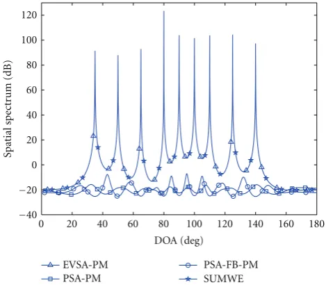
Figure 6plots the spatial spectrum to present comparison of the maximum numbers of coherent signals, which can be, respectively, resolved by the proposed algorithm, the SUMWE, the PSA-PM, and the PSA-FB-PM which combines the PSA with the FB averaging technique [27]. We consider a uniform linear array comprised of 20 unpolarized scalar sensors for the SUMWE and 20 quadrature polarized vector
0 20 40 60 80 100 120 140 160 180 −40
−20 0 20 40 60 80 100 120
DOA (deg)
Spatial
spect
ru
m
(dB)
EVSA-PM PSA-PM
PSA-FB-PM SUMWE
Figure6: Spatial spectrum of EVSA-PM, PSA-PM, PSA-FB-PM, and SUMWE for nine coherent sources.
sensors [19] (i.e., N = 4, M = 20) for all the other three algorithms and estimate the sources’ direction by angle searching. The intervector sensor spacing of array is a half-wavelength. Like [19], we assume zero elevation incident angle (θk =90◦) and randomly chosen polarizations for all
sources, and set SNR=15 dB.
Nine equal power, coherent sources with the azimuth incident angles 35◦, 50◦, 65◦, 80◦, 90◦, 100◦, 110◦, 125◦, and 140◦ are considered, and the corresponding multipath coefficients βk = exp(j ∗10◦(k−1)),k = 1,. . ., 9. This
figure shows that the proposed EVSA-PM and the SUMWE successfully resolve the nine coherent signals, while the PSA-PM, and the PSA-FB-PM fail to do so. This is due to the factor that the PSA-PM and the PSA-FB-PM, respectively, only can resolve min(N,M−1)=4 and min(2N,M−1)=8 coherent sources at most, while the proposed EVSA-PM can resolveL−2 coherent sources (L = M−K + 1), and the maximum number of coherent signals resolved using the SUMWE is equal to that using the EVSA-PM.
5. Conclusions
Appendix
From (12), we can obtain
[R1,. . .,R6]def=AFG , (A.1)
where F def= diag (rs1β1,. . ., rs1βK1, rsK1 +1qM(θK1+1,ϕK1+1),. . ., rsKqM(θK,ϕK))
Gdef= ⎡ ⎢ ⎢ ⎢ ⎢ ⎢ ⎢ ⎢ ⎢ ⎢ ⎢ ⎢ ⎢ ⎢ ⎢ ⎢ ⎢ ⎣
ρM,1hT1 ρM,2hT1 . . . ρM,6hT1
..
. ... . .. ...
ρM,1hTK1 ρM,2h
T
K1 . . . ρM,6h
T K1
c1,K1+1h
T
K1+1 c2,K1+1h
T
K1+1 . . . c6,K1+1h
T K1+1
..
. ... . .. ...
c1,KhTK c2,KhTK . . . c6,KhTK
⎤ ⎥ ⎥ ⎥ ⎥ ⎥ ⎥ ⎥ ⎥ ⎥ ⎥ ⎥ ⎥ ⎥ ⎥ ⎥ ⎥ ⎦
hkdef=
q1θk,ϕk
,. . ., qKθk,ϕk
T
.
,
(A.2)
The matrix A is of full column rank due to the distinct polarizations (although there are two sources from the same direction). The diagonal matrixF has full rank. If the two sources have the same incident directions but with the distinct polarizations, and are uncorrelated with each other (i.e., the two sources are not all included in the set consisting of the firstK1coherent sources), theK×6KmatrixGis of full
row rank. Therefore, in this scenario, the matrix [R1,. . .,R6]
is of rankK. Similarly, the matrix [R1,. . .,R6] also is of rank
K. Thus, the matrixRdefined in (11) still has full rank.
References
[1] A. Nehorai and E. Paldi, “Vector-sensor array processing for electromagnetic source localization,” IEEE Transactions on Signal Processing, vol. 42, no. 2, pp. 376–398, 1994.
[2] J. Li, “Direction and polarization estimation using arrays with small loops and short dipoles,”IEEE Transactions on Antennas and Propagation, vol. 41, no. 3, pp. 379–386, 1993.
[3] K. T. Wong, “Direction finding/polarization estimation— dipole and/or loop triad(s),”IEEE Transactions on Aerospace and Electronic Systems, vol. 37, no. 2, pp. 679–684, 2001. [4] B. Hochwald and A. Nehorai, “Polarimetric modeling and
parameter estimation with applications to remote sensing,” IEEE Transactions on Signal Processing, vol. 43, no. 8, pp. 1923– 1935, 1995.
[5] X. Gong, Z. Liu, Y. Xu, and M. Ishtiaq Ahmad, “Direction-of-arrival estimation via twofold mode-projection,” Signal Processing, vol. 89, no. 5, pp. 831–842, 2009.
[6] J. Tabrikian, R. Shavit, and D. Rahamim, “An efficient vector sensor configuration for source localization,” IEEE Signal Processing Letters, vol. 11, no. 8, pp. 690–693, 2004.
[7] S. Miron, N. Le Bihan, and J. I. Mars, “Quaternion-MUSIC for vector-sensor array processing,”IEEE Transactions on Signal Processing, vol. 54, no. 4, pp. 1218–1229, 2006.
[8] C. C. Ko, J. Zhang, and A. Nehorai, “Separation and tracking of multiple broadband sources with one electromagnetic vector sensor,”IEEE Transactions on Aerospace and Electronic Systems, vol. 38, no. 3, pp. 1109–1116, 2002.
[9] C. Paulus and J. I. Mars, “Vector-sensor array processing for polarization parameters and DOA estimation,”EURASIP Journal on Advances in Signal Processing, vol. 2010, Article ID 850265, 3 pages, 2010.
[10] Y. Xu, Z. Liu, K. T. Wong, and J. Cao, “Virtual-manifold ambi-guity in HOS-based direction-finding with electromagnetic vector-sensors,”IEEE Transactions on Aerospace and Electronic Systems, vol. 44, no. 4, pp. 1291–1308, 2008.
[11] K. T. Wong and M. D. Zoltowski, “Closed-form direction finding and polarization estimation with arbitrarily spaced electromagnetic vector-sensors at unknown locations,”IEEE Transactions on Antennas and Propagation, vol. 48, no. 5, pp. 671–681, 2000.
[12] M. D. Zoltowski and K. T. Wong, “ESPRIT-based 2-D direc-tion finding with a sparse uniform array of electromagnetic vector sensors,”IEEE Transactions on Signal Processing, vol. 48, no. 8, pp. 2195–2204, 2000.
[13] K. T. Wong, “Blind beamforming geolocation for wideband-FFHs with unknown hop-sequences,” IEEE Transactions on Aerospace and Electronic Systems, vol. 37, no. 1, pp. 65–76, 2001.
[14] H. Jiacai, S. Yaowu, and T. Jianwu, “Joint estimation of DOA, frequency, and polarization based on cumulants and UCA,” Journal of Systems Engineering and Electronics, vol. 18, no. 4, pp. 704–709, 2007.
[15] K. C. Ho, K. C. Tan, and A. Nehorai, “Estimating direc-tions of arrival of completely and incompletely polarized signals with electromagnetic vector sensors,”IEEE Transac-tions on Signal Processing, vol. 47, no. 10, pp. 2845–2852, 1999.
[16] K. T. Wong and M. D. Zoltowski, “Uni-vector-sensor ESPRIT for multisource azimuth, elevation, and polarization estima-tion,”IEEE Transactions on Antennas and Propagation, vol. 45, no. 10, pp. 1467–1474, 1997.
[17] K. T. Wong and M. D. Zoltowski, “Self-initiating MUSIC-based direction finding and polarization estimation in spatio-polarizational beamspace,”IEEE Transactions on Antennas and Propagation, vol. 48, no. 8, pp. 1235–1245, 2000.
[18] M. D. Zoltowski and K. T. Wong, “Closed-form eigenstruc-ture-based direction finding using arbitrary but identical subarrays on a sparse uniform Cartesian array grid,” IEEE Transactions on Signal Processing, vol. 48, no. 8, pp. 2205–2210, 2000.
[19] D. Rahamim, J. Tabrikian, and R. Shavit, “Source localization using vector sensor array in a multipath environment,”IEEE Transactions on Signal Processing, vol. 52, no. 11, pp. 3096– 3103, 2004.
[20] Y. Wu, H. C. So, C. Hou, and J. Li, “Passive localization of near-field sources with a polarization sensitive array,”IEEE Transactions on Antennas and Propagation, vol. 55, no. 8, pp. 2402–2408, 2007.
[21] M. Kanda and D. A. Hill, “A three-loop method for deter-mining the radiation characteristics of an electrically small source,”IEEE Transactions on Electromagnetic Compatibility, vol. 34, no. 1, pp. 1–3, 1992.
[22] R. O. Schmidt, “Multiple emitter location and signal param-eter estimation,”IEEE Transactions on Antennas and Propaga-tion, vol. 34, no. 3, pp. 276–280, 1986.
[24] N. Tayem and H. M. Kwon, “L-shape 2-dimensional arrival angle estimation with propagator method,”IEEE Transactions on Antennas and Propagation, vol. 53, no. 5, pp. 1622–1630, 2005.
[25] C. Gu, J. He, X. Zhu, and Z. Liu, “Efficient 2D DOA estimation of coherent signals in spatially correlated noise using electro-magnetic vector sensors,”Multidimensional Systems and Signal Processing, vol. 21, no. 3, pp. 239–254, 2010.
[26] J. Xin and A. Sano, “Computationally efficient subspace-based method for direction-of-arrival estimation without eigendecomposition,”IEEE Transactions on Signal Processing, vol. 52, no. 4, pp. 876–893, 2004.