Volume 2007, Article ID 95281,17pages doi:10.1155/2007/95281
Research Article
Low-Complexity Geometry-Based MIMO Channel Simulation
Florian Kaltenberger,1Thomas Zemen,2and Christoph W. Ueberhuber3 1Austrian Research Centers GmbH (ARC), Donau-City-Strasse 1, 1220 Vienna, Austria 2ftw. Forschungszentrum Telekommunikation Wien, Donau-City-Strasse 1, 1220 Vienna, Austria 3Institute for Analysis and Scientific Computing, Vienna University of Technology,
Wiedner Hauptstrasse 8-10/101, 1040 Vienna, Austria
Received 30 September 2006; Revised 9 February 2007; Accepted 18 May 2007
Recommended by Marc Moonen
The simulation of electromagnetic wave propagation in time-variant wideband multiple-input multiple-output mobile radio channels using a geometry-based channel model (GCM) is computationally expensive. Due to multipath propagation, a large number of complex exponentials must be evaluated and summed up. We present a low-complexity algorithm for the implementa-tion of a GCM on a hardware channel simulator. Our algorithm takes advantage of the limited numerical precision of the channel simulator by using a truncated subspace representation of the channel transfer function based on multidimensional discrete pro-late spheroidal (DPS) sequences. The DPS subspace representation offers two advantages. Firstly, only a small subspace dimension is required to achieve the numerical accuracy of the hardware channel simulator. Secondly, the computational complexity of the subspace representation isindependentof the number of multipath components (MPCs). Moreover, we present an algorithm for the projection of each MPC onto the DPS subspace inO(1) operations. Thus the computational complexity of the DPS subspace algorithm compared to a conventional implementation is reduced by more than one order of magnitude on a hardware channel simulator with 14-bit precision.
Copyright © 2007 Florian Kaltenberger et al. This is an open access article distributed under the Creative Commons Attribution License, which permits unrestricted use, distribution, and reproduction in any medium, provided the original work is properly cited.
1. INTRODUCTION
In mobile radio channels, electromagnetic waves propagate from the transmitter to the receiver via multiple paths. A geometry-based channel model (GCM) assumes that ev-ery multipath component (MPC) can be modeled as a plane wave, mathematically represented by a complex expo-nential function. The computer simulation of time-variant wideband multiple-input multiple-output (MIMO) chan-nels based on a GCM is computationally expensive, since a large number of complex exponential functions must be evaluated and summed up.
This paper presents a novel low-complexity algorithm for the computation of a GCM on hardware channel simulators. Hardware channel simulators [1–5] allow one to simulate mobile radio channels in real time. They consist of a pow-erful baseband signal processing unit and radio frequency frontends for input and output. In the baseband processing unit, two basic operations are performed. Firstly, the channel impulse response is calculated according to the GCM. Sec-ondly, the transmit signal is convolved with the channel
im-pulse response. The processing power of the baseband unit limits the number of MPCs that can be calculated and hence the model accuracy. We note that the accuracy of the channel simulator is limited by the arithmetic precision of the base-band unit as well as the resolution of the analog/digital con-verters. On the ARC SmartSim channel simulator [2], for ex-ample, the baseband processing hardware uses 16-bit fixed-point processors and an analog/digital converter with 14-bit precision. This corresponds to a maximum achievable accu-racy ofEmax=2−13.
inO(1) operations from the MPC parameters given by the model. Furthermore, the subspace representation is indepen-dent of the number of MPCs. Thus, in the hardware sim-ulation of wireless communication channels, the number of paths can be increased and more realistic models can be com-puted. By adjusting the dimension of the subspace, the ap-proximation error can be made smaller than the numerical precision given by the hardware, allowing one to trade accu-racy for efficiency. Using multidimensional DPS sequences, the DPS subspace representation can also be extended to sim-ulate time-variant wideband MIMO channel models.
One particular application of the new algorithm is the simulation of Rayleigh fading processes using Clarke’s [7] channel model. Clarke’s model for time-variant frequency-flat single-input single-output (SISO) channels assumes that the angles of arrival (AoAs) of the MPCs are uniformly distributed. Jakes [8] proposed a simplified version of this model by assuming that the number of MPCs is a multiple of four and that the AoAs are spaced equidistantly. Jakes’ model reduces the computational complexity of Clarke’s model by a factor of four by exploiting the symmetry of the AoA dis-tribution. However, the second-order statistics of Jakes’ sim-plification do not match the ones of Clarke’s model [9] and Jakes’ model is not wide-sense stationary [10]. Attempts to improve the second-order statistics while keeping the re-duced complexity of Jakes’ model are reported in [6,9–14]. However, due to the equidistant spacing of the AoAs, none of these models achieves all the desirable statistical properties of Clarke’s reference model [15]. Our new approach presented in this paper allows us to reduce the complexity of Clarke’s original model by more than an order of magnitude without imposing any restrictions on the AoAs.
Contributions of the paper
(i) We apply the DPS subspace representation to derive a low-complexity algorithm for the computation of the GCM.
(ii) We introduce approximate DPS wave functions to cal-culate the projection onto the subspace inO(1) oper-ations.
(iii) We provide a detailed error and complexity analysis that allows us to trade efficiency for accuracy.
(iv) We extend the DPS subspace projection to multiple di-mensions and describe a novel way to calculate multi-dimensional DPS sequences using the Kronecker prod-uct formalism.
Notation. Let Z, R, and C denote the set of integers, real and complex numbers, respectively. Vectors are denoted by
vand matrices byV. Their elements are denoted byvi and
Vi,l, respectively. Transposition of a vector or a matrix is
in-dicated by ·T and conjugate transposition by ·H. The Eu-clidean (2) norm of the vector ais denoted by a. The Kronecker product and the Khatri-Rao product (columnwise Kronecker product) are denoted by ⊗and , respectively. The inner product of two vectors of lengthN is defined as
x,y =N−1
i=0 xiyi∗, where·∗denotes complex conjugation.
If X is a discrete index set,|X|denotes the number of
el-Scatterer
Scatterer
Transmitter Receiver
v
η1ej2πω1t
η2ej2πω2t η0ej2πω0t
Figure1: GCM for a time-variant frequency-flat SISO channel. Sig-nals sent from the transmitter, moving at speedv, arrive at the re-ceiver via different paths. Each MPCphas complex weightηpand
Doppler shiftωp[16].
ements of X. IfX is a continuous region,|X|denotes the Lebesgue measure ofX. AnN-dimensional sequencevmis a function fromm∈ZNontoC. For anN-dimensional, finite
index setI ⊂ ZN, the elements of the sequencevm,m ∈ I,
may be collected in a vectorv. For a parameterizable func-tion f,{f}denotes the family of functions over the whole parameter space. The absolute value, the phase, the real part, and the imaginary part of a complex variableaare denoted by|a|,Φ(a),a, anda, respectively.E{·}denotes the ex-pectation operator.
Organization of the paper
In Section 2, a subspace representation of time-variant frequency-flat SISO channels based on one-dimensional DPS sequences is derived. The main result of the paper, that is, the low-complexity calculation of the basis coefficients of the DPS subspace representation, is given inSection 3.Section 4
extends the DPS subspace representation to higher dimen-sions, enabling the computer simulation of wideband MIMO channels. A summary and conclusions are given inSection 5.
Appendix Aproposes a novel way to calculate the multidi-mensional DPS sequences utilizing the Kronecker product.
Appendix Bgives a detailed proof of a central theorem. A list of symbols is defined inAppendix C.
2. THE DPS SUBSPACE REPRESENTATION
2.1. Time-variant frequency-flat SISO geometry-based
channel model
We start deriving the DPS subspace representation for the generic GCM for time-variant frequency-flat SISO channels depicted in Figure 1. The GCM assumes that the channel transfer functionh(t) can be written as a superposition of PMPCs:
h(t)=
P−1
p=0
ηpe2π jωpt, (1)
where each MPC is characterized by its complex weightηp,
−νDmax νDmax
−12 12
H(ν)
Figure 2: Doppler spectrum H(ν) of the sampled time-variant
channel transfer functionhm. The maximum normalized Doppler
bandwidth 2νDmax is much smaller than the available normalized channel bandwidth.
Doppler shiftωp. With 1/TSdenoting the sampling rate of
the system, the sampled channel transfer function can be written as
hm=h
mTS
=
P−1
p=0
ηpe2π jνpm, (2)
whereνp=ωpTSis the normalized Doppler shift of thepth
MPC. We refer to (2) as the sum of complex exponentials (SoCE) algorithm for computing the channel transfer func-tionhm.
We assume that the normalized Doppler shifts νp are
bounded by the maximum (one-sided) normalized Doppler bandwidthνDmax, which is given by the maximum speedvmax of the transmitter, the carrier frequency fC, the speed of light
c, and the sampling rate 1/TS,
νp≤νDmax= vmaxfC
c TS. (3)
In typical wireless communication systems, the maximum normalized Doppler bandwidth 2νDmaxis much smaller than the available normalized channel bandwidth (seeFigure 2):
νDmax 1
2. (4)
Thus, the channel transfer function (1) is highly oversam-pled.
Clarke’s model [17] is a special case of (2) and assumes that the AoAsψpof the impinging MPCs are distributed
uni-formly on the interval [−π,π) and thatE{|ηp|2} =1/P. The
normalized Doppler shiftνpof thepth MPC is related to the
AoAψpbyνp=νDmaxcos(ψp). Jakes’ model [8] and its
vari-ants [9–14] assume that the AoAsψpare spaced equidistantly
with some (random) offsetϑ: ψp= 2π p
+ϑ
P , p=0,. . .,P−1. (5) If P is a multiple of four, symmetries can be utilized and only P/4 sinusoids have to be evaluated [8]. However, the second-order statistics of such models do not match the ones of Clarke’s original model [9].
In this paper, a truncated subspace representation is used to reduce the complexity of the GCM (2). The subspace rep-resentation doesnotrequire special assumptions on the AoAs ψp. It is based on DPS sequences, which are introduced in the
following section.
2.2. DPS sequences
In this section, one-dimensional DPS sequences are re-viewed. They were introduced in 1978 by Slepian [17]. Their applications include spectrum estimation [18], approxima-tion, and prediction of band-limited signals [15,17] as well as channel estimation in wireless communication systems [6]. DPS sequences can be generalized to multiple dimen-sions [19]. Multidimensional DPS sequences are reviewed in
Section 4.2, where they are used for wideband MIMO chan-nel simulation.
Definition 1. The one-dimensional discrete prolate spheroid-al (DPS) sequencesv(md)(W,I) with band-limitW=[−νDmax,
νDmax] and concentration regionI = {M0,. . .,M0+M−1}
are defined as the real solutions of
M0+M−1
n=M0
sin2πνDmax(m−n) π(n−m) v
(d)
n (W,I)
=λd(W,I)v(md)(W,I).
(6)
They are sorted such that their eigenvaluesλd(W,I) are in
descending order:
λ0(W,I)> λ1(W,I)>· · ·> λM−1(W,I). (7) To ease notation, we drop the explicit dependence of v(md)(W,I) onWandIwhen it is clear from the context.
Fur-ther, we define the DPS vectorv(d)(W,I)∈CM as the DPS
sequencevm(d)(W,I) index-limited toI.
The DPS vectorsv(d)(W,I) are also eigenvectors of the M×MmatrixKwith elementsKm,n=sin(2πνDmax(m−n))/
π(n−m). The eigenvalues of this matrix decay exponentially and thus render numerical calculation difficult. Fortunately, there exists a tridiagonal matrix commuting withK, which enables fast and numerically stable calculation of DPS se-quences [17,20]. Figures3and4illustrate one-dimensional DPS sequences and their eigenvalues, respectively.
Some properties of DPS sequences are summarized in the following theorem.
Theorem 1. (1)The sequencesvm(d)(W,I)are band-limited to
W.
(2) The eigenvalue λd(W,I) of the DPS sequence
v(md)(W,I) denotes the energy concentration of the sequence withinI:
λd(W,I)=
m∈Ivm(d)(W,I)2
m∈Zvm(d)(W,I)2
. (8)
(3)The eigenvalues λd(W,I)satisfy1 < λi(W,I) < 0. They are clustered around 1ford ≤ D−1, and decay ex-ponentially ford≥D, whereD= |W||I|+ 1.
(4)The DPS sequences v(md)(W,I)are orthogonal on the index setIand onZ.
0.15
0.1
0.05
0
−0.05
−0.1
0 50 100 150 200 250
m
v(0)m
v(1)m
v(2)m
Figure3: The first three one-dimensional DPS sequencesvm(0),v(1)m,
andv(2)m forM0=0,M=256, andMνDmax=2.
100 10−1 10−2 10−3 10−4 10−5 10−6 10−7
Ei
gen
va
lu
e
0 1 2 3 4 5 6 7 8 9
d
Figure4: The first ten eigenvaluesλd,d = 0,. . ., 9, of the
one-dimensional DPS sequences forM0=0,M=256, andMνDmax=2. The eigenvalues are clustered around 1 ford≤D−1, and decay ex-ponentially ford≥D, where the essential dimension of the signal subspaceD= 2νDmaxM+ 1=5.
Proof. See Slepian [17].
2.3. DPS subspace representation
The time-variant fading process{hm}given by the model in
(2) is band-limited to the regionW =[−νDmax,νDmax]. Let I= {M0,. . .,M0+M−1}denote a finite index set on which we want to calculatehm. Due to property (5) ofTheorem 1,
hmcan be decomposed intohm=hm+gm, wherehmis a linear
combination of the DPS sequencesv(md)(W,I) andhm =hm
for allm∈I. Therefore, the vectors
h=hM0,hM0+1,. . .,hM0+M−1
T
∈CM (9)
obtained by index limitinghm toI can be represented as a
linear combination of the DPS vectors
v(d)(W,I)
= v(Md0)(W,I),v
(d)
M0+1(W,I),. . .,v
(d)
M0+M−1(W,I)
T ∈CM.
(10) Properties (2) and (3) ofTheorem 1show that the first D = 2νDmaxM+ 1 DPS sequences contain almost all of their energy in the index-set I. Therefore, the vectors{h}
span a subspace with essential dimension [6]
D=2MνDmax+ 1. (11) Due to (4), the time-variant fading process is highly over-sampled. Thus the maximum number of subspace dimen-sionsMis reduced by 2νDmax 1. In typical wireless com-munication systems, the essential subspace dimensionDis in the order of two to five only. This fact is exploited in the following definition.
Definition 2. Lethbe a vector obtained by index limiting a band-limited process with band-limitW to the index setI. Further, collect the firstDDPS vectorsv(d)(W,I) in the ma-trix
V=v(0)(W,I),. . .,v(D−1)(W,I). (12) The DPS subspace representationofhwith dimensionDis defined as
hD=Vα, (13)
whereαis the projection of the vectorhonto the columns of
V:
α=VHh. (14)
For the purpose of channel simulation, it is possible to useD > DDPS vectors in order to increase the numerical ac-curacy of the subspace representation. The subspace dimen-sionDhas to be chosen such that the bias of the subspace representation is small compared to the machine precision of the underlying simulation hardware. This is illustrated in
Section 3.2by numerical examples.
3. MAIN RESULT
3.1. Approximate calculation of the basis coefficients
In this section, an approximate method to calculate the basis coefficientsαin (13) with low complexity is presented. Until now we have only considered the time domain of the channel and assumed that the band limiting regionW is symmetric around the origin. To make the methods in this section also applicable to the frequency domain and the spatial domains (cf.Section 4), we make the more general assumption that
W=W0−Wmax,W0+Wmax. (15) The projection of a single complex exponential vector
ep =[e2π jνpM0,. . .,e2π jνp(M0+M−1)]T onto the basis functions
v(d)(W,I) can be written as a function of the Doppler shift νp, the band-limit regionW, and the index setI,
γd
νp;W,I
=
M0+M−1
m=M0
v(d)
m (W,I)e2π jmνp. (16)
Sincehcan be written as
h=
P−1
p=0
ηpep, (17)
the basis coefficientsα(14) can be calculated by
α=
P−1
p=0
ηpVHep=
P−1
p=0
ηpγp, (18)
where γp = [γ0(νp;W,I),. . .,γD−1(νp;W,I)]T denote the
basis coefficients for a single MPC.
To calculate the basis coefficientsγd(νp;W,I), we take
advantage of the DPS wave functions Ud(f;W,I). For the
special case W0 = 0 andM0 = 0 the DPS wave functions are defined in [17]. For the more general case, the DPS wave functions are defined as the eigenfunctions of
W
sinMπ(ν−ν)
sinπ(ν−ν) Ud(ν;W,I)dν
=λd(W,I)Ud(ν;W,I), ν∈W.
(19)
They are normalized such that
W
Ud(ν;W,I)2dν
=1,
Ud
W0;W,I≥0, dUd(ν;W,I) df
ν=W0 ≥0, d=0,. . .,D−1.
(20)
The DPS wave functions are closely related to the DPS sequences. It can be shown that the amplitude spectrum of a DPS sequence limited tom ∈ I is a scaled version of the
associated DPS wave function (cf. [17, equation (26)])
Ud(ν;W,I)=d
M0+M−1
m=M0
v(d)
m (W,I)e−jπ(2M0+M−1−2m)ν,
(21) whered=1 ifdis even, andd=jifdis odd.
Comparing (16) with (21) shows that the basis coeffi -cients can be calculated according to
γd
νp;W,I
= 1 de
jπ(2M0+M−1)νpU
d
νp;W,I
. (22) The following definition and theorem show thatUd(νp;W,I)
can be approximately calculated fromv(md)(W,I) by a simple
scaling and shifting operation [21].
Definition 3. Letvm(d)(W,I) be the DPS sequences with
band-limit regionW =[W0−Wmax,W0+Wmax] and index set I = {M0,. . .,M0+M−1}. Further denote byλd(W,I) the
corresponding eigenvalues. Forνp∈Wdefine the indexmp
by
mp=
1 +νp−W0 Wmax M 2 . (23)
Approximate DPS wave functionsare defined as
Ud
νp;W,I
:= ±e2π j(M0+M−1+mp)W0
λdM
2Wmaxv (d)
mp(W,I),
(24) where the sign is taken such that the following normalization holds:
Ud
W0;W,I≥0, dUd
νp;W,I
dνp
νp=W0 ≥0,
d=0,. . .,D−1. (25)
Theorem 2. Letψd(c,f)be the prolate spheroidal wave func-tions [22]. Letc >0be given and set
M=
c
πWmax
. (26)
IfWmax→0,
WmaxUd
Wmaxνp;W,I
∼ψd
c,νp
,
WmaxUd
Wmaxνp;W,I
∼ψd
c,νp
.
(27)
In other words, both the approximate DPS wave functions as well as the DPS wave functions themselves converge to the pro-late spheroidal wave functions.
Proof. For W0 = 0 and M0 = 0, that is, W = [−Wmax, Wmax] andI= {0,. . .,M−1}the proof is given in [17, Sec-tion 2.6]. The general case follows by using the two identities
v(d)
m (W,I)=e2π j(m+M0)W0v
(d)
m+M0(W
,I), Ud(ν,W,I)=eπ j(2M0+M−1)(ν−W0)Ud
Theorem 2 suggests that the approximate DPS wave functions can be used as an approximation to the DPS wave functions. Therefore, the basis coefficients (22) can be calcu-lated approximately by
γd
νp;W,I
:=1
de
jπ(2M0+M−1)νpU
d
νp;W,I
. (29) The theorem does not indicate the quality of the approx-imation. It can only be deduced that the approximation im-proves as the bandwidthWmaxdecreases, while the number of samplesM = c/πWmaxincreases. This fact is exploited in the following definition.
Definition 4. Lethbe a vector obtained by index limiting a band-limited process of the form (2) with band-limitW =
[W0−Wmax,W0+Wmax] to the index setI= {M0,. . .,M0+ M−1}. For a positive integerr—the resolution factor—define
Ir=
M0,M0+ 1,. . .,M0+rM−1, Wr=
W0−Wmax
r ,W0+ Wmax
r
. (30)
The approximate DPS subspace representation with dimen-sionDand resolution factorris given by
hD,r=Vαr (31)
whoseapproximate basis coefficientsare
αrd=
P−1
p=0
ηpγd ν
p
r ,Wr,Ir
. (32)
Note that the DPS sequences are required in a higher res-olution only for the calculation of the approximate basis co-efficients. The resultinghD,rhas the same sample rate for any
choice ofr.
3.2. Bias of the subspace representation
In this subsection, the square bias of the subspace represen-tation
bias2hD =E
1 Mh−h
D2
(33) and the square bias of the approximate subspace representa-tion
bias2hD,r =E
1 Mh−h
D,r2
(34) are analyzed.
For ease of notation, we assume again thatW=[−νDmax, νDmax], that is, we setW0 =0 andWmax =νDmax. However, the results also hold for the general case (15). If the Doppler shiftsνp,p=0,. . .,P−1, are distributed independently and
uniformly on W, the DPS subspace representation h coin-cides with the Karhunen-Lo`eve transform of h[23] and it can be shown that
bias2hD= 1 MνDmax
M−1
d=D
λd(W,I). (35)
Table1: Simulation parameters for the numerical experiments in the time domain. The carrier frequency and the sample rate resem-ble those of a UMTS system [24]. The block length is chosen to be as long as a UMTS frame.
Parameter Value
Carrier frequency fc 2 GHz
Sample rate 1/TS 3.84 MHz Block lengthM 2560 samples Mobile velocityvmax 100 km/h Maximum norm. DopplerνDmax 4.82×10⁻⁵
If the Doppler shiftsνp,p=0,. . .,P−1, are not distributed
uniformly, (35) can still be used as an approximation for the square bias [21].
For the square bias of the approximate DPS subspace rep-resentationhD,r, no analytical results are available. However,
for the minimum achievable square bias, we conjecture that bias2min,r=min
D bias
2 hD,r ≈
2νDmax
r
2
. (36) This conjecture is substantiated by numerical Monte-Carlo simulations using the parameters from Table 1. The Doppler shifts νp, p = 0,. . .,P−1, are distributed
inde-pendently and uniformly onW. The results are illustrated in
Figure 5. It can be seen that the square bias of the subspace representation bias2hD decays with the subspace dimension. ForD ≥ 2MνDmax+ 1 = 2 this decay is even exponen-tial. These two properties can also be seen directly from (35) and the exponential decay of the eigenvaluesλd(W,I). The
square bias bias2hD,r of the approximate subspace representa-tion is similar to bias2hD up to a certain subspace dimension. Thereafter, the square bias of the approximate subspace rep-resentation levels out at bias2min,r ≈ (2νDmax/r)2. Increasing the resolution factor pushes the levels further down.
Let the maximal allowable square error of the simulation be denoted byE2
max. Then, the approximate subspace repre-sentation can be used without loss of accuracy ifDandrare chosen such that
bias2hD,r !
≤E2
max. (37)
Good approximations forDandrcan be found by D=argmin
D
bias2hD≤E2max, r=argmin
r
bias2min,r≤E2max. (38) The first expression can be computed using (35). Using con-jecture (36), the latter evaluates to
r=
2νDmax
Emax
. (39)
Using a 14-bit fixed-point processor, the maximum achievable accuracy is E2
100
10−5
10−10
10−15
Bi
as
2
1 2 3 4 5 6 7 8 9 10
D
BiasM=2560 Bias apxr=1 Bias apxr=2 Bias apxr=4
Bias apx minr=1 Bias apx minr=2 Bias apx minr=4
Figure 5: bias2hD (denoted by “bias”), bias 2
hD,r (denoted by “bias apx”), and bias2min,r(denoted by “bias apx min”) forνDmax=4.82× 10⁻⁵andM=2560. The factorrdenotes the resolution factor.
3.3. Complexity and memory requirements
In this subsection, the computational complexity of the ap-proximate subspace representation (31) is compared to the SoCE algorithm (2). The complexity is expressed in num-ber of complex multiplications (CM) and evaluations of the complex exponential (CE). Additionally, we compare the number of memory access (MA) operations, which gives a better complexity comparison than the actual memory re-quirements.
We assume that all complex numbers are represented us-ing their real and imaginary part. A CM thus requires four multiplication and two addition operations. As a reference for a CE we use a table look-up implementation with lin-ear interpolation for values between table elements [2]. This implementation needs six addition, four multiplication, and two memory access operations.
Let the number of operations that are needed to evaluate
h andh be denoted byCh andCh, respectively. Using the SoCE algorithm, for everym∈I= {M0,. . .,M0+M−1}and everyp=0,. . .,P−1, a CE and a CM have to be evaluated, that is,
Ch=MPCE +MPCM. (40)
For the approximate DPS subspace representation with dimensionD, first the approximate basis coefficientsαhave to be evaluated, requiring
Cα=DP(CE + 2 CM + MA) +DPCM (41)
107
106
105
104
No.
o
p
er
at
io
n
s
10 20 30 40 50 60 70 80 90 10010 4 105 106
M
em
o
ry
acce
ss
es
P
DPSS no. operations SoCE no. operations
DPSS memory access SoCE memory access Figure6: Complexity in terms of number of arithmetic operations (left abscissa) and memory access operations (right abscissa) versus the number of MPCsP. We show results for the sum of complex exponentials algorithm (denoted by “SoCE”) and the approximate subspace representation (denoted by “DPSS”) using M = 2560, νDmax=4.82×10⁻⁵, andD=4.
operations where the first term accounts for (29) and the sec-ond term for (32). In total, for the evaluation of the approxi-mate subspace representation (31),
Ch=MD(CM + MA) +Cα (42)
operations are required. For large P, the approximate DPS subspace representation reduces the number of arithmetic operations compared to the SoCE algorithm by
Ch Ch −→
M(CE + CM)
D(CE + 3 CM). (43) The memory requirements of the DPS subspace repre-sentation are determined by the block length M, the sub-space dimensionDand the resolution factorr. If the DPS sequences are stored with 16-bit precision,
Memh=2rMDbyte (44) are needed.
InFigure 6,Ch andCh are plotted over the number of pathsPfor the parameters given inTable 1. Multiplications and additions are counted as one operation. Memory access operations are counted separately. The subspace dimension is chosen to beD=4 according to the observations of the last subsection. The memory requirements for the DPS subspace representation are Memh=80 kbyte.
Scatterer
Scatterer
Transmitter Receiver
v ϕ0 ϕ1 ϕ2
ψ0 ψ1 ψ2
Figure7: Multipath propagation model for a time-variant wide-band MIMO radio channel. The signals sent from the transmitter, moving at speedv, arrive at the receiver. Each pathphas complex weightηp, time delayτp, Doppler shiftωp, angle of departureϕp,
and angle of arrivalψp.
D M, the approximate DPS subspace representation al-ready enables a complexity reduction by more than one order of magnitude compared to the SoCE algorithm forP = 30 paths. Asymptotically, the number of arithmetic operations can be reduced by a factor ofCh/Ch→465.
4. WIDEBAND MIMO CHANNEL SIMULATION
4.1. The wideband MIMO geometry-based
channel model
The time-variant GCM described inSection 2.1can be ex-tended to describe time-variant wideband MIMO channels. For simplicity we assume uniform linear arrays (ULA) with omnidirectional antennas. Then the channel can be de-scribed by the time-variant wideband MIMO channel trans-fer functionh(t,f,x,y), wheretdenotes time, f denotes fre-quency,xthe position of the transmit antenna on the ULA, ythe position of the receive antenna on the ULA [25].
The GCM assumes thath(t,f,x,y) can be written as a superposition ofPMPCs,
h(t,f,x,y)=
P−1
p=0
ηpe2π jωpte−2π jτpfe2π j/λsinϕpxe−2π j/λsinψpy,
(45) where every MPC is characterized by its complex weightηp,
its Doppler shiftωp, its delayτp, its angle of departure (AoD)
ϕp, and its AoAψp (see Figure 7) andλis the wavelength.
More sophisticated models may also include parameters such as elevation angle, antenna patterns, and polarization.
There exist many models for how to obtain the param-eters of the MPCs. They can be categorized as determinis-tic,geometry-based stochastic, andnongeometrical stochastic
models [26]. The number of MPCs required depends on the scenario modeled, the system bandwidth, and the number of antennas used. In this paper, we choose the number of MPCs such that the channel is Rayleigh fading, except for the line-of-sight component.
For narrowband frequency-flat systems, approximately P0=40 MPCs are needed to achieve a Rayleigh fading
statis-tics [13]. If the channel bandwidth is increased, the number of resolvable MPCs increases also. The ITU channel models [27], which are used for bandwidths up to 5 MHz in UMTS systems, specify a power delay profile with up to six delay bins. The I-METRA channel models for the IEEE 802.11n wireless LAN standard [28] are valid for up to 40 MHz and specify a power delay profile with up to 18 delay bins. This requires a total number of MPCs of up toP1=18P0=720. Diffuse scattering can also be modeled using a GCM by in-creasing the number of MPCs. In theory, diffuse scattering results from the superposition of an infinite number of MPCs [29]. However, good approximations can be achieved by us-ing a large but finite number of MPCs [30,31]. In MIMO channels, the number of MPCs multiplies byNTxNRx, since every antenna sees every scatterer from a different AoA and AoD, respectively. For a 4×4 system, the total number of MPCs can thus reach up toP=16P1=1.2×10⁴.
We now show that the sampled time-variant wideband MIMO channel transfer function is band-limited in time, frequency, and space. Let FS denote the width of a
fre-quency bin andDSthe distance between antennas. The
sam-pled channel transfer function can be described as a four-dimensional sequencehm,q,r,s=h(mTS,qFS,rDS,sDS), where
mdenotes discrete time,qdenotes discrete frequency,s de-notes the index of the transmit antenna, andr denotes the index of the receive antenna.1Further, letν
p =ωpTSdenote
the normalized Doppler shift,θp=τpFSthe normalized
de-lay,ζp =sin(ϕp)DS/λandξp =sin(ψp)DS/λthe normalized
angles of departure and arrival, respectively. If all these in-dices are collected in the vectors
m=[m,q,s,r]T,
fp=
νp,−θp,ζp,−ξp T
, (46)
hmcan be written as
hm=
P−1
p=0
ηpej2πfp,m, (47)
that is, the multidimensional form of (2).
The band-limitation ofhmin time, frequency, and space is defined by the following physical parameters of the chan-nel.
(1) The maximum normalized Doppler shift of the chan-nelνDmaxdefines the band-limitation in the time do-main. It is determined by the maximum speed of the uservmax, the carrier frequency fC, the speed of lightc,
and the sampling rate 1/TS, that is,
νDmax=vmaxfC
c TS. (48)
1In the literature, the time-variant wideband MIMO channel is often rep-resented by the matrixH(m,q), whose elements are related to the sam-pled time-variant wideband MIMO channel transfer functionhm,q,r,sby
(2) The maximum normalized delay of the scenarioθmax defines the band-limitation in the frequency domain. It is determined by the maximum delayτmaxand the sample rate 1/FSin frequency
θmax=τmaxFS. (49)
(3) The minimum and maximum normalized AoA,ξmin andξmaxdefine the band-limitation in the spatial do-main at the receiver. They are given by the minimum and maximum AoA, ψmin andψmax, the spatial sam-pling distanceDSand the wavelengthλ:
ξmin=sinψminDS
λ , ξmax=sin
ψmaxDS
λ . (50) The band-limitation at the transmitter is given simi-larly by the normalized minimum and maximum nor-malized AoD,ζminandζmax.
In summary it can be seen thathmis band-limited to W=−νDmax,νDmax×0,θmax
×ζmin,ζmax×ξmin,ξmax. (51) Thus the discrete time Fourier transform (DTFT)
H(f)=
m∈ZN
hme−2π jf,m, f∈CN, (52)
vanishes outside the regionW, that is,
H(f)=0, f∈/ W. (53)
4.2. Multidimensional DPS sequences
The fact thathmis band-limited allows one to extend the con-cepts of the DPS subspace representation also to time-variant wideband MIMO channels. Therefore, a generalization of the one-dimensional DPS sequences to multiple dimensions is required.
Definition 5. LetI ⊂ ZN be anN-dimensional finite index
set withL = |I| elements, andW ⊂ (−1/2, 1/2)N an
N-dimensional band-limiting region. Multidimensional discrete prolate spheroidal (DPS) sequencesv(md)(W,I) are defined as the solutions of the eigenvalue problem
m∈I
v(md)(W,I)K(W)(m−m)=λd(W,I)v(md)(W,I),
m∈ZN,
(54) where
K(W)(m−m)=
We
2π jf,m−m
df. (55) They are sorted such that their eigenvaluesλd(W,I) are in
descending order
λ0(W,I)> λ1(W,I)>· · ·> λL−1(W,I). (56)
To ease notation, we drop the explicit dependence of v(md)(W,I) on W and I when it is clear from the con-text. Further, we define the multidimensional DPS vector
v(d)(W,I) ∈ CL as the multidimensional DPS sequence
v(md)(W,I) index-limited toI. In particular, if every element
m ∈ I is indexed lexicographically, such thatI = {ml,l =
0, 1,. . .,L−1}, then
v(d)(W,I)=v(d)
m0(W,I),. . .,v
(d) mL−1(W,I)
T
. (57) All the properties ofTheorem 1also apply to multidi-mensional DPS sequences [19]. The only difference is that mhas to be replaced withmandZwithZN.
Example 1. In the two-dimensional caseN =2 with band-limiting regionWand index setIgiven by
W =−νDmax,νDmax×0,θmax,
I= {0,. . .,M−1} ×
−
Q 2
,. . .,
Q 2
−1
. (58)
Equation (54) reduces to
M−1
n=0
Q/2−1
p=−Q/2
sin2πνDmax(m−n) π(n−m)
e2πi(p−q)θmax−1
2πi(p−q) v (d)
n,p
=λdv(md,)q.
(59) Note that due to the nonsymmetric band-limiting regionW, the solutions of (59) can take complex values. Examples of two-dimensional DPS sequences and their eigenvalues are given in Figures8 and9, respectively. They have been cal-culated using the methods described inAppendix A.
4.3. Multidimensional DPS subspace representation
We assume that for hardware implementation,hmis calcu-lated blockwise forMsamples in time,Qbins in frequency, NTx transmit antennas, and NRx receive antennas. Accord-ingly, the index set is defined by
I= {0,. . .,M−1} ×
−
Q 2
,. . .,
Q 2
−1
×0,. . .,NTx−1×0,. . .,NRx−1.
(60)
−0.1 0 0.1
v
(0) m,q
10 0
−10 q
0
10
20 m
(a)
−0.1 0 0.1
v
(1) m,q
10 0
−10 q
0
10
20 m
(b)
−0.1 0 0.1
v
(2) m,
q
10 0
−10 q
0
10
20 m
(c)
−0.1 0 0.1
v
(3) m,q
10 0
−10 q
0
10
20 m
(d)
Figure8: The real part of the first four two-dimensional DPS se-quencesv(md,)q,d = 0,. . ., 3 for M = Q = 25,MνDmax = 2, and
Qθmax=5.
100 10−1 10−2 10−3 10−4 10−5 10−6 10−7
Ei
gen
va
lu
e
0 20 40 60 80 100
d
Figure 9: First 100 eigenvalues λd, d = 0,. . ., 99, of
two-dimensional DPS sequences forM =Q =25,MνDmax = 2, and
Qθmax=5. The eigenvalues are clustered around 1 ford≤D−1, and decay exponentially ford≥D, where the essential dimension of the signal subspaceD= |W||I|+ 1=41.
Definition 6. Let h be a vector obtained by index limiting a multidimensional band-limited process of the form (47) with band-limit W to the index set I. Let v(d)(W,I) be the multidimensional DPS vectors for the multidimensional band-limit regionWand the multidimensional index setI. Further, collect the firstDDPS vectorsv(d)(W,I) in the ma-trix
V=v(0)(W,I),. . .,v(D−1)(W,I). (61) Themultidimensional DPS subspace representationofhwith subspace dimensionDis defined as
hD=Vα, (62)
whereαis the projection of the vectorhonto the columns of
V:
α=VHh. (63)
The subspace dimensionDhas to be chosen such that the bias of the subspace representation is small compared to the machine precision of the underlying simulation hard-ware. The following theorem shows how the multidimen-sional projection (63) can be reduced to a series of one-dimensional projections.
Theorem 3. LethDbe theN-dimensional DPS subspace
rep-resentation ofhwith subspace dimensionD, band-limiting re-gionW, and index setI. IfWandIcan be written as Cartesian products
where Wi = [W0,i − Wmax,i,W0,i + Wmax,i], and Ii = {M0,i,. . .,M0,i+Mi−1}, then for everyd = 0,. . .,D−1, there existd0,. . .,dN−1such that theN-dimensional DPS basis
vectorsv(d)(W,I)can be written as
v(d)(W,I)=v(d0)W0,I0⊗ · · · ⊗v(dN−1)W
N−1,IN−1
. (66)
Further, the basis coefficients of the approximate DPS subspace representation
hD=Vα (67)
are given by
α=
P−1
p=0
ηp
γ(0)
p ⊗ · · · ⊗γ
(N−1)
p
, (68)
whereγ(pi,)d =γdi(fp,i,Wi,Ii)are the one-dimensional
approxi-mate basis coefficients defined in(29). Additionally, resolution factorsrican be used to improve the approximation.
Proof. SeeAppendix B
The band-limiting region W (51) and the index set I (60) of the channel model (47) fulfill the prerequisites of
Theorem 3with
W0,0=0, Wmax,0=νDmax, M0,0=0, M0=M, W0,1=Wmax,1=θmax
2 , M0,1= −
Q 2
, M1=Q,
W0,2=ζmax+ζmin
2 , Wmax,2=
ζmax−ζmin
2 ,
M0,2=0, M2=NTx, W0,3= ξmax+ξmin
2 , Wmax,3=
ξmax−ξmin
2 ,
M0,3=0, M3=NRx.
(69) Thus,Theorem 3allows us to use the methods ofSection 3.1
to calculate the basis coefficients of the multidimensional DPS subspace representation approximately with low com-plexity. The resolution factors ri, i = 0,. . .,N −1, have
to be chosen such that the bias of the subspace representa-tion is small compared to the machine precisionEmaxof the underlying simulation hardware. A necessary but not suffi -cient condition for this is to use the methods ofSection 3.2
for each dimension independently, that is, to choose ri =
2Wmax,i/Emax. However, it has to be verified numerically that
the multidimensional DPS subspace representation achieves the required numerical accuracy.
4.4. Complexity and memory requirements
In this subsection, we evaluate the complexity and memory requirements of theN-dimensional SoCE algorithm and the N-dimensional approximate DPS subspace representation,
given byTheorem 3. These results are a generalization of the results ofSection 3.3. We assume that the one-dimensional DPS sequencesv(di)(W
i,Ii),i=0,. . .,N−1, have been
pre-calculated. Further, we assume thatD=D0· · ·DN−1, where Di = maxdi is the maximum number of one-dimensional
DPS vectors in dimension i needed to construct the N-dimensional vectorsv(d)(W,I),d=0,. . .,D−1.
Let the number of operations that are needed to evaluate
h(47) andhD (67) be denoted byChandC
hD, respectively. For the SoCE algorithm,
Ch= |I|P(CE + CM). (70) For the approximate DPS subspace representation with dimension D, firstly theN-dimensional DPS basis vectors need to be calculated from the one-dimensional DPS vectors (cf. (66)), requiring
CV=(N−1)|I|DCM. (71) Secondly, the approximate basis coefficients α have to be evaluated according to (68), requiring
Cα= N−1
i=0
Di(CE + CM + MA) +NDCM P. (72)
In total, for the evaluation of the approximate subspace rep-resentation (67),
ChD= |I|D(CM + MA) +CV+Cα (73) operations are required.
Asymptotically forP→ ∞, theN-dimensional DPS sub-space representation reduces the number of arithmetic oper-ations compared to the SoCE algorithm by the factor
Ch Ch −→
|I|(CE + CM)
N−1
i=0 Di(CE + CM) +NDCM
. (74) The memory requirements of the DPS subspace repre-sentation are determined by the size of the index setI, the number of DPS vectorsDi, and the resolution factorsri. If
the DPS sequences are stored with 16-bit precision,
Memh=
N−1
i=0
2riIiDibyte (75)
are needed.
4.5. Numerical examples
Section 3 demonstrated that an application of the approx-imate DPS subspace representation to the time-domain of wireless channels may save more than an order of magnitude in complexity. In this subsection, the multidimensional ap-proximate DPS subspace representation is applied to an ex-ample of a time-variant frequency-selective channel as well as an example of a time-variant frequency-selective MIMO channel. A comparison of the arithmetic complexity is given. We assume a 14-bit fixed-point hardware architecture, that is, a maximum allowable square error ofE2
Table2: Simulation parameters for the numerical experiments in the frequency domain.
Parameter Value
Width of frequency binFS 15 kHz
Number of frequency binsQ 256 Maximum delayτmax 3.7μs Maximum norm. delayθmax ≈1/18
4.5.1. Time and frequency domain
Table 2contains the simulation parameters of the numerical experiments in the frequency domain. The parameters in the time domain are chosen according toTable 1. We assume a typical urban environment with a maximum delay spread of τmax=3.7 milliseconds given by the ITU Pedestrian B chan-nel model [27].
By omitting the spatial domainsxandyin (47), we ob-tain a time-variant frequency-selective GCM
hm=
P−1
p=0
ηpej2πf
p,m, (76)
wherem=[m,q]Tandf
p =[νp,θp]T. Since (76) is
band-limited to
W=−νDmax,νDmax×0,θmax (77) and we wish to calculate (76) in the index set
I= {0,. . .,M−1} ×
−
Q 2
,. . .,
Q 2
−1
, (78) we can apply a two-dimensional DPS subspace representa-tion (Definition 6) to (76). Further, we can useTheorem 3to calculate the basis coefficientsαof the subspace representa-tion.
For a given maximum allowable square bias E2 max = (2−13)2, the estimated values of the resolution factors in the time and frequency domain arer0 =2νDmax/Emax ≈ 2 and r1 =θmax/Emax ≈512 (rounded to the next power of two). The square bias
bias2hD =E
1 MQh
D−hD2
(79)
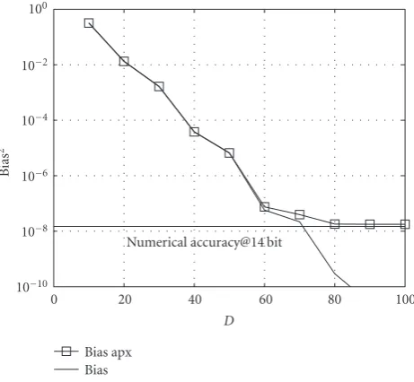
of the two-dimensional exact and the approximate DPS sub-space representation is plotted inFigure 10against the sub-space dimensionD. It can be seen that bias2hD ≈ E2max at a subspace dimension of approximately D = 80. The maxi-mum number of one-dimensional DPS vectors isD0=4 and D1=23.
4.5.2. Time, frequency, and spatial domain
Table 3contains the simulation parameters of the numerical experiments in the spatial domain. The remaining parame-ters are chosen according to Tables1and2. We assume uni-form linear arrays at the transmitter and the receiver with
100
10−2
10−4
10−6
10−8
10−10
Bi
as
2
0 20 40 60 80 100
D Numerical accuracy@14 bit
Bias apx Bias
Figure10: bias2hD for the subspace representation in the time and frequency domain withνDmax =4.82×10⁻⁵,M = 2560,θmax = 0.056, andQ=256. The resolution factors are fixed tor0 =2 and
r1 =512. The thin horizontal line denotes the numerical accuracy of a fixed-point 14-bit processor.
Table3: Simulation parameters for the numerical experiments in the spatial domains.
Parameter Value
Spacing between antennasDS λ/2 m
Number of Tx antennasNTx 8 Number of Rx antennasNRx 8 AoD interval [ϕmin,ϕmax] [−5◦, 5◦] AoA interval [ψmin,ψmax] [−5◦, 5◦] Normalized AoD bandwidthζmax−ζmin 0.087 Normalized AoA bandwidthξmax−ξmin 0.087
spacingDS =λ/2 andNTx =NRx =8 antennas each.
Fur-ther we assume that Fur-there is only one cluster of scatterers in the scenario which is not in the vicinity of the transmitter or receiver (seeFigure 11) and we assume no line-of-sight component. The AoD and AoA are assumed to be limited by [ϕmin,ϕmax]=[ψmin,ψmax]=[−5◦, 5◦], which has been ob-served in measurements [32].
A four-dimensional DPS subspace representation is ap-plied to the channel transfer function (47) withWandI de-fined in (51) and (60). Following the same procedure as in the previous subsection, for a numerical accuracy of 14 bits the estimated values of the resolution factors and the num-ber of one-dimensional DPS vectors in the spatial domains arer2=(ζmax−ζmin)/Emax≈512,r3=(ξmax−ξmin)/Emax≈
512 (rounded to the next power of 2), andD2=D3=5.
4.5.3. Hybrid DPS subspace representation
Tx Rx
Φ
Ψ
Figure11: Scenario of a mobile radio channel with one cluster of scatterers. The AoD and the AoA are limited within the intervals
Φ=[ϕmin,ϕmax] andΨ=[ψmin,ψmax], respectively.
and frequency domains, and computes the complex expo-nentials in the spatial domain directly. Therefore, the four-dimensional channel transfer functionhm (47) is split into NTxNRx two-dimensional transfer functionshsm,r describing the transfer function between transmit antennasand receiver antennar;
hsm,r:=hm,s,r=
P−1
p=0
ηpe−j2πζpsej2πξpr
! "# $
ηk,l
p
ej2πfp,m
form∈I,fp∈W,
(80)
where the band-limit region W and the index set I are the same as in the two-dimensional case (cf. (77) and (78)). Then, the two-dimensional DPS subspace representation can be applied to eachhsm,r,s=0,. . .,NTx−1,r=0,. . .,NRx−1, independently.
4.5.4. Results and discussion
A complexity comparison of the SoCE algorithm and the ap-proximate DPS subspace representation for one, two, and four dimensions is given inFigure 12. It was evaluated us-ing (70) and (73). Also shown is the complexity of the four-dimensional hybrid DPS subspace representation. It can be seen that for time-variant frequency-flat SISO channels, the one-dimensional DPS subspace representation requires fewer arithmetic operations for P > 2 MPCs. The more MPCs are used in the GCM, the more complexity is saved. Asymptotically, the number of arithmetic operations is re-duced byCh/Ch→465.
For time-variant frequency-selective SISO channels, the two-dimensional DPS subspace representation requires fewer arithmetic operations forP > 30 MPCs. However, as noted in Section 4.1, channel models for systems with the given parameters requireP = 400 paths or more. For such a scenario, the DPS subspace representation saves two orders of magnitude in complexity. Asymptotically, the number of arithmetic operations is reduced by a factor of Ch/Ch →
6.8×10³(cf. (74)). The memory requirements are Mem h= 5.83 Mbyte (cf. (75)).
For time-variant frequency-selective MIMO channels, the four-dimensional DPS subspace representation requires fewer arithmetic operations for P > 2×10³ MPCs. Since MIMO channels require the simulation of up to 104MPCs
1014
1012
1010
108
106
104
No.
o
p
er
at
io
n
s
100 101 102 103 104
P
DPSS time SoCE time DPSS time + freq. SoCE time + freq.
DPSS time + freq. + space SoCE time + freq. + space Hybrid
Figure12: Complexity in terms of number of arithmetic opera-tions versus the number of MPCsP. We show results for the SoCE algorithm (denoted by “SoCE”) and the approximate DPS subspace representation (denoted by “DPSS”) for one, two, and four dimen-sions. Also shown is the complexity of the four-dimensional hybrid DPS subspace representation (denoted by “Hybrid”).
(cf. Section 4.1), complexity savings are still possible. The asymptotic complexity savings areCh/Ch→1.9×104. How-ever, in the regionP <2×10³MPCs, the four-dimensional DPS subspace representation requires more complex oper-ations than the corresponding SoCE algorithm. Thus, even though we choose a “best case” scenario with only one clus-ter, a small angular spread and a low numerical accuracy, there is hardly any additional complexity reduction if the DPS subspace representation is applied in the spatial domain. The hybrid DPS subspace representation on the other hand exploits the savings of the DPS subspace representa-tion in the time and frequency domain only. FromFigure 12
it can be seen that it has fewer arithmetic operations than the dimensional DPS subspace representation and the four-dimensional SoCE algorithm for 60 < P < 2×10³ MPCs. Thus the hybrid method is preferable for channel simulations in this region. Further, this method also allows for an efficient parallelization on hardware channel simulators [33].
5. CONCLUSIONS
We demonstrated that the complexity reduction depends mainly on the normalized bandwidth of the underlying fad-ing process in time, frequency, and space. If the bandwidth is very small compared to the sampling rate, the essential subspace dimension of the process is small and the com-plexity can be reduced substantially. In the time domain, the maximum Doppler bandwidth of the fading process is much smaller than the system sampling rate. Compared with the SoCE algorithm, our new algorithm reduces the complexity by more than one order of magnitude on 14-bit hardware.
The bandwidth of a frequency-selective fading process is given by the maximum delay in the channel, which is a factor of five to ten smaller than the sampling rate in fquency. Therefore, the DPS subspace representation also re-duces the computational complexity when applied in the fre-quency domain. To achieve a satisfactory numerical accuracy, the resolution factor in the approximation of the basis coef-ficients needs to be large, resulting in high memory require-ments. On the other hand, it was shown that the number of memory access operations is small. Since this figure has more influence on the run-time of the algorithm, the approximate DPS subspace representation is preferable over the SoCE al-gorithm for a frequency-selective fading-process.
The bandwidth of the fading process in the spatial do-main is determined by the angular spread of the channel, which is almost as large as the spatial sampling rate for most scenarios in wireless communications. Therefore, applying the DPS subspace representation in the spatial domain does not achieve any additional complexity reduction for the sce-narios of interest. As a consequence, for the purpose of wide-band MIMO channel simulation, we propose to use a hybrid method which computes the complex exponentials in the spatial domain directly and applies the subspace represen-tation to the time and frequency domain only. This method also allows for an efficient parallelization on hardware chan-nel simulators.
APPENDICES
A. CALCULATION OF MULTIDIMENSIONAL DPS SEQUENCES
In the one-dimensional case (N = 1), whereW = [W0−
Wmax,W0+Wmax] andI= {M0,. . .,M0+M−1}, the DPS sequences can be calculated efficiently [17,20]. The efficient and numerically stable calculation of multidimensional DPS sequences with arbitraryW andIis not trivial and has not been treated satisfactorily in the literature. In this section a new way of calculating multidimensional DPS sequences is derived if their passband region can be written as a Cartesian product of one-dimensional intervals.
Indexing every elementm ∈ I lexicographically, such thatI = {ml,l=0, 1,. . .,L−1}, we define the matrixK(W)
by
Kk(W,l)=K(W)
mk−ml
, k,l=0,. . .,L−1, (A.1)
where the kernel K(W)is given by (55). Let v(d)(W,I) and λd(W,I),d=0,. . .,L−1, denote the eigenvectors and
eigen-values ofK(W):
K(W)v(d)(W,I)=λ
d(W,I)v(d)(W,I), (A.2)
where
λ0(W,I)≥λ1(W,I)≥ · · · ≥λL−1(W,I). (A.3)
It can be shown that the eigenvectors v(d)(W,I) and the eigenvaluesλd(W,I) are exactly the multidimensional DPS
vectors defined in (57) and their corresponding eigenvalues. If the DPS sequences are required form ∈/ I, they can be extended using (54).
The multidimensional DPS vectors can theoretically be calculated for an arbitrary passband regionWdirectly from the eigenproblem (A.2). However, since the matrix K(W) has an exponentially decaying eigenvalue distribution, this method is numerically unstable.
If W can be written as a Cartesian product of one-dimensional intervals (i.e.,Wis a hyper-cube),
W=W0× · · · ×WN−1, (A.4) whereWi=[W0,i−Wmax,i,W0,i+Wmax,i], and the index-set
Iis written as
I=I0× · · · ×IN−1, (A.5)
whereIi= {M0,i,. . .,M0,i+Mi−1}, the defining kernelK(W)
for the multidimensional DPS vectors evaluates to
K(W)(u)=
W0,i+Wmax,i
W0,i−Wmax,i
· · ·
W0,N−1+Wmax,N−1
W0,N−1−Wmax,N−1
e2π j f0u0
· · ·e2π j fN−1uN−1df
0 · · ·dfN−1
=
N%−1
i=0
K(Wi)u i
,
(A.6)
whereu =[u0,. . .,uN−1]T ∈ I. This means that the kernel K(W)is separable and thus the matrixK(W)can be written as a Kronecker product
K(W)=K(W0)⊗ · · · ⊗K(WN−1), (A.7)
whereK(Wi),i = 0,. . .,N−1, are the kernel matrices cor-responding to the one-dimensional DPS vectors. Now let λdi(Wi,Ii) andv(di)(Wi,Ii), di = 0,. . .,Mi−1, denote the eigenvalues and the eigenvectors ofK(Wi),i =0,. . .,N−1, respectively. Then the eigenvalues ofK(W)are given by [34, Chapter 9]
λd(W,I)=λd0
W0,I0· · ·λdN−1
WN−1,IN−1
, di=0,. . .,Mi−1, i=0,. . .,N−1