DOI : https://doi.org/10.32628/CSEIT1953162
An Efficient Method for Frequent Itemset Mining on Temporal Data
Fathima Sherin T K, Anish Kumar B.
Computer Science and Engineering, MEA Engineering College, Perinthalmanna, Kerala, India
ABSTRACT
Frequent itemset mining (FIM) is a data mining idea with extracting frequent itemset from a database. Finding frequent itemsets in existing methods accept that datasets are static or steady and enlisted guidelines are pertinent all through the total dataset. In any case, this isn't the situation when information is temporal which contains time-related data that changes data mining results. Patterns may occur during all or at specific interims, to limit time interims, frequent itemset mining with time cube is proposed to manage time arranges in the mining technique. This is how patterns are perceived that happen occasionally, in a period interim, or both. Thus, this paper mostly centres around developing up a productive calculation to mine frequent itemsets and their related time interval from a value-based database by expanding from the earlier calculation dependent on support and density as another edge. Density is proposed to deal with the overestimated timespan issue and to ensure the authenticity of the patterns found. As an extension from the current framework, here the density rate and minimum threshold is dynamically generated which is user determined parameter previously. Likewise, an analysis concerning time is made between dataset with partitioning and without apportioning the dataset, which shows computation time is less on account of partitioning technique.
Keywords : Extended Apriori Algorithm, Density, Dynamic Generation, Temporal Pattern, Frequent Itemset Mining, Time Cubes, Partitioning
I. INTRODUCTION
Data mining (sometimes referred to as data or knowledge discovery) is the way toward examining and condensing data from unique perspectives into helpful finding. In general, the path toward finding connections or patterns among wealth of fields in tremendous social databases is data mining. One of the huge endeavours in data mining is Frequent Itemset mining (FIM). The key undertaking of information mining is to investigate the database to discover consecutive, frequent patterns.
To mine knowledge from the current dataset and to transform it into the user-friendly form is the main purpose of data mining. The ability of conventional
analysis. In data mining, evaluation of Transactional data is one of the most important application.
Owing to the increase in amount of stored data, a lot of interest in the discovery of hidden information has evolved in the last ten years. This revelation has been centred for the most part around data clustering, data classification. Treating information having temporal characteristics, is a significant issue that emerges amid mining. As we know that in temporal characteristics the information is mainly related to time. These attributes need to be handled separately and differently from other attributes. Temporal information mining is a noteworthy bit of data mining. It is extraction of certain, possibly significant and heretofore unspecified information, from gigantic proportion of data. Worldly data mining manages the information mining of enormous successive informational collections. Basically, the temporal database, for the most part incorporates two mine viewpoints, valid time and transaction time. During a timespan when a reality is valid regarding this present reality then it ought to be a valid time. Transaction time is the timespan during which a reality is put away in the database.
Frequent itemset mining on temporal data is an emerging topic in data mining. Discovering frequent itemset is time consuming. To find each item in transaction along with the Time cube information is time consuming task. As of now, we understand that Frequent Itemset Mining (FIM) has been an essential bit of information investigation and information mining. FIM endeavours to extract information from databases dependent on frequently occurring events, i.e., an event, or a set of events, is interesting.
Numerous algorithms exist that performs FIM productively on distributed information, for example, Apriori. Many improved types of Apriori calculations are created as of late. In all such cases, still there are a few issues exist in frequent itemset mining, that it not
deals with huge measure of data because of higher time complexity nature. Much of the time, however, calculation ends up being immovable dependent on the user-specified threshold. To conquer these issues numerous specialists have built up an algorithm that plans to decrease generally speaking computational time. Extraction of frequent Itemset from a transaction data is a significant undertaking in information mining. The transaction entries vary periodically. Frequent Itemset mining need to be done based on temporal information. Frequent itemset mining in a ton of data is One of the critical troubles found in these days. There is need to develop effective time specific frequent Itemset extraction. Time interval specific frequent Itemset needs to be extracted from dataset.
Mining of frequent itemsets has been generally utilized in transactional databases for a considerable length of time. The traditional technique involves mining frequent itemsets on all records present at once in the transaction database. This caused performance issues such as out of memory, large computation turnaround time. The aim of the study is to propose suitable technique to overcome memory issues, reduce overall turnaround time and enable the determination of frequent itemsets based on a time frame.
The organization of this document is as follows. In Section 2 (Related Work), explains some related work done in frequent itemset mining using different methods. Section 3 (Methods and material), deals with proposed algorithm which is presented in detail. The idea of TCs is explained and the essence of a density threshold is illustrated and the partitioning approach is also discussed in detail. In Section 4 (Result and Discussion), deals with the results and a brief analysis on experimental results are described and finally in Section 5 (Conclusion), it is explained with the future scope.
II. RELATED WORK
There are lots of research work done in mining frequent itemsets using different algorithms in recent years. A Brief reviews of some of those recent significant researches are presented below:
Essalmi, Houda, et. al., [1], introduces an algorithm called, AprioriMin Algorithm which mines the frequent itemsets. This calculation goes for presenting another system for the computation of continuous itemsets to prune period of frequent itemsets. This procedure diminishes the execution time, when the support threshold increments for AprioriMin Algorithm.
Panita, Thusaranon et. al., [2], they have proposed a gradual subsistence that can deal with instance of record inclusion and cancellation all the while. The proposed algorithm predicts planned frequent itemsets by utilizing random walk procedure and update frequent itemsets when exchanges are included or erased from the database.
Moens et. al., [6], the authors used two techniques for mining frequent itemsets in parallel on the MapReduce framework where recurrence limits can be set low. First technique, called Dist-Eclat, is a pure Eclat strategy that circulates the inquiry space as equally as conceivable among mappers. This technique can mine enormous datasets, yet can be restrictive when managing massive amounts of information. In this way, present a moment, half and half strategy that first uses an Apriori based method to concentrate visit itemsets of length k and later on changes to Eclat when the projected databases fit in memory and call this calculation BigFIM.
Singh et. al., [5], expected to improve the execution of apriori algorithm by lessening the size of database and presented another characteristic Size of exchange (SOT) that takes the estimation of number of things
in individual exchange in database. The deletion process of the transaction takes place accordance to the value of k. Remove those transactions from the database only if the value of k matches with the value of SOT.
Chen et. al., [4], introduced pruned optimization strategy. With this technique, it decreases the generation of frequent itemsets and also, transaction deduction is utilized to compact the transaction of a database. The estimation of the support chose is expanding which brings about lessening number of frequent itemsets produced.
Saleh, B. and Masseglia et. al., [7], finds the subset of dataset containing more frequent itemset. For e.g. items purchasing is more in Christmas than the summer. It dynamically determines the period by analysing frequency of itemset. By traditional methods the itemset support might be less by considering the whole dataset. This technique is useful for seasonal product purchase behaviour analysis.
III. METHODS AND MATERIAL
A. Introduction
Ghorbani and Abessi [3] illustrated that when data is temporal it contains time-related information that transforms data mining results. Since information is temporal, so patterns may occur during all or few intervals, so as to confine time intervals, the algorithm called frequent itemset mining with time cubes is proposed. Time cubes are used to handle time hierarchies. This is the way patterns are recognized that occur during a particular time interval. The paper mainly focuses on developing an efficient algorithm to mine frequent itemsets and their related time interval by extending apriori based on density and support as new threshold. To deal dynamically which is user-defined parameter before. So that it will be more useful in the mining process of frequent itemsets and more effective for finding frequent itemsets. Also partitioning technique is used. Partitioning the whole dataset is done to reduce the computational time. Comparison is made between partitioning and without partitioning the dataset with respect to time where the graphs shows that the computational time is less in the case of partitioning technique.
B. Mining Frequent Patterns with Time Cubes
This section describes the methods used to mine frequent itemset mining on temporal data and also explains proposed algorithm for mining frequent itemsets.
Let I = {i1, i2, . . . in} be a set of items and C be a database of transactions. Each transaction tr is associated with an identifier transaction ID (TID), a time stamp Ttr and a set of items. For all transactions,
Ttr ϵ TS, where TS is the total time span of the hierarchy encourages us to effectively merge neighbouring frequent itemsets to discover distinctive temporal patterns. Each Time Cube represents a time interval with different time hierarchies.
For time hierarchies more than three, the term hypercube is used instead. Minimum interval is defined by the user for an equivalent length partitioning, knowing time progression and its space. These initial cubes are called Basic Time Cubes (BTCs). Since rules can occur during a very narrow time interval, it is important to specify a minimum time interval to partition the database. One can consider one hour, one day, one month to define a 1 × 1 × 1 BTC. Any two elements in BTC cannot be overlapped such that BTCi∩ BTCj = φ
Let |NCube| be the number of transactions occurred in
the cube, i.e., time interval, and | N (X)Cube | be the
number of transactions containing itemset M. The support of itemset M is calculated as follows:
Support (M) = | 𝑁 (𝑋)| 𝑁𝐶𝑢𝑏𝑒𝐶𝑢𝑏𝑒 || (1)
which contains both M and N in that time interval.
cube to the total number of transactions in that cube. So here we are increasing minimum support threshold if the transactions are more and the value is decreasing when it is less. By this way it can be generated dynamically. Since records are not equally distributed in time intervals, very few records may occur in some occasions. Therefore, discovered patterns may not be valid, since there is not enough evidence to show that they hold for the time interval. It also causes overestimating problem. So as to overcome these issues, another threshold which is called density is proposed to solve these issues. Density not only ensures the validity of the patterns as well as a channel out time interims with few records which cause overestimating the timespans.
The density of a time interval is calculated as follows: Average transaction per BTC = 𝑁
𝑁𝐵𝑇𝐶𝑠 (3)
Density = α × A (4)
where N is the all-out number of records or transactions, NBTCs is the quantity of fundamental
time cubes, therefore, A is the average transaction per BTC. α is called density rate Here we are dynamically generating α value which is introduced to determine the desired density using the equation. If the transcations are more then density rate can be decreased and if it is less, then it can be increased. In this manner, itemset is frequent if and only if for every TC, it fulfils the accompanying condition. 1) M ⟹Cube N has support greater than or equal to
the minimum threshold which is dynamically generated.
2) To ensure the validity of the rules the time interval (cube) must be dense.
Use apriori like way to find frequent itemsets in different time intervals. If an itemset M is frequent in a time interval.
1) In that time interval all subsets of M are frequent. 2) Frequent itemset M is present in all subsets of
interval.
Utilize these properties to develop an algorithm to find frequent itemsets in the transactional database. For mining frequent itemset on temporal data, it requires data with time-related information. The framework uses frequent itemset mining using time cube algorithm. The time cube algorithm is explained below:
The System uses online retail dataset as a database (C). Algorithm for Frequent Itemset Mining with Time Cubes (TCs) steps are shown below in algorithm 1. In the first step of the algorithm is uploading the database and apply preprocessing on that data. The output of the first step is pre-processed data. In third step whole pre-processed data is partitioned into number of parts. In fourth step partition database with time interval using basic time cube (BTC) value. It will partition information into used for repeat the procedure from step 5 to 7 for the entire file. Finally, it gives set of frequent itemsets with their time information.
____________________________________________ Algorithm 1 Frequent Itemsets Mining using Basic Time Cube (BTCs)
___________________________________________
Input
Database (C), Min Sup, Min den, BTC value Output
Set of frequent itemsets Method
1. Upload the dataset C
3. The whole pre-processed data is partitioned into number of parts
4. The time cube interval is taken as input by applying user-defined BTC value on C
5. Calculate support count for each candidate
6. Minimum Support Threshold is generated dynamically.
7. If Support(X) ≥ min Sup then Support is valid 8. Calculate Density as a multiplication of an average number of transactions per time interval (A) and density rate α.
9. Density rate α value is generated dynamically 10. Repeat step 5 to 7 until end of the file
11. The output is generated i.e. set of frequent itemsets with the time interval
____________________________________________
C. Enhancing Performance of the Algorithm
Finding regular itemsets is tedious on its own. yet mining designs with temporal data makes it even harder to discover an answer in a sensible time. In this way, it appears to be important to improve the exhibition of the calculation. Since density rate and minimum support threshold is user specified parameters in the existing system. But as an enhancement, we are dynamically generating these user specified parameters. This way the performance of algorithm become more effective for mining frequent itemsets.
D. System Architecture
“Fig. 1” describes the system flow. In which it contains the following modules:
1. Uploading the dataset. 2. Preprocessing the data.
3. Partition the data according to time interval defined by user.
4. Calculate the density of each time cube and filter out less than minimum.
5. Calculate the support count. 6. Obtain frequent itemsets.
Figure 1. System Flow
E. Data Specifications
Performed an experimental study to assess the performance of extended apriori algorithm. The experiment was performed on a computer with an eighth generation 64-bit Core i5 processor running Windows 10, and equipped with 701 GB of free RAM. Performance of the proposed algorithm with partitioning and without partitioning technique are compared by utilizing the given dataset. The experiment was carried out on a transactional information set containing all transactions for a UK-based and registered online retail outlet between 01/12/2010 and 09/12/2011. There are eight attributes in online retail dataset they are Invoice No, Stock Code, Description, Quantity, Invoice Date, Unit Price, Customer ID, Country. These datasets have varied characteristics such as Multivariate, Sequential and Time-Series. This online retail dataset contains 541909 instances. The dataset can be downloaded from
IV.RESULTS AND DISCUSSION
In this section experimental study is finished by way of making use of proposed algorithm. The results of proposed system based on finding frequent itemsets on temporal data and comparison of two techniques, such as partitioning and without partitioning is presented. Here apriori algorithm is extended based on support and density as a new threshold.
The exploratory investigation of the algorithm utilizing online retail dataset demonstrates that frequent itemsets are acquired in a reasonable measure of time where partitioning the whole database makes better results. Here the computation time is less because of partitioning the whole database. Density rate and minimum support threshold is user parameter before, but here it is dynamically generated which will make performance of the algorithm more efficient. The previous research didn’t focus on these user specified parameters. Also, analysis done on datasets based on time taken for both partitioning and without partitioning approach. We can see that with partitioning it will give better outcomes as the computation time is less contrasted with without partitioning.
A. Experimental Results
The implementation results can be shown as figure below:
Figure 2. Uploading the dataset
“Fig. 2” shows that the dataset file is chosen for uploading.
Figure 3. Import the dataset Market-new.csv
“Fig. 3” shows the dataset Market-new.csv is selected and uploaded.
Figure 4. Dataset is taken for preprocessing
Figure 5. Get the pre-processed data
“Fig. 5” shows that pre-processed data is obtained after removing special characters and null values.
Figure 6. Partition data according to the given time interval
“Fig 6” shows the data is partitioned according to time interval given by user.
Figure 7. The partitioned tables are viewed here by selecting each one of them
“fig 7” shows the partitioned tables which was partitioned according to user input. Each partitioned
table can be viewed here by selecting each one of them.
Figure 8. The partitioned tables are viewed whose records equal or greater than density value
“Fig. 8” shows the density is calculated for each table. If in a time cube, i.e. time interval the density rate is less than minimum density which is dynamically generated, next time cube is checked. Each table can be viewed after filter out the tables which are less than minimum density rate.
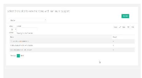
Figure 9. Selecting the tables to view the items with support count greater or equal to minimum support
“Fig. 9” shows the tables after calculating the Support count of each item. If the item has Support count less than minimum support which is also dynamically generated, item is dropped.
Figure 10. Obtain the frequent itemsets
“fig. 10” shows the frequent itemsets obtained after Partitioning the data and calculating the density value and Support of each item.
B. Comparison
TABLEI
COMPARISONRESULTSOFPARTITIONINGAND
WITHOUTPARTITIONINGTECHNIQUEDONE
ONTHEDATASET
Method Computationa
l Time
Scalabi lity
Mining Based on Time Period
Without Partitioning
High Low No
With Partitioning Technique
Medium High Yes
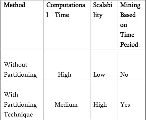
Table II above shows the comparison of two methods such as partitioning the data and without partitioning the data is taken for comparison for discovering the efficient strategy for mining frequent itemset on temporal information in a reasonable measure of time. The factors such as computational time,
scalability and mining based on time period are taken for comparison. In the case of without partitioning the data, the computational time is high and scalability is low and in this case the mining is not based on time period. We are taking the whole database for discovering frequent itemsets which is inefficient. And in the case of partitioning technique, computation time is medium and scalability is high and also mining is based on time period which is one of the efficient methods for discovering frequent itemsets.
The comparison of methods such as partitioning the data and without partitioning the data is done on the dataset. To realize which is the best strategy for frequent itemset mining. When the data is partitioned according to given time interval, it takes less time for computation. But when data is not partitioned, finding frequent itemsets become more complex. So, the algorithm is more effective in the case of using partitioning technique for finding frequent itemsets. If the computation time is less then we can mine frequent itemset effectively. Below “Fig. 11” and “Fig. 12” shows the implementation results of comparison of two methods.
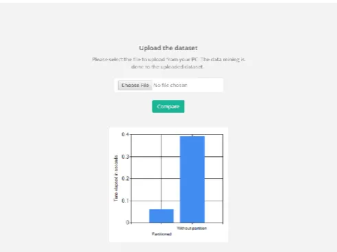
Figure 11. Uploading the dataset Market.csv for comparison
Figure 12. Obtain the graph which shows time taken (in sec) for partitioning and without partitioning data
“Fig. 12” shows the Graph obtained which shows time taken (in sec) after the comparison between the partitioning and without partitioning the data.
V. CONCLUSION
The paper mainly concentrates on developing an efficient algorithm for mining frequent itemset by extending apriori and gives frequent itemset along with time related data as output. And also focuses on limitation of existing system, where density rate and minimum support threshold are given by the user, but in this paper, they are dynamically generated which will make frequent itemset mining more efficient. Also, comparison of two methods such as partitioning and without partitioning technique is done on dataset with respect to time. Partition technique, which shows less computation time is taken when partition is done to dataset than without partitioning. So, calculation time is less in mining frequent itemsets when partition procedure is utilized. For future work, enhance performance of the algorithm by using multithreaded processors such as graphic processing units to speed up the computations.
VI.REFERENCES
[1] Essalmi, Houda, et al. "A novel approach for mining frequent itemsets: AprioriMin." 2016 4th IEEE International Colloquium on
Information Science and Technology (CiSt).
IEEE, 2016.
[2] Thusaranon, Panita, and Worapoj Kreesuradej. "Frequent itemsets mining using random walks for record insertion and deletion." In 2016 8th International Conference on Information
Technology and Electrical Engineering
(ICITEE), pp. 1-6. IEEE, 2016.
[3] Ghorbani, Mazaher, and Masoud Abessi. "A new methodology for mining frequent itemsets on temporal data." IEEE Transactions on
Engineering Management 64.4 (2017): 566-573.
[4] Chen, Zhuang, et al. "An improved Apriori algorithm based on pruning optimization and transaction reduction." 2011 2nd International
Conference on Artificial Intelligence,
Management Science and Electronic Commerce
(AIMSEC). IEEE, 2011.
[5] Singh, Jaishree, Hari Ram, and Dr JS Sodhi. "Improving efficiency of apriori algorithm using transaction reduction." International
Journal of Scientific and Research
Publications3.1 (2013): 1-4.
[6] Moens, Sandy, Emin Aksehirli, and Bart Goethals. "Frequent itemset mining for big data." In 2013 IEEE International Conference
on Big Data, pp. 111-118. IEEE, 2013.
[7] Saleh, Bashar, and Florent Masseglia. "Discovering frequent behaviors: time is an essential element of the context." Knowledge
and Information Systems 28, no. 2 (2011):
Cite this article as :