DINOVA, VINCENT ANTHONY. Automated Variable Selection of Gamma-Ray Spectra by Utilization of LASSO and Elastic Net Techniques for Use in Nuclear Security Applications. (Under the direction of Dr. Robin Gardner).
In the aftermath of the disasters of September 11th, 2001, new security measures were
taken to prevent future attacks. Due to the extreme destructive physical and psychological power of nuclear weapons and radiation dispersal devices, a large effort has been spent in preventing the proliferation of nuclear weapons and materials. Soft targets, such as oil well logging radiochemical sources, have been identified as a commonly used radioactive source that can be replaced by non-active sources such as D-T or D-D pulsed neutron generators.
An experiment at Kansas State University was conducted, using a D-T pulsed neutron generator and test facility to replicate different scenarios commonly found in oil wells. D-T pulsed neutron generators have the ability to generate neutrons at a comparable rate to AmBe and Cf-252 neutron sources. These neutrons then bombard surrounding materials to release gamma rays by inelastic scattering and absorption commonly referred to as prompt gamma neutron activation analysis. D-T pulsed neutron generators produce neutrons at a higher energy than traditional sources, allowing for additional inelastic scattering schemes to be unlocked. Additionally, pulse timing sequences can be manipulated utilizing a digitizer to separate prompt and delayed responses.
This dissertation is devoted to investigating new supervised machine learning algorithms, LASSO and Elastic Net, that are used to automatically perform variable selection and model prediction. MCNP generated libraries are simulated to estimate the detector response using the geometry and material composition of the tool, testing chamber, and surrounding materials and compared to experiments performed at Kansas State University.
© Copyright 2019 by Vincent DiNova
by
Vincent A. DiNova, Jr.
A dissertation submitted to the Graduate Faculty of North Carolina State University
in partial fulfillment of the requirements for the degree of
Doctor of Philosophy
Nuclear Engineering
Raleigh, North Carolina 2019
APPROVED BY:
_______________________________ _______________________________ Dr. Robin Gardner Dr. Steven Shannon
Committee Chair
DEDICATION
BIOGRAPHY
Vincent DiNova was born in Orlando, Florida and traveled the world as the son of a naval officer. After completing high school at Apex High School, he went on to study Nuclear
ACKNOWLEDGMENTS
There are so many people who have impacted me on this journey, I hope to capture them all, and I sincerely apologize if I forget any single person. If you read this and think you should have been listed here, believe me that although you are not listed, your impact has been noticed.
The people who have had the largest impact on my life and subsequent work are my family. To my mother and father, Vince and Kay, you have inspired me to be the best man I can be and to push myself to continue to improve every day. To my sister, Kristina, my brother-in-law, Tommy, and my nephew, Jack, my aunts and uncles, Karen, Joe, Nico and Lisa, my memaw and pepaw, and to all my cousins, you have all given me inspiration, examples to follow, and much help when needed. I thank and love you all.
To all my childhood friends who helped shape who I am. I want to especially
acknowledge my wonderful friends from Apex High School and their families: Sean Roberts, Matt Baldiga, Kyle Beaulieu, Charlotte Florez, Jill Nee, Nancy Andrews, Darah Willey, Vicki Tucci, Hanna Zombek, Claire Wagner, Gina Winters, Heather Copley, Meredith Caley, Christine Reed, Stephen Mason, and Jenna Ready. All of you helped bring me out of my shell and gain confidence in myself. You and your families became family to me, I think of you all often, and I want you to know I would not have made it here without meeting each of you.
So many people helped me out during my undergraduate degree. To all my professors: Dr. Bourham, Dr. Hawari, Dr. Hankins, Dr. Anistratov, Dr. Doster, and Dr. Turinsky, you all gave me the skills I needed to carry forward to this point. To my classmates, thank you for making life more enjoyable during that period, especially, Aimee Smith, Alison Koeppel, Richard Mongold, Jay Alexander, and Chris Courtenay.
To all of the NC State bowling team, thank you for giving me the best times of my life. I especially want to thank Zack Brown, Jon Scorano, Nick Davis, Brian James, Wes Wheless, Eric Moore, Mike Flitcraft, Rachel Judd, AJ Van Fleet, Kyle Burns, and Craig Nursey. To our coach Irwyn Atkinson, who spent over 30 years coaching the NC State bowling team, you deserve to be immortalized in this work for the contribution you have made to the university and on my life. I thank you for your friendship and mentorship.
can. You have been tremendous friends for so long, and I thank you for all of your help over the years.
To all my peers during graduate school, you have all made these years fun and exciting. I especially want to thank Wes Holmes, Aaron Feinberg, Richard Howard, James Gilman, Adan Calderon, Sean O’brien, Brandon Burns, Andrew Petrarca, Josh Novak, Kyoung Lee, Mario Milev, and Rob Weldon.
To the friends and coworkers I met during my time at Bechtel, for providing me with professional and personal growth, I thank you. I especially want to thank Sarah Fafard, Fotios Raftelis, Hagan Baturay, Dave Dinse, Evan Fredo, Summar Sammons, Hailey Clark, Jimmy and Candi Coble, Stephanie Quinn, Sam Watson, Grant Whitfield, Thomas Ramis, Dan Triplett, and Kenny Hearn.
There are a few people who helped keep me focused during my return to graduate school, Ashley Stancil and her family, Dara O’Sullivan, Rachel Helscher, and Kim Nguyen-Dinh. I thank you for all keeping me on a path that has led me here.
To the NNSA for funding this project and work, and those that helped run the program. I especially want to thank Dr. Mattingly, Dr. Azmy, Stefani Buster, and Russell Villard for
helping keep the consortium on track.
To the CNEC students and faculty for their help and support on this project. I especially want to acknowledge Dr. Bill Dunn and Dr. Walter McNeil for setting up the experiment that generated the data used for this project, as well as their students Long Vo, Maria Pinella, Diego Laramore, and Aaron Hellinger.
To Lisa Marshall, for being a great friend and for all the continued excellence you bring to the department and American Nuclear Society.
To my new family, Speed and Stevie, you give me the motivation to be the best I can be. This is as much for you, as any other person. I love you both.
TABLE OF CONTENTS
LIST OF TABLES ... ix
LIST OF FIGURES ... xi
Chapter 1: Introduction ... 1
1.1 Background ... 1
1.2 Benchmarking Tool and Facility ... 3
1.3 Monte Carlo Library Least Squares ... 5
1.4 Radioisotope Identification Devices ... 6
Chapter 2: Nuclear Reactions ... 8
2.1 Neutron Transport ... 8
2.1.1 Neutron Inelastic Scatter (n, n’γ) ... 8
2.1.2 Neutron Capture (n, γ) ... 9
2.2 Photon Transport ... 10
2.3 Detector Response ... 13
2.3.1 Spectral Features ... 13
Chapter 3: Machine Learning Enhancements ... 18
3.1 Supervised Machine Learning ... 18
3.1.1 Linear Least Squares ... 18
3.1.2 Least Absolute Selection and Shrinkage Operator (LASSO) ... 19
3.1.3 Elastic Net ... 20
3.1.4 Coordinate Descent Solutions for LASSO and Elastic Net ... 21
3.1.4.1 LASSO Singe Variable Case ... 22
3.1.4.2 Coordinate Descent for LASSO ... 23
3.1.4.3 Coordinate Descent for Elastic Net ... 25
3.1.5 Cross Validation... 27
Chapter 4: Kansas State Experiment ... 29
4.1 Data Collection ... 29
4.1.1 Kansas State Experimental Data ... 29
4.1.2 Simulated Data ... 30
4.1.3 Simulated Example ... 30
4.2 Methods and Improvements ... 34
4.2.1 Full Procedure ... 34
4.2.2 Early Lessons Learned ... 35
4.3 Kansas State Experimental Results ... 38
4.3.1 Water Trial ... 39
4.3.2 Sand Trial ... 50
4.3.3 Sand with Water Trial ... 61
4.3.4 Limestone Trial ... 72
4.3.5 Limestone with Water Trial ... 83
Chapter 5: Radioisotope Identification Device Algorithm... 95
5.1 Data Collection ... 95
5.2 Masking Without Shielding ... 96
5.3 Convolution Without Shielding ... 101
5.4 Masking with Shielding ... 105
5.5 Convolution with Shielding ... 109
Chapter 6: Discussion and Conclusions ... 114
References ... 116
Appendices ... 119
Appendix A: MCNP Sample Deck – KSU Application ... 120
Appendix B: LASSO Code Sample ... 125
LIST OF TABLES
Table 1-1: NAS findings ... 1
Table 2-1: Non-elastic scattering reactions and threshold energies ... 9
Table 3-1: Full LASSO Coordinate Descent Algorithm ... 25
Table 3-2: Full Elastic Net Coordinate Descent Algorithm ... 27
Table 4-1: Relative error of the two methods ... 34
Table 4-2: Optimal normalization parameters for water trial ... 47
Table 4-3: Linear coefficients and error for water near detector ... 49
Table 4-4: Linear coefficients and error for water far detector ... 50
Table 4-5: Optimal normalization parameters for sand trial ... 59
Table 4-6: Linear coefficients and error for sand near detector ... 61
Table 4-7: Linear coefficients and error for sand far detector ... 61
Table 4-8: Optimal normalization parameters for sand and water trial ... 70
Table 4-9: Linear coefficients and error for sand and water near detector ... 72
Table 4-10: Linear coefficients and error for sand and water far detector ... 72
Table 4-11: Optimal normalization parameters for limestone trial ... 81
Table 4-12: Linear coefficients and error for limestone near detector ... 83
Table 4-13: Linear coefficients and error for limestone far detector ... 83
Table 4-14: Optimal normalization parameters for limestone and water trial ... 92
Table 4-15: Linear coefficients and error for limestone and water near detector ... 94
Table 4-16: Linear coefficients and error for limestone and water far detector ... 94
Table 5-1: Masking coefficients and total count ... 97
Table 5-3: Convolution coefficients and total counts ... 101
Table 5-4: Convolution trial prediction accuracy for LASSO and Elastic Net
with varying count rates ... 105
Table 5-5: Masking with shielding coefficients and total counts ... 106
Table 5-6: Masking with shielding trial prediction accuracy for LASSO and Elastic Net
with varying count rates ... 109
Table 5-7: Convolution with shielding coefficients and total counts ... 110
Table 5-8: Convolution with shielding trial prediction accuracy for LASSO
LIST OF FIGURES
Figure 1-1: Prompt and delayed gamma ray emission process ... 2
Figure 1-2: KSU benchmarking tool ... 3
Figure 1-3: Data acquisition scheme ... 3
Figure 1-4: KSU design facility ... 4
Figure 1-5: Test chamber ... 4
Figure 1-6: a. Open borehole tube, b. Capped borehole tube ... 5
Figure 2-1: Depiction of the Photoelectric Effect ... 10
Figure 2-2: Depiction of the Compton Scattering process ... 11
Figure 2-3: Illustration of the Compton edge and continuum ... 11
Figure 2-4: Depiction of interaction of gamma-rays with a detector medium and their resultant spectra ... 12
Figure 2-5: Energy dependence of photon interactions in NaI ... 13
Figure 2-6: Infinite resolution detector response ... 14
Figure 3-1: Soft-thresholding function ... 22
Figure 3-2: Holdout method for test-train split ... 28
Figure 3-3: Cross validation holdout ... 28
Figure 4-1: F8 tally simulated response and Gaussian broadened detector response ... 30
Figure 4-2: Cross validation normalization parameter selection for LASSO ... 31
Figure 4-3: LASSO model selection coefficients by changing normalization parameter ... 31
Figure 4-4: LASSO salt water simulation fit ... 32
Figure 4-5: Cross validation normalization parameter selection for Elastic Net ... 32
Figure 4-6: Elastic Net model selection by changing normalization parameter ... 33
Figure 4-8: Full procedure ... 35
Figure 4-9: Pure water first fit ... 36
Figure 4-10: Pure water fit with NaI activation libraries added ... 36
Figure 4-11: Firing sequence and measured response ... 37
Figure 4-12: Time dependent format distributed by Kansas State University ... 38
Figure 4-13: Cross validation normalization parameter selection for the LASSO near detector water trial ... 39
Figure 4-14: LASSO model selection coefficients by changing the normalization parameter for the near detector water trial ... 40
Figure 4-15: LASSO fit for the near detector water trial ... 40
Figure 4-16: LASSO full fit for the near detector water trial ... 41
Figure 4-17: Cross validation normalization parameter selection for the Elastic Net near detector water trial ... 41
Figure 4-18: Elastic Net model selection coefficients by changing the normalization parameter for the near detector water trial ... 42
Figure 4-19: Elastic Net fit for the near detector water trial ... 42
Figure 4-20: Elastic Net full fit for the near detector water trial ... 43
Figure 4-21: Cross validation normalization parameter selection for the LASSO far detector water trial ... 43
Figure 4-22: LASSO model selection coefficients by changing the normalization parameter for the far detector water trial ... 44
Figure 4-23: LASSO fit for the far detector water trial ... 44
Figure 4-24: LASSO full fit for the far detector water trial ... 45
Figure 4-25: Cross validation normalization parameter selection for the Elastic Net far detector water trial ... 45
Figure 4-27: Elastic Net fit for the far detector water trial ... 46
Figure 4-28: Elastic Net full fit for the far detector water trial ... 47
Figure 4-29: Linear least squares fit and residual for the near detector water trial ... 48
Figure 4-30: Linear least squares fit and residual for the far detector water trial ... 48
Figure 4-31: Linear least squares fit for near and far detector water trials ... 49
Figure 4-32: Cross validation normalization parameter selection for the LASSO near detector sand trial ... 51
Figure 4-33: LASSO model selection coefficients by changing the normalization parameter for the near detector sand trial ... 51
Figure 4-34: LASSO fit for the near detector sand trial ... 52
Figure 4-35: LASSO full fit for the near detector sand trial ... 52
Figure 4-36: Cross validation normalization parameter selection for the Elastic Net near detector sand trial ... 53
Figure 4-37: Elastic Net model selection coefficients by changing the normalization parameter for the near detector sand trial ... 53
Figure 4-38: Elastic Net fit for the near detector sand trial ... 54
Figure 4-39: Elastic Net full fit for the near detector sand trial ... 54
Figure 4-40: Cross validation normalization parameter selection for the LASSO far detector sand trial ... 55
Figure 4-41: LASSO model selection coefficients by changing the normalization parameter for the far detector sand trial ... 55
Figure 4-42: LASSO fit for the far detector sand trial ... 56
Figure 4-43: LASSO full fit for the far detector sand trial ... 56
Figure 4-44: Cross validation normalization parameter selection for the Elastic Net far detector sand trial ... 57
Figure 4-46: Elastic Net fit for the far detector sand trial ... 58
Figure 4-47: Elastic Net full fit for the far detector sand trial ... 58
Figure 4-48: Linear least squares fit and residual for the near detector sand trial ... 59
Figure 4-49: Linear least squares fit and residual for the far detector sand trial ... 60
Figure 4-50: Linear least squares fit for near and far detector sand trials ... 60
Figure 4-51: Cross validation normalization parameter selection for the LASSO near detector sand and water trial ... 62
Figure 4-52: LASSO model selection coefficients by changing the normalization parameter for the near detector sand and water trial ... 62
Figure 4-53: LASSO fit for the near detector sand and water trial ... 63
Figure 4-54: LASSO full fit for the near detector sand and water trial ... 63
Figure 4-55: Cross validation normalization parameter selection for the Elastic Net near detector sand and water trial ... 64
Figure 4-56: Elastic Net model selection coefficients by changing the normalization parameter for the near detector sand and water trial ... 64
Figure 4-57: Elastic Net fit for the near detector sand and water trial ... 65
Figure 4-58: Elastic Net full fit for the near detector sand and water trial ... 65
Figure 4-59: Cross validation normalization parameter selection for the LASSO far detector sand and water trial ... 66
Figure 4-60: LASSO model selection coefficients by changing the normalization parameter for the far detector sand and water trial ... 66
Figure 4-61: LASSO fit for the far detector sand and water trial ... 67
Figure 4-62: LASSO full fit for the far detector sand and water trial ... 67
Figure 4-63: Cross validation normalization parameter selection for the Elastic Net far detector sand and water trial ... 68
Figure 4-65: Elastic Net fit for the far detector sand and water trial ... 69
Figure 4-66: Elastic Net full fit for the far detector sand and water trial ... 69
Figure 4-67: Linear least squares fit and residual for the near detector sand and water trial ... 70
Figure 4-68: Linear least squares fit and residual for the far detector sand and water trial ... 71
Figure 4-69: Linear least squares fit for near and far detector sand and water trials ... 72
Figure 4-70: Cross validation normalization parameter selection for the LASSO near detector limestone trial ... 73
Figure 4-71: LASSO model selection coefficients by changing the normalization parameter for the near detector limestone trial ... 73
Figure 4-72: LASSO fit for the near detector limestone trial ... 74
Figure 4-73: LASSO full fit for the near detector limestone trial ... 74
Figure 4-74: Cross validation normalization parameter selection for the Elastic Net near detector limestone trial ... 75
Figure 4-75: Elastic Net model selection coefficients by changing the normalization parameter for the near detector limestone trial ... 75
Figure 4-76: Elastic Net fit for the near detector limestone trial ... 76
Figure 4-77: Elastic Net full fit for the near detector limestone trial ... 76
Figure 4-78: Cross validation normalization parameter selection for the LASSO far detector limestone trial ... 77
Figure 4-79: LASSO model selection coefficients by changing the normalization parameter for the far detector limestone trial ... 77
Figure 4-80: LASSO fit for the far detector limestone trial ... 78
Figure 4-81: LASSO full fit for the far detector limestone trial ... 78
Figure 4-82: Cross validation normalization parameter selection for the Elastic Net far detector limestone trial ... 79
Figure 4-84: Elastic Net fit for the far detector limestone trial ... 80
Figure 4-85: Elastic Net full fit for the far detector limestone trial ... 80
Figure 4-86: Linear least squares fit and residual for the near detector limestone trial ... 81
Figure 4-87: Linear least squares fit and residual for the far detector limestone trial ... 82
Figure 4-88: Linear least squares fit for near and far detector limestone trials ... 82
Figure 4-89: Cross validation normalization parameter selection for the LASSO near detector limestone and water trial ... 84
Figure 4-90: LASSO model selection coefficients by changing the normalization parameter for the near detector limestone and water trial ... 84
Figure 4-91: LASSO fit for the near detector limestone and water trial ... 85
Figure 4-92: LASSO full fit for the near detector limestone and water trial ... 85
Figure 4-93: Cross validation normalization parameter selection for the Elastic Net near detector limestone and water trial ... 86
Figure 4-94: Elastic Net model selection coefficients by changing the normalization parameter for the near detector limestone and water trial ... 86
Figure 4-95: Elastic Net fit for the near detector limestone and water trial ... 87
Figure 4-96: Elastic Net full fit for the near detector limestone and water trial ... 87
Figure 4-97: Cross validation normalization parameter selection for the LASSO far detector limestone and water trial ... 88
Figure 4-98: LASSO model selection coefficients by changing the normalization parameter for the far detector limestone and water trial... 88
Figure 4-99: LASSO fit for the far detector limestone and water trial ... 89
Figure 4-100: LASSO full fit for the far detector limestone and water trial ... 89
Figure 4-101: Cross validation normalization parameter selection for the Elastic Net far detector limestone and water trial ... 90
Figure 4-103: Elastic Net fit for the far detector limestone and water trial ... 91
Figure 4-104: Elastic Net full fit for the far detector limestone and water trial ... 91
Figure 4-105: Linear least squares fit and residual for the near detector limestone and water trial ... 92
Figure 4-106: Linear least squares fit and residual for the far detector limestone and water trial ... 93
Figure 4-107: Linear least squares fit for near and far detector limestone and water trials ... 93
Figure 5-1: Vised depiction of detector geometry ... 96
Figure 5-2: MCNP generated radioisotope libraries ... 96
Figure 5-3: LASSO masking low count rate fit ... 97
Figure 5-4: Elastic Net masking low count rate fit ... 98
Figure 5-5: LASSO masking medium count rate fit ... 98
Figure 5-6: Elastic Net masking medium count rate fit ... 99
Figure 5-7: LASSO masking high count rate fit ... 99
Figure 5-8: Elastic Net masking high count rate fit ... 100
Figure 5-9: LASSO convolution low count rate fit ... 102
Figure 5-10: Elastic Net convolution low count rate fit ... 102
Figure 5-11: LASSO convolution medium count rate fit ... 103
Figure 5-12: Elastic Net convolution medium count rate fit ... 103
Figure 5-13: LASSO convolution high count rate fit ... 104
Figure 5-14: Elastic Net convolution high count rate fit ... 104
Figure 5-15: LASSO masking with shielding low count rate fit ... 106
Figure 5-16: Elastic Net masking with shielding low count rate fit ... 107
Figure 5-18: Elastic Net masking with shielding medium count rate fit ... 108
Figure 5-19: LASSO masking with shielding high count rate fit ... 108
Figure 5-20: Elastic Net masking with shielding high count rate fit ... 109
Figure 5-21: LASSO convolution with shielding low count rate fit ... 110
Figure 5-22: Elastic Net convolution with shielding low count rate fit ... 111
Figure 5-23: LASSO convolution with shielding medium count rate fit ... 111
Figure 5-24: Elastic Net convolution with shielding medium count rate fit ... 112
Figure 5-25: LASSO convolution with shielding high count rate fit ... 112
CHAPTER 1
Introduction
1.1 Background
Shortly after the tragedies of September 11, 2001, the National Academies of Science
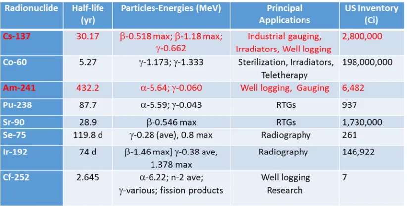
commissioned a study on the dangers of long-lived radioisotope sources. The study concluded that there exist several commonly used sources that could potentially be used as a dirty bomb or terror weapon (Table 1-1). The Consortium for Nonproliferation Enabling Capabilities (CNEC) was funded in 2014 to research innovative ways to address nuclear security problems including finding suitable replacements for dangerous radiological sources.
Table 1-1: NAS findings
firing sequence that propels Deuterons and Tritons on a collision path releasing 14.1 MeV neutrons. These high-energy neutrons are used as an alternative to AmBe neutrons in a traditional prompt gamma neutron activation analysis (PGNAA) application. PGNAA is a nondestructive method that relies on (n, γ) neutron capture, and (n, n’γ) neutron inelastic
scattering reactions to produce gamma photons, each having distinct characteristics of the target nuclei. Using a near and far NaI scintillator detector, each spectral detector response can be analyzed for elemental composition.
PGNAA suffers from a low signal to noise ratio caused by the delayed activation of nuclei or neutron activation analysis (NAA). Neutron activation analysis utilizes the delayed gamma rays from radioactive daughters, while PGNAA exploits the prompt gamma rays (Fig. 1-1). The neutron cross sections for both prompt and delayed reactions compete and create a mixed signal that is often difficult to process. Additional sources of interference include:
1) γ rays produced by the PNG
2) γ rays from activation inside the detector medium (Gardner, 2000) 3) γ rays from background sources
4) γ rays produced by the activation of construction materials in the benchmarking tool.
Figure 1-1: Prompt and delayed gamma ray emission process
The PNG offers a unique solution to this problem by exploiting the pulsing time responses with a digitizer allowing the prompt and delayed responses to be extracted and
1.2 Benchmarking tool and facility
The benchmarking tool and design facility were designed and constructed at Kansas State
University. The tool consists of near and far gamma and neutron detectors separated from a D-T PNG source by a 2” lead divider (Fig. 1-2). A CAEN 5730 digitizer acts to both send the pulse firing sequence to the PNG and to collect the responses from the gamma and neutron detectors (Fig. 1-3).
Figure 1-2: KSU benchmarking tool
Figure 1-3: Data acquisition scheme
Figure 1-4: KSU design facility
The test chamber (Figs. 1-5, 1-6) is 6’8” high by 6’6” wide and 8’ deep with a total volume of roughly 2,500 gallons. These dimensions ensure that when fully filled with water, the test chamber presents an effectively infinite medium to the 14.1 MeV neutrons. During the data collection process, the benchmarking tool is loaded into the borehole tube and enclosed by a cap. Borated polyethylene (green material) has been fitted both inside and outside the test chamber to reduce neutron escape and dosage.
Figure 1-6: a. Open borehole tube b. Capped borehole tube
1.3 Monte Carlo Library Least Squares
In order to quantitatively analyze measured PGNAA γ spectra, Monte Carlo Library Least Squares (MCLLS) has been shown to be an effective method over single peak analysis (Gardner, 1997). MCLLS requires extremely accurate forward model simulations to represent the expected pulse-height spectrum obtained with a PGNAA system with a known geometry and
compositional makeup. Previous studies have demonstrated the effectiveness on bulk coal (Shyu et al., 1988, 1998) and PGNAA applications (Han, 2005 and Hou, 2017). The MCLLS approach consists of:
1) Generating pulse-height spectra with MCNP or similar coding packages using assumed or known geometry and compositions.
2) Utilizing each prompt γ-ray pulse-height spectrum as a library input variable for model selection.
3) Adjusting all non-linear parameters between simulated and experimental response to treat the problem as a sum of linear responses.
4) Perform a linear library least-squares (LLS) analysis.
Assuming all non-linear physical components are correctly adjusted, the library least-squares method treats an unknown sample as the sum of the products of an elemental amount with the library spectrum of each element for each channel as given by equation 1.1.
Where,
• 𝑦 is the counts per channel 𝑖 of an unknown spectrum
• 𝑎 are linear coefficients for each element 𝑗
• 𝑥 are the library spectra, or counts in channel 𝑖 of element 𝑗
• 𝑒 is random error in counts in channel 𝑖
Equation 1.1 is solved for 𝑥 by minimizing the reduced Chi-Square 𝜒 given by equation 1.2.
𝜒 𝑒
𝑛 𝑚 𝜎
(1.2)
Where,
• 𝑛 𝑚 is the number of degrees of freedom
• 𝑒 is random error in counts in channel 𝑖
• 𝜎 is the variance of the random error in counts in each channel i
1.4 Radioisotope Identification Devices
During this investigation using LASSO and Elastic Net variable selection techniques on oil well logging devices, radioisotope identification devices (RIIDs) were targeted as another application that could be improved by the use of these algorithms. RIIDs are handheld instruments designed to identify radioactive materials by their emitted gamma ray energies. RIID algorithm
development is necessary to ensure that potential threats are correctly identified by field agents and first responders. A study from 2003 concluded that only 30%-50% of medical, industrial, NORM, and threat isotopes were correctly identified (Blackadar et. al).
RIID algorithms measure similarities between measured characteristics of test spectrum and reference spectra, whether experimental or simulated. Many challenges emerge as a result of variations that occur naturally (Burr and Hamada, 2009) including:
Voltage calibrations can be nonlinear, and electronic gain shift effects can be nonlinear and unstable over time due to environmental effects.
Procedural protocols can complicate the required measurements. Temperature and spatial factors can impact the calibration and collection time necessary to collect accurate measurements.
There can be hundreds of isotopes in the isotope library, each with numerous example spectra.
Detector dead time and pulse pile up can distort the test spectra.
CHAPTER 2
Nuclear Reactions
Prompt gamma-ray neutron activation analysis (PGNAA) is a nondestructive, near real time technique used for bulk material identifications. PGNAA relies on neutron inelastic scatter and capture reactions to produce characteristic γ-rays used to identify minute amounts of elements in a bulk sample. Due to low cross sections for these reactions, background sources from natural radiation, activation of the NaI detector, and γ-rays from the decay of the neutron source a low signal to noise ratio (SNR) is common.
2.1 Neutron Transport
There are a number of different mechanisms by which neutrons can interact with nuclei. For the prompt gamma neutron activation analysis application, only two are considered.
2.1.1 Neutron Inelastic Scatter (n, n’γ)
Neutron inelastic scatter involves an incoming neutron colliding with a target nucleus and exiting with less energy and at a different angle than it entered. The energy deposited on the target nucleus causes it to reach an excited state and rapidly releases a γ-ray to return to its normal energy state represented in equation 2.1 as follows:
𝑛 𝑋 → 𝑛 𝑋∗ (2.2)
The inelastic scattering reaction requires an incoming neutron to have enough energy to
break the threshold energy derived from the Q value formula shown in equation 2.2.
𝑇 𝐸 𝐴 1
𝐴
Where,
• 𝑇 is the kinetic energy of the incident neutron
• 𝐸 is the energy of the target nucleus’ first excited level
• 𝐴 is the atomic number of the target nucleus
The PNG is advantageous for this decay scheme, as the 14.1 MeV neutrons allow a greater number of isotopes to undergo inelastic scattering and unlock higher energy states. Table 2-1 (Kim et, al. 2006) below lists some common inelastic scatter threshold energies and cross sections.
Table 2-1: Non-elastic scattering reactions and threshold energies
2.1.2 Neutron Capture (n, γ)
Neutron capture, also denoted as (n, γ), can occur over a wide range of energies and has the highest probability at thermal energies. The (n, γ) reaction begins when a neutron interacts with a target nucleus and is absorbed. The newly formed nucleus is placed in an excited state, and in order to form a new ground state, at least one γ photon is emitted as shown in eq. 2.3 below.
𝑛 𝑋 → 𝑋∗ (2.3)
2.2 Photon Transport
2.2.1 Photon Reactions
The benchmarking tool analysis relies on three main photon reactions: photoelectric absorption, Compton scattering, and pair production. Although there are other photon reactions, none are an important focus to this work.
Photoelectric Absorption
During photoelectric absorption, a photon interacts with a target atom’s electron, departs all of its energy, disappears, and ejects the electron from its bound shell. The photoelectron carries an energy given by equation 2.4 and illustrated by figure 2-1.
𝐸 ℎ𝑣 𝐸 (2.4)
Where,
• 𝐸 is the binding energy of the photoelectron in its original shell
• 𝐸 is the energy of the exited photoelectron
• ℎ𝑣 is the energy of the incoming photon
Figure 2-1: Depiction of the Photoelectric Effect
Compton Scattering
𝐸′ 𝐸
1 1 𝑐𝑜𝑠𝜃 𝐸 /𝑚 𝑐
(2.5)
Where,
• 𝐸′ is the scattered photon energy
• 𝐸 is the energy of the incident photon
• 𝑐𝑜𝑠𝜃 is the scattering angle in the lab frame
• 𝑚 is the mass of the electron
• 𝑐 is the speed of light
Figure 2-2: Depiction of the Compton Scattering process
Figure 2-3: Illustration of the Compton edge and continuum
Pair Production
Figure 2-5: Energy dependence of photon interactions in NaI
2.3 Detector Response
Incident radiation interacting with the detector are modeled in MCNP 6.1 and carry distinct physical signatures (Knoll, 2011). The first order physics alone do not provide a genuine representation of the response from a detector. In order to accurately reproduce a detector response, a detector response function (DRF) must be applied. A detector response function is the expected detector response provided an incoming particle (Gardner and Sood, 2004). During this stage, all non-linear characteristics are removed, allowing the problem to be solved by linear methods.
2.3.1 Spectral Features
Figure 2-6: Infinite resolution detector response
A: Full Energy Peak
The full energy peak is equal to the incoming photon energy, 6.13 MeV for this example. The pulse signals that produce this signature occur when the particle enters the detector and deposits all its energy with no escaping secondary particles. This can occur in a singular photoelectric absorption or by a series of reactions. For this reason, the full energy peak can be referred to as the “photoelectric peak”.
B: Compton Edge
Not all events result in full energy deposition. The Compton edge occurs once a photon undergoes a Compton scattering reaction, and then exits the detector without depositing additional energy. The scattering angle determines the energy that is deposited in the detector, ranging from 0° to 180°. From equation 2.6, the maximum energy deposited by a Compton scattering identified as the Compton edge is
𝛥𝐸 𝐸 𝐸 6.13 6.13
1 1 𝑐𝑜𝑠𝜋 ∗ 6.130.511 5.88 MeV
(2.6) A
G
E
F
D C
C: Single Escape Peak
In the event a photon creates a pair production reaction, an electron-positron pair is created. The positron will then annihilate inside the detector, creating a 0.511 MeV photon. If the annihilation photon exits the detector without depositing its energy and the full energy of the incoming
photon is deposited inside the detector, the result is the single escape peak. The energy of the peak is equal to the full energy peak minus the resting mass energy of an electron, 0.511 MeV.
D: Double Escape Peak
The double escape peak is the result of both annihilation photons escaping the detector. As a result, the detected energy is equal to that of the full energy peak minus the resting mass energy of two electrons, 1.022 MeV.
E: Annihilation Peak
In the event that the incoming particle interacts with a material outside of the detector by a pair production reaction, a resulting annihilation photon can enter the detector and deposit its energy. The annihilation peak appears when the detector is surrounded by a dense material and is equal to 0.511 MeV.
F: Backscattering Peak
The backscattering peak is created when a Compton scattering event occurs outside the detector and the scattered photon reaches the detector and deposits its full energy. The scattering angle occurs over a small range of angles around 180°. This causes the peak to be a range of energies instead of a singular energy peak. The energy for backscattering peak is usually between 200 and 300 KeV. For the case of 180° scatter, the energy of the incoming scattered photon would be
𝐸 6.13
1 1 𝑐𝑜𝑠𝜋 ∗ 6.130.511 0.245 MeV
(2.7)
G: X-Ray Fluorescence Peaks
generated by interactions that occur in the surrounding medium by exciting the target atom. During the de-excitation, characteristic X-ray photons are emitted and enter the detector and deposit their full energy. These peaks complicate the fitting functions, as they can be orders of magnitude higher than other signatures within the spectrum.
H: X-Ray Escape Peaks
When the excited atoms discussed above are created within the detector, an X-ray photon can exit the detector. The resulting energy response is equal to the full energy peak minus the energy carried by the exited photon. If the detector material is larger than 1”, these events happen infrequently and do not affect the total response substantially.
Energy Resolution
Unfortunately, Figure 2-6 does not accurately represent the true response of even the highest resolution detectors. The energy resolution is dependent on the characteristics of the detector material and electronics. For scintillation detectors, the energy peaks are Gaussian distributed and can be described by the normal distribution
𝑓 𝐸|𝜇, 𝜎 1
√2𝜋𝜎 ∗ 𝑒𝑥𝑝
(2.8)
Where,
• 𝐸 is the energy
• 𝜇 is the peak centroid
• 𝜎 is the standard deviation
The common way of determining the standard deviation is by measuring the full width at half maximum (FWHM), or the width of the peak at half of the amplitude. The standard deviation can be calculated by solving for
𝐹𝑊𝐻𝑀 2.355𝜎 (2.9)
It has been demonstrated (Wang and Gardner, 2012) that a subroutine can fit parameters to simplify the FWHM equation to
𝐹𝑊𝐻𝑀 𝑑 ∗ 𝐸 (2.10)
• 𝐸 is the energy
CHAPTER 3
Machine Learning
Enhancements
Many modern-day advancements have been made with the assistance of machine learning techniques. Traditional methods of solving linear least squares (LLS) problems can be enhanced by utilizing ready-made packages available on MATLAB and Python coding platforms. All codes used for this investigation have been modified from the sklearn packages in Python.
3.1 Supervised Machine Learning
3.1.1 Linear Least Squares
The linear model and analysis have been thoroughly used and examined over the last half
century and remains important. The linear model, given a vector of inputs 𝑋, an output Y can be
predicted as
𝑌 𝛽 𝑋 𝛽
(3.1)
Where,
• 𝛽 is the intercept, also known as the bias in machine learning
𝛽 can be included in the vector coefficients and a constant variable 1 in X, allowing equation 3.1 to be rewritten as
𝑌 𝑋 𝛽 𝜀 (3.2)
Where,
• 𝑋 is the vector or matrix transpose
• 𝑌 is the predicted output
• 𝛽 is the linear coefficient
• 𝜀 is the error
Fitting a linear model to a training data set is popularly done by selecting the 𝛽 coefficients that minimize the residual sum of squares
𝑅𝑆𝑆 𝛽 𝑦 𝑥 𝛽
𝑦 𝛽 𝑥 𝛽
(3.3)
The ordinary least squares estimator can be computed by using the following equation
𝛽 𝑿 𝑿 𝟏𝑿 𝒀 (3.4)
3.1.2 Least Absolute Selection and Shrinkage Operator (LASSO)
The least absolute selection and shrinkage operator (LASSO) method became popular as a statistical and modeling method to reduce or eliminate unnecessary variables from a model (Tibshirani, 1996). The LASSO method utilizes tuning parameters to shrink and select variables placed in a linear model by reducing predictive error between in and out of sample tests, also known as test/train splitting in machine learning. LASSO is defined as
Where,
• ||𝑦 𝑋𝛽|| is the loss function
• 𝜆||𝛽|| is a tuning parameter that serves as a penalty
• Note: when 𝜆 0, eq. 3.4 is identical to linear least squares (LLS)
3.1.3 Elastic Net
LASSO has been thoroughly investigated since its introduction. While offering many benefits over traditional linear least squares, limitations were found in situations where
a) In a case where the number of observations (n) are less than the number of parameters (p) LASSO can select at most n variables
b) In a case where there are a large number of predictors that are highly correlated, LASSO tends to select only 1, seemingly at random (grouping effect)
c) In a case where n>p and the predictors are highly correlated; LASSO is dominated by shrinkage methods like Ridge Regression
To remedy these deficiencies, Elastic Net was proposed (Zou and Hastie, 2005). The Elastic Net variable selection method combines the penalty terms used in LASSO and Ridge Regression as
𝛽 𝑎𝑟𝑔𝑚𝑖𝑛
∈ℝ ||𝑦 𝑋𝛽|| 𝜆 ||𝛽|| 𝜆 ||𝛽||
(3.6)
Where,
• ||𝑦 𝑋𝛽|| is the loss function
• 𝜆 ||𝛽|| is a tuning parameter that serves as a penalty from LASSO
• 𝜆 ||𝛽|| is a quadratic tuning parameter that serves as a penalty from Ridge Regression
• Note: when 𝜆 0, eq. 3.5 is identical to LASSO
3.1.4 Coordinate Descent Solutions for LASSO and Elastic Net
Before diving into the detailed derivation for coordinate descent solutions to LASSO and Elastic Net, some background information and notations are necessary (Gauraha, 2018). Consider the standard linear regression equation given as equation 3.2, assume the components of the noise vector are independent and identically distributed. Using subscripts j to denote the jth column of a dataset. Assuming that the design matrix X is fixed, the data is adjusted to be centered, and the predictors are standardized such that
𝒀 0 , 𝑿 0 and 1
𝑛𝑿 𝑿 1 for all 𝑗 1, … , 𝑝.
(3.7)
The 𝑙 , , -norms are defined as
||𝛽|| 𝑰 𝛽 0
||𝛽|| 𝛽
||𝛽|| 𝛽
(3.8)
Then, the soft-thresholding operator can be defined as follows
𝑆 𝑥 𝑥 0 if |𝑥|𝜆 if 𝑥 𝜆𝜆 𝑥 𝜆 if 𝑥 𝜆
Figure 3-1: Soft-thresholding function
3.1.4.1 LASSO Single Variable Case
Before moving to a case involving multiple variables, a single variable case is considered. For this case, p=1 and 𝒀 𝑿 𝜷 𝜀, and the optimization problem can be written as
𝑎𝑟𝑔𝑚𝑖𝑛 ∈ℝ
1
𝑛||𝒀 𝑿 𝛽 || 𝜆|𝛽 |
(3.10)
Assuming 𝛽 is a solution to equation 3.10, then the sub-differential must contain zero, meaning 2
𝑛𝑿 𝒀 𝑿 𝛽 𝜆 ∗ 𝑠𝑖𝑔𝑛 𝛽 0,
(3.11)
Which can be rewritten as
1
𝑛𝑿 𝒀 𝑿 𝛽
𝜆
Note that since we are assuming the predictors are standardized, 𝑿 𝑿 1,
𝛽 1
𝑛𝑿 𝒀 𝜆
2𝑠𝑖𝑔𝑛 𝛽
𝛽
⎩ ⎪ ⎨ ⎪ ⎧ 1
𝑛𝑿 𝒀 𝜆 2 if
1 𝑛𝑿 𝒀
𝜆 2 0 if 1
𝑛𝑿 𝒀 𝜆 2 1 𝑛𝑿 𝒀 𝜆 2 if
1 𝑛𝑿 𝒀
𝜆 2
(3.12)
An alternative interpretation is that 𝛽 𝑿 𝒀is soft-thresholded by such that
𝛽 𝑆 1
𝑛𝑿 𝒀
(3.13)
Therefore, the LASSO estimator for a single variable case can be computed by soft-thresholding
the OLS estimator by or
𝛽 𝑆 𝐵 (3.14)
Where 𝐵 𝑿 𝒀.
3.1.4.2 Coordinate Descent for LASSO
In order to treat LASSO algorithmically, the objective function must be split into a differentiable
part 𝑓𝑑 ||𝒀 𝑿 𝛽 || and a non-differentiable part 𝑓𝑐 ∑ 𝛽 . The non-differentiable
component 𝑓𝑐 ∑ 𝛽 is convex in each coordinate, allowing for a coordinate wise
minimization to be utilized (Gauraha, 2018). Section 3.1.4.1 demonstrated that with a single predictor, the LASSO solution has a closed for solution with a soft-threshold version of the ordinary least squares estimate. Building on this, a coordinate descent algorithm for the LASSO can be implemented as follows.
Coordinate descent is an iterative method that solves one variable iteratively, while holding all other variables constant. For each coordinate sub-problem, each component of 𝛽 is fixed except for the jth component 𝛽. By denoting 𝑿 as the jth column of X and 𝑿 denote all
𝑎𝑟𝑔𝑚𝑖𝑛 ∈ℝ
1
𝑛||𝒀 𝑿 𝛽 𝑿 𝛽 || 𝜆 𝛽 𝜆 |𝛽 |
(3.15)
Next, we define 𝑟 ≔ 𝒀 𝑿 𝛽 as the partial residual or the difference between the actual
response 𝒀and the fitted model that excludes variable 𝑿 . The solution above becomes the
univariate LASSO problem with vector 𝑟 as the response variable
𝑎𝑟𝑔𝑚𝑖𝑛 ∈ℝ
1
𝑛||𝑟 𝑿 𝛽 || 𝜆 𝛽 𝜆 |𝛽 |
(3.16)
Now suppose 𝛽 is a solution to the optimization problem above. Then the stationary condition
yields the following 2
𝑛𝑿 𝑟 𝑿 𝛽 𝜆 ∗ 𝑠𝑖𝑔𝑛 𝛽 0,
1
𝑛𝑟 𝑿 𝛽
𝜆
2𝑠𝑖𝑔𝑛 𝛽
(3.17)
The OLS estimator for the jth variable can then be computed as 𝛽 , 𝑟 𝑿 . The univariate
LASSO solution can then be computed by soft-thresholding the OLS estimator as
𝛽 𝑆 𝐵 (3.18)
Table 3.1 demonstrates the full coordinate descent algorithm for LASSO. The dataset is loaded and initialized such that 𝛽 0. Then for each j term, the single variable LASSO solution is
Table 3-1: Full LASSO Coordinate Descent Algorithm
LASSO Coordinate Descent Algorithm Input: dataset (Y, X)
Output: 𝛽: LASSO estimated vector of regression coefficients Initialize 𝛽 0
repeat
for each 𝑗𝜖 1, … , 𝑝 do
Compute the partial residual 𝑟, where
𝑟 𝒀 𝑿 𝛽
Compute the OLS coefficient for single predictor
𝐵 1
𝑛𝑟 𝑿 Update 𝛽 (LASSO solution: single variable case)
𝛽 𝑆 𝐵
end
until convergence;
𝛽 𝛽
Return 𝛽
3.1.4.3 Coordinate Descent for Elastic Net
The derivation and steps to calculate the Elastic Net penalty via coordinate descent are similar to those taken to calculate the LASSO penalty (Yang, 2013). The second order penalty adds an additional term to the LASSO solution such that
𝑎𝑟𝑔𝑚𝑖𝑛 ∈ℝ
1
𝑛||𝒀 𝑿 𝛽 || 𝑃, 𝛽
Where 𝑃 , 𝛽 is the Elastic Net penalty defined as
𝑃, 𝛽 𝜆 𝑝 𝛽 𝜆
1
2 1 𝛼 𝛽 𝛼 𝛽
Note that when 𝛼 1, the Elastic Net reduces to the LASSO equation. When each predictor
shows a strong correlation, some 𝛼 1 should be used. For each fixed 𝜆, coordinate descent is
used to solve the Elastic Net. Once again, we define a current residual 𝑟 ≔ 𝒀 𝑿 𝛽 that
excludes the jth term from each calculation. To update the estimate for 𝛽, the univariate Elastic
Net problem is solved by
𝛽 𝑎𝑟𝑔𝑚𝑖𝑛
∈ℝ 1
𝑛||𝑟 𝑿 𝛽 || 𝜆𝑝 𝛽
(3.20)
The soft threshold is applied, leading to
𝛽 𝑆 1𝑛 𝑟 𝑿 𝛽 , 𝜆𝛼
1 𝜆 1 𝛼
(3.21)
Table 3.2 demonstrates the full coordinate descent algorithm for Elastic Net. The dataset is loaded and initialized such that 𝛽 0. Then for each j term, the single variable Elastic Net
Table 3.2: Full Elastic Net Coordinate Descent Algorithm
Elastic Net Coordinate Descent Algorithm Input: dataset (Y, X)
Output: 𝛽: Elastic Net estimated vector of regression coefficients Initialize 𝛽 0
repeat
for each 𝑗𝜖 1, … , 𝑝 do
Compute the partial residual 𝑟, where
𝑟 𝒀 𝑿 𝛽
Update 𝛽 (Elastic Net solution: single variable case)
𝛽 𝑆 1𝑛 𝑟 𝑿 𝛽 ,𝜆𝛼
1 𝜆 1 𝛼
end
until convergence;
𝛽 𝛽
Return 𝛽
3.1.5 Cross Validation
Cross validation is a method to perform out-of-sample testing to assess the results of statistical analysis on an independent data set. After the experimental and simulated data are processed and separated into X and Y vectors, the full data set is split into testing and training subsets via the holdout method shown in figure 3-2. As a result of splitting the data, additional bias is
Figure 3-2: Holdout method for test-train split
CHAPTER 4
Kansas State Experiment
4.1 Data Collection
4.1.1 Kansas State Experimental Data
In section 1.2, the Kansas State University benchmarking tool and experimental facility were described. Five separate experimental runs were conducted for tap water, pure sand, sand with water, pure limestone, and limestone with water. For each of these experimental runs, the data collection sequence involved:
1) Source calibration runs to adjust gain on detection systems 2) Pre-run background tests (5 minutes)
3) Live D-T run (1 hour)
4) Post-run background tests (5 minutes)
The data collected during each of these runs was processed by Kansas State University and converted into counts per channel text files for each detector. Additional binary files were provided that have time dependent information for the pulsing sequence and detector responses with respect to time.
The counts per channel data files must be processed and converted to energy to match the simulated responses. A second order polynomial is used for fitting purposes by
4.1.2 Simulated Data
In order to simulate an accurate detector response, extensive (~109 particles) MCNP 6.1
calculations were conducted with accurate details of the detector, tool, test chamber, and
surrounding medium geometry and materials. Libraries were created by using F8 tallies for each detector and medium (water, sand, limestone, etc.). To accurately model the detector response, Gaussian broadening functions were used in order to take the pulse response and broaden the data to match the FWHM found using the calibration sources.
Figure 4-1: F8 tally simulated response and Gaussian broadened detector response
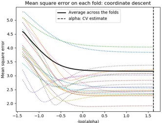
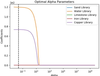
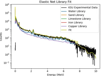
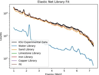
4.1.3 Simulated Example
cross validation, the model was correctly trained to fit only the 3 libraries that contribute to the full spectrum, while providing a zero contribution for the iron and copper libraries. Figures 4-2 thru 4-7 demonstrate how the tuning parameters select the best model and the final fits for LASSO and Elastic Net.
Figure 4-2: Cross validation normalization parameter selection for LASSO
Figure 4-4: LASSO salt water simulation fit
Figure 4-6: Elastic Net model selection by changing normalization parameter
When the normalization parameter is increased, the penalty for each term becomes
greater, allowing the shrinkage and removal of parameters. The MSE at each alpha parameter is
compared, settling on the best overall fit for the final solution. Without putting the output of the
LASSO and Elastic Net fits into an OLS program for a final fit, table 4-1 displays the relative
error of each method averaged over 10 runs.
Table 4-1: Relative error of the two methods Relative Error
Elastic Net LASSO
Water 5.01% 0.07%
Na 2.95% 1.32%
Cl 7.95% 3.65%
4.2 Methods and Improvements
4.2.1 Full Procedure
Before any data analysis can take place, a variety of preprocessing and post processing of data is necessary (Fig. 4-8). Experimental and simulated data are generated at Kansas State and North Carolina State, respectively. The experimental data is processed and separated into counts per channel text files for each detector type, as well as binary files with time dependent data. The detector data is converted into energy bins using calibration sources for empirical FWHM calculations.
The simulated data is generated using MCNP 6.1 using the F8 tally. The nonlinear
response in the Gaussian broadening detector response function is addressed, resulting in a final
Each library is added to a single file and used to train the fitting model. A 10-fold cross
validation process helps reduce the overall bias in model selection. For the test/train split, 90%
of the data is used each time for training, while 10% of the data is held out to test the model.
LASSO and Elastic Net are applied to select the best model that reduces a loss function (MSE).
Once the final solution is reached, the output from LASSO and Elastic Net are used as initial
guesses in an ordinary least squares fitting using CEARLLS.
Figure 4-8: Full procedure
4.2.2 Early Lessons Learned
Figure 4-9: Pure water first fit
To test this theory, a library response for activated Sodium and Iodine are added to the fitting libraries (Fig. 4-10). Although this did improve the overall fit, it did not completely resolve the discrepancies.
To completely understand the nature of the activated (delayed) response, the time
dependent D-T data is necessary. The primary advantage of using a PNG is the ability to read
signatures that are prompt and delayed by the response times. The PNG is triggered using a
firing sequence from the generator and a pulse of neutrons is emitted. After the pulse, there is a
window of time before the next initialization where the neutrons have died off, and the only
remaining signatures are from delayed activation (Figs. 4-11, 4-12).
Figure 4-12: Time dependent format distributed by Kansas State University
4.3 Kansas State Experimental Results
Five separate trials were conducted to provide an experimental basis for this investigation. A water, sand, sand with water, limestone, and limestone with water trial were conducted to provide a broad range of materials and conditions to simulate, fit, and compare to methods currently implemented in the oil well logging industry. Using the post run background measurements, the delayed response is extracted and removed from the final response. The gaussian broadening parameters used for each of these trials was extracted by the method described in section 2.3 as
𝐹𝑊𝐻𝑀 0.031 ∗ 𝐸 . (4.2)
4.3.1 Water Trial
The first trial was conducted using tap water. The channel to energy conversion was accomplished by identifying the peak centroids in the sample and adjusting by
𝐸𝑛𝑒𝑟𝑔𝑦 𝑀𝑒𝑉 .01 .005 ∗ 𝑐ℎ𝑎𝑛𝑛𝑒𝑙 2𝑒 ∗ 𝑐ℎ𝑎𝑛𝑛𝑒𝑙 (4.3)
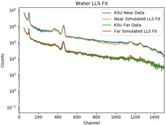
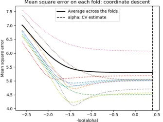
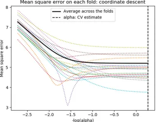
The cross-validation curve (figs. 4-13, 4-17, 4-21, 4-25) demonstrates the process by which the normalization parameter is selected by LASSO and Elastic Net for the near and far detectors. The optimum normalization parameter is presented on the regularization path (figs. 4-14, 4-18, 4-22, 4-26) tracking the coefficients for each library as the normalization parameter changes. The output from the LASSO and Elastic Net codes are presented in figures 4-15, 4-19, 4-23, and 4-27 using only channels 200 thru 1500. The remaining figures provide the full fit using the coefficients determined using the truncated dataset.
Figure 4-14: LASSO model selection coefficients by changing the normalization parameter for the near detector water trial
Figure 4-16: LASSO full fit for the near detector water trial
Figure 4-18: Elastic Net model selection coefficients by changing the normalization parameter for the near detector water trial
Figure 4-20: Elastic Net full fit for the near detector water trial
Figure 4-22: LASSO model selection coefficients by changing the normalization parameter for the far detector water trial
Figure 4-24: LASSO full fit for the far detector water trial
Figure 4-26: Elastic Net model selection coefficients by changing the normalization parameter for the far detector water trial
Figure 4-28: Elastic Net full fit for the far detector water trial
The results show that both LASSO and Elastic Net perform similarly for the near and far detectors. Each correctly identifies the presence of water alone for the near detector, while both misidentifying a copper contribution for the far detectors. Table 4-2 lists the optimal
normalization parameters for each case identified by cross validation. The results for the variable selection process are used as inputs for the final ordinary least squares fitting using the cearlls code. Figures 4-29 and 4-30 display the final fitting and residuals for the near and far detector, respectively. Figure 4-31 shows the near and far final fits together. Tables 4-3, 4-4 provide the chi-squared value, fitting coefficients, and corresponding error for the near and far detectors.
Table 4-2: Optimal normalization parameters for water trial Water Normalization Parameters
Near Detector Far Detector
LASSO 0.464 0.136
Figure 4-29: Linear least squares fit and residual for the near detector water trial
Figure 4-31: Linear least squares fit for near and far detector water trials
Table 4-3: Linear coefficients and error for water near detector Water Linear Least Squares Results – Near Detector
Chi-Squared = 99.3 Coefficients Error
Water 322.6 .051
Sand NA NA
Limestone NA NA
Iron NA NA
Table 4-4: Linear coefficients and error for water far detector Water Linear Least Squares Results – Far Detector
Chi-Squared = 13.3 Coefficients Error
Water 301.9 .12
Sand NA NA
Limestone NA NA
Iron NA NA
Copper NA NA
4.3.2 Sand Trial
The next trial conducted involved pure sand. No chemical or other analysis was performed on the material, so it is assumed that the makeup is SiO2. The channel to energy conversion was
accomplished by identifying the peak centroids in the sample and adjusting by
𝐸𝑛𝑒𝑟𝑔𝑦 𝑀𝑒𝑉 .051 .00511 ∗ 𝑐ℎ𝑎𝑛𝑛𝑒𝑙 1𝑒 ∗ 𝑐ℎ𝑎𝑛𝑛𝑒𝑙 (4.4)
Figure 4-32: Cross validation normalization parameter selection for the LASSO near detector sand trial
Figure 4-34: LASSO fit for the near detector sand trial
Figure 4-36: Cross validation normalization parameter selection for the Elastic Net near detector sand trial
Figure 4-38: Elastic Net fit for the near detector sand trial
Figure 4-40: Cross validation normalization parameter selection for the LASSO far detector sand trial
Figure 4-42: LASSO fit for the far detector sand trial
Figure 4-44: Cross validation normalization parameter selection for the Elastic Net far detector sand trial
Figure 4-46: Elastic Net fit for the far detector sand trial
The results show that both LASSO and Elastic Net recognize the presence of both sand and water in the near detector, while also detecting iron in the far detector. The detection of water was attributed by the Kansas State University researchers as high humidity from running the test in the summer months, as well as not fully evacuating the test chamber of water before the next test. Table 4-5 lists the optimal normalization parameters for each case identified by cross validation. The results for the variable selection process are used as inputs for the final ordinary least squares fitting using the cearlls code. Figures 4-48 and 4-49 display the final fitting and residuals for the near and far detector, respectively. Figure 4-50 shows the near and far final fits together. Tables 4-6, 4-7 provide the chi-squared value, fitting coefficients, and corresponding error.
Table 4-5: Optimal normalization parameters for sand trial Sand Normalization Parameters
Near Detector Far Detector
LASSO 0.396 1.050
Elastic Net 0.526 0.060
Figure 4-49: Linear least squares fit and residual for the far detector sand trial
Table 4-6: Linear coefficients and error for sand near detector Water Linear Least Squares Results – Near Detector
Chi-Squared = 88.4 Coefficients Error
Water 79.94 1.10
Sand 437.37 0.13
Limestone NA NA
Iron NA NA
Copper NA NA
Table 4-7: Linear coefficients and error for sand far detector Water Linear Least Squares Results – Far Detector
Chi-Squared = 27.6 Coefficients Error
Water 203.90 0.90
Sand 210.55 0.49
Limestone NA NA
Iron NA NA
Copper NA NA
4.3.3 Sand with Water Trial
The next trial conducted involved sand with added water. No chemical or other analysis was performed on the material, so it is assumed that the makeup is SiO2. The channel to energy
conversion was accomplished by identifying the peak centroids in the sample and adjusting by
𝐸𝑛𝑒𝑟𝑔𝑦 𝑀𝑒𝑉 .051 .00511 ∗ 𝑐ℎ𝑎𝑛𝑛𝑒𝑙 1𝑒 ∗ 𝑐ℎ𝑎𝑛𝑛𝑒𝑙 (4.5)
Figure 4-51: Cross validation normalization parameter selection for the LASSO near detector sand and water trial
Figure 4-53: LASSO fit for the near detector sand and water trial
Figure 4-55: Cross validation normalization parameter selection for the Elastic Net near detector sand and water trial
Figure 4-57: Elastic Net fit for the near detector sand and water trial
Figure 4-59: Cross validation normalization parameter selection for the LASSO far detector sand and water trial
Figure 4-61: LASSO fit for the far detector sand and water trial
Figure 4-63: Cross validation normalization parameter selection for the Elastic Net far detector sand and water trial
Figure 4-65: Elastic Net fit for the far detector sand and water trial
The results show that both LASSO and Elastic Net recognize the presence of both sand and water in the near and far detectors. 3 of the 4 tests also include small amounts of iron or copper. Table 4-8 lists the optimal normalization parameters for each case identified by cross validation. The results for the variable selection process are used as inputs for the final ordinary least
squares fitting using the cearlls code. Figures 4-67 and 4-68 display the final fitting and
residuals for the near and far detector, respectively. Figure 4-69 shows the near and far final fits together. Tables 4-9, 4-10 provide the chi-squared value, fitting coefficients, and corresponding error.
Table 4-8: Optimal normalization parameters for sand and water trial Sand and Water Normalization Parameters
Near Detector Far Detector
LASSO 2.495 0.972
Elastic Net 4.385 1.561
Figure 4-68: Linear least squares fit and residual for the far detector sand and water trial