ABSTRACT
HOLM, KATHLEEN JENNIFER. Comparison of Optimal Design Methods in Inverse Problems. (Under the direction of H.T. Banks.)
This project was initiated with an investigation by Banks et al [6] into the use of traditional and generalized sensitivity functions for experimental design. The authors developed tools for finding the best duration of the data ([0, T]), as well as the regions of importance for collecting data based on information from the sensitivity functions. These investigations led to the proposal of a new optimal design method. This work will provide a necessary testing of this new optimal design method with a comparison to more established optimal design methods.
Typical optimal design methods for inverse or parameter estimation problems are designed to choose optimal sampling distributions through minimization of a specific cost function related to the resulting error in parameter estimates. It is hoped that the inverse problem will produce parameter estimates with increased accuracy using data collected according to the optimal sampling distribution. Motivation of the optimal design cost functionals is presented, drawing from linear algebra, geometry and statistics. We formulate the classical optimal design problem in the context of general optimization problems over distributions of sampling times. We present a new Prohorov metric based theoretical framework that permits one to treat succinctly and rigorously any optimal design criteria based on the Fisher Information Matrix (FIM). A fundamental approximation theory is also included in this framework. A new optimal design,
SE-optimal design (standard erroroptimal design), is then introduced in the context of this framework. We compare this new design criteria with the more traditional D-optimal and
E-optimal designs. The optimal sampling distributions from each design are used to compute and compare parameter estimates and standard errors. Given an optimal mesh, the standard errors for parameters are computed using asymptotic theory or bootstrapping. We use three examples to illustrate ideas: the Verhulst-Pearl logistic population model [8], the standard harmonic oscillator model [8] and a popular glucose regulation model [11, 17, 32]. A Monte Carlo analysis provides a comparison of the optimal design methods over a broad spectrum of simulated data sets. We present an overview of modeling autocorrelated data and formulate the inverse problem for the estimation of model and variance parameters. The optimal design methods are compared in the context of autocorrelated data. The consequences of making an incorrect assumption about the independence of the data is investigated for the optimal design time points.
© Copyright 2011 by Kathleen Jennifer Holm
Comparison of Optimal Design Methods in Inverse Problems
by
Kathleen Jennifer Holm
A dissertation submitted to the Graduate Faculty of North Carolina State University
in partial fulfillment of the requirements for the Degree of
Doctor of Philosophy
Biomathematics
Raleigh, North Carolina 2011
APPROVED BY:
Marie Davidian Ralph Smith
Hien Tran H.T. Banks
DEDICATION
BIOGRAPHY
ACKNOWLEDGEMENTS
I am very fortunate for the education I have received from NCSU as a biomath graduate student. Many professors trusted in my abilities and challenged me. Members of the faculty and staff at this university provided me with resources to achieve my goals as a graduate student.
I especially want to express my gratitude to my advisor Dr. Tom Banks. He provided me with guidance both professionally and personally. He also provided me with many opportunities for professional development for which I am grateful. I will always remember the joy he obtained from working with students, his curiosity and enthusiasm for research, and his animated story-telling. I feel honored to be a member of his mathematical family. Dr. Banks and Susie warmly opened their home to graduate students on countless occasions. I greatly appreciate their kindness.
I would also like to thank my thesis committee, Drs. Marie Davidian, Ralph Smith, and Hien Tran, for their advice and guidance in the creation and editing of this dissertation. I am grateful to the professors and graduate students who have collaborated with me on various parts of this dissertation. In particular, I want to thank Franz Kappel, Ariel Cintron-Arias, Danielle Robbins, and Alice Matone.
Through my graduate education I have made many valuable friendships. Many of my math graduate student friends from the University of Arizona helped make my transition to NC State easier including Mia Osorio-Reich, Dan Reich, Serina Diniega, Matej Boguszak, and Suz Ward. I especially appreciate the friendships I have with fellow graduate students at NCSU. Thanks to Ben Wells for all the hiking-adventures and long bike rides. In our mathematical family, Danielle Robbins is my sister. We have experienced so much together. Chad Brown has truly supported me in my final steps of graduate school. In addition, I am grateful to the friendships and bruises provided to me by the Carolina Rollergirls. Roller derby really has been the best graduate school stress-reliever.
TABLE OF CONTENTS
List of Tables . . . vii
List of Figures . . . .xiv
Chapter 1 Introduction . . . 1
Chapter 2 Motivation for Optimal Design Methods . . . 3
2.1 Introduction . . . 3
2.2 Properties of the Fisher information matrix . . . 5
2.3 Relation to Confidence Ellipsoid . . . 8
2.3.1 The Effect of Covariance on the Confidence Ellipsoid . . . 9
2.4 D-optimal . . . 10
2.5 E-optimal . . . 11
2.6 SE-optimal . . . 12
2.7 Discussion . . . 12
Chapter 3 Optimal Design Formulations . . . 14
3.1 Theoretical Summary . . . 16
3.2 Constrained Optimization and Implementations . . . 18
Chapter 4 Inverse Problem and Standard Error Methodology . . . 23
4.1 Standard Error Methodology for Constant Variance Data . . . 23
4.1.1 Asymptotic Theory for Computing Standard Errors . . . 24
4.1.2 Monte Carlo Method for Asymptotic Standard Errors . . . 25
4.1.3 The Bootstrapping Method . . . 26
4.2 Standard Error Methodology for a Vector System . . . 27
4.2.1 Asymptotic Theory for Computing Standard Errors for a Vector System . 28 4.2.2 The Bootstrap Method for a Vector System . . . 29
4.3 Standard Error Methodology for Non-constant Variance Data . . . 30
4.3.1 Asymptotic Theory for Computing Standard Error for Non-Constant Variance Data . . . 31
4.3.2 Bootstrapping Algorithm for Computing Standard Error for Non-constant Variance Data . . . 32
4.4 Choosing the Correct Statistical Model: Constant vs Non-constant Variance . . . 33
4.5 Discussion of Asymptotic Theory vs Bootstrapping . . . 34
Chapter 5 Optimal Design Comparison for Three Examples. . . 35
5.1 The Logistic Growth Example . . . 35
5.1.1 Logistic Model . . . 35
5.1.2 Logistic Results . . . 36
5.1.3 Discussion of Logistic Results . . . 36
5.2.1 Results for the Oscillator Model . . . 42
5.2.2 Discussion for the Oscillator Model . . . 49
5.2.3 Results for the Oscillator Model - with the Inverse Problem . . . 49
5.2.4 Discussion of Oscillator Results with the Inverse Problem . . . 50
5.3 A Simple Glucose Regulation Model . . . 58
5.3.1 Model . . . 58
5.3.2 Results for the Glucose Regulation Model . . . 62
5.3.3 Discussion for the Glucose Regulation Model . . . 63
5.3.4 Result for the Glucose Regulation Model with the Inverse Problem . . . . 65
5.3.5 Discussion for the Glucose Regulation Model with the Inverse Problem . . 66
5.4 Conclusions . . . 75
Chapter 6 Monte Carlo Analysis . . . 77
6.1 Monte Carlo Methodology . . . 77
6.2 Logistic Results . . . 78
6.2.1 Discussion of Logistic Monte Carlo Results . . . 81
6.3 Harmonic Oscillator Results . . . 90
6.3.1 Discussion of Harmonic Oscillator Monte Carlo Results . . . 112
Chapter 7 Autocorrelated Data with Applications to Optimal Design Methods114 7.1 Introduction . . . 114
7.2 Detection . . . 114
7.3 Autocorrelation Models . . . 116
7.4 Estimation of Parameters in Nonlinear Mathematical Models using Statistical Models with Autocorrelation . . . 118
7.5 Application to Optimal Design Methods . . . 122
7.5.1 Methodology for the Comparison of Optimal Design Methods with Auto-correlation . . . 122
7.5.2 Results of Optimal Design Methods with Autocorrelation . . . 123
7.5.3 Discussion of Optimal Design Methods with Autocorrelation . . . 124
7.6 Using the Incorrect Assumptions on the Correlation in the Errors . . . 128
7.6.1 Results of using the Incorrect Assumptions on the Correlation in the Errors129 7.6.2 Discussion of using the Incorrect Assumption on the Correlation in the Errors . . . 129
7.6.3 The Effect of the Assumptions made within the Optimal Design methods about Correlation in the Errors. . . 138
7.7 Conclusions . . . 141
Chapter 8 Concluding Remarks . . . .143
8.1 Research Conclusions . . . 143
8.2 Future Work . . . 145
LIST OF TABLES
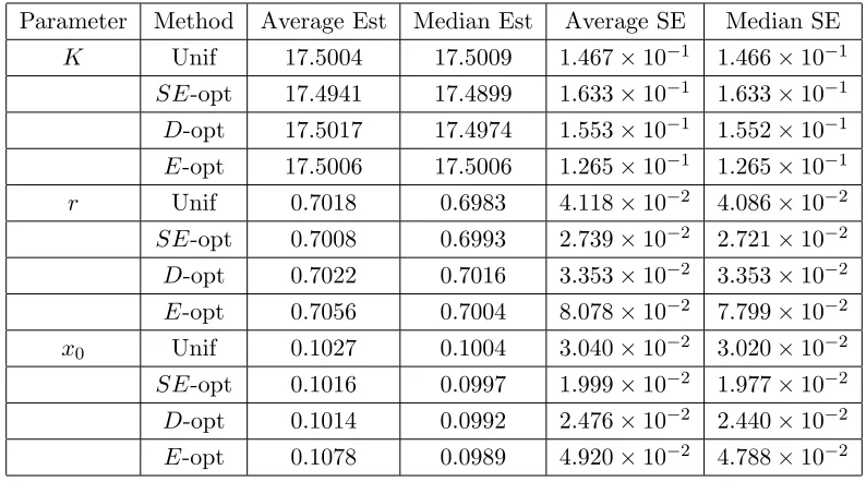
Table 5.1 Average and Median estimates and standard errors using SolvOpt, N = 10, M = 1000, and θ0 = (17.5,0.7,0.1). Optimization with constraint
implementation (C2). . . 37 Table 5.2 Average and Median estimates and standard errors using SolvOpt, N =
15, M = 1000, and θ0 = (17.5,0.7,0.1). Optimization with constraint
implementation (C2). . . 37 Table 5.3 Approximate asymptotic standard errors from the asymptotic theory (4.5)
resulting from different optimal design methods for θ0 = (C, K, x1, x2),
optimization with constraint implementation (C1). . . 44 Table 5.4 Approximate asymptotic standard errors from the asymptotic theory (4.5)
resulting from different optimal design methods for θ0 = (C, K, x1, x2),
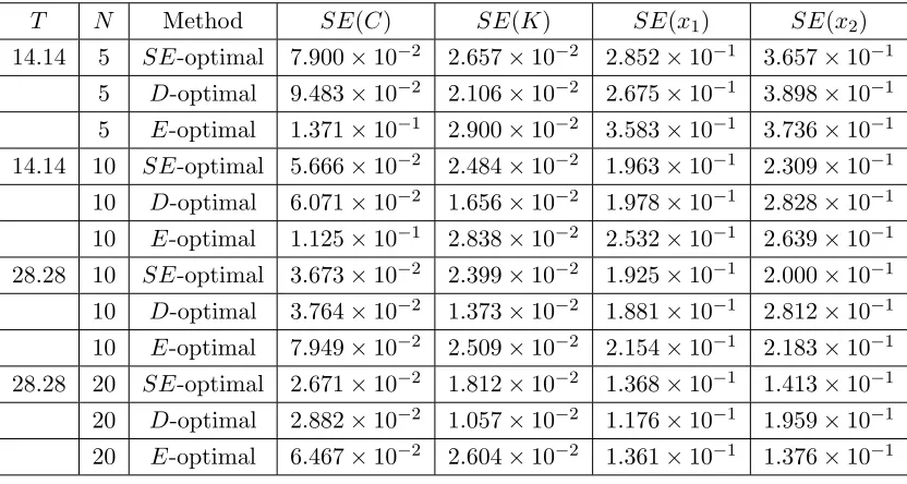
optimization with constraint implementation (C2). . . 44 Table 5.5 Approximate asymptotic standard errors from the asymptotic theory (4.5)
resulting from different optimal design methods for θ0 = (C, K, x1, x2),
optimization with constraint implementation (C3). . . 47 Table 5.6 Approximate asymptotic standard errors from the asymptotic theory (4.5)
resulting from different optimal design methods for θ0 = (C, K, x1, x2),
optimization with constraint implementation (C4). . . 47 Table 5.7 Estimates and standard errors from the asymptotic theory (4.6) resulting
from different optimal design methods (as well as for the uniform mesh) for θ0 = (C, K) = (0.1,0.2) and N = 15, optimization with constraint
implementation (C1). . . 51 Table 5.8 Estimates and standard errors from the bootstrap method (4.9) resulting
from different optimal design methods (as well as for the uniform mesh) for
θ0 = (C, K) = (0.1,0.2),M = 1000 bootstraps andN = 15, optimization
with constraint implementation (C1). . . 51 Table 5.9 Estimates and standard errors from the asymptotic theory (4.6) resulting
from different optimal design methods (as well as for the uniform mesh) for θ0 = (C, K) = (0.1,0.2) and N = 15, optimization with constraint
implementation (C2). . . 52 Table 5.10 Estimates and standard errors from the bootstrap method (4.9) resulting
from different optimal design methods (as well as for the uniform mesh) for
θ0 = (C, K) = (0.1,0.2),M = 1000 bootstraps andN = 15, optimization
with constraint implementation (C2). . . 53 Table 5.11 Estimates and standard errors from the asymptotic theory (4.6) resulting
from different optimal design methods (as well as for the uniform mesh) for θ0 = (C, K) = (0.1,0.2) and N = 15, optimization with constraint
Table 5.12 Estimates and standard errors from the bootstrap method (4.9) resulting from different optimal design methods (as well as for the uniform mesh) for
θ0 = (C, K) = (0.1,0.2),M = 1000 bootstraps andN = 15, optimization
with constraint implementation (C3). . . 54 Table 5.13 Estimates and standard errors from the asymptotic theory (4.6) resulting
from different optimal design methods (as well as for the uniform mesh) for θ0 = (C, K) = (0.1,0.2) and N = 15, optimization with constraint
implementation (C4). . . 55 Table 5.14 Estimates and standard errors from the bootstrap method (4.9) resulting
from different optimal design methods (as well as for the uniform mesh) for
θ0 = (C, K) = (0.1,0.2),M = 1000 bootstraps andN = 15, optimization
with constraint implementation (C4). . . 56 Table 5.15 Description of model parameters and typical values. . . 59 Table 5.16 Approximate asymptotic standard errors from the asymptotic theory (4.5)
resulting from different optimal design methods for θ0 = (p1, p2, p3, p4),
optimization, using SolvOpt, with constraint implementation (C1). . . 63 Table 5.17 Approximate asymptotic standard errors from the asymptotic theory (4.5)
resulting from different optimal design methods for θ0 = (p1, p2, p3, p4),
optimization, using SolvOpt, with constraint implementation (C2). . . 64 Table 5.18 Approximate asymptotic standard errors from the asymptotic theory (4.5)
resulting from different optimal design methods for θ0 = (p1, p2, p3, p4),
optimization, using SolvOpt, with constraint implementation (C3). . . 65 Table 5.19 Approximate asymptotic standard errors from the asymptotic theory (4.5)
resulting from different optimal design methods for θ0 = (p1, p2, p3, p4),
optimization, using SolvOpt, with constraint implementation (C4). . . 66 Table 5.20 Estimates, standard errors, and covariances between parameters from the
asymptotic theory (4.6) resulting from different optimal design methods (as well as for the uniform mesh) for θ0 = (p1, p2, p3, p4) = (2.6×10−2,2.5×
10−2,1.25×10−5,4.1×10−3) and N = 30, optimization, using fmincon, with constraint implementation (C1). . . 67 Table 5.21 Estimates, standard errors, and covariances between parameters from the
bootstrap method (4.9) resulting from different optimal design methods (as well as for the uniform mesh) for θ0 = (p1, p2, p3, p4) = (2.6×10−2,2.5×
10−2,1.25×10−5,4.1×10−3),M = 1000 bootstraps andN = 30, optimiza-tion, using fmincon, with constraint implementation (C1). . . 68 Table 5.22 Estimates, standard errors, and covariances between parameters from the
asymptotic theory (4.6) resulting from different optimal design methods (as well as for the uniform mesh) for θ0 = (p1, p2, p3, p4) = (2.6×10−2,2.5×
10−2,1.25×10−5,4.1×10−3) and N = 30, optimization, using fmincon,
Table 5.23 Estimates, standard errors, and covariances between parameters from the bootstrap method (4.9) resulting from different optimal design methods (as well as for the uniform mesh) for θ0 = (p1, p2, p3, p4) = (2.6×10−2,2.5×
10−2,1.25×10−5,4.1×10−3),M = 1000 bootstraps andN = 30, optimiza-tion, using fmincon, with constraint implementation (C2). . . 70 Table 5.24 Estimates, standard errors, and covariances between parameters from the
asymptotic theory (4.6) resulting from different optimal design methods (as well as for the uniform mesh) for θ0 = (p1, p2, p3, p4) = (2.6×10−2,2.5×
10−2,1.25×10−5,4.1×10−3) and N = 30, optimization, using fmincon, with constraint implementation (C3). . . 71 Table 5.25 Estimates, standard errors, and covariances between parameters from the
bootstrap method (4.9) resulting from different optimal design methods (as well as for the uniform mesh) for θ0 = (p1, p2, p3, p4) = (2.6×10−2,2.5×
10−2,1.25×10−5,4.1×10−3),M = 1000 bootstraps andN = 30, optimiza-tion, using fmincon, with constraint implementation (C3). . . 72 Table 5.26 Estimates, standard errors, and covariances between parameters from the
asymptotic theory (4.6) resulting from different optimal design methods (as well as for the uniform mesh) for θ0 = (p1, p2, p3, p4) = (2.6×10−2,2.5×
10−2,1.25×10−5,4.1×10−3) and N = 30, optimization, using fmincon, with constraint implementation (C4). . . 73 Table 5.27 Estimates, standard errors, and covariances between parameters from the
bootstrap method (4.9) resulting from different optimal design methods (as well as for the uniform mesh) for θ0 = (p1, p2, p3, p4) = (2.6×10−2,2.5×
10−2,1.25×10−5,4.1×10−3),M = 1000 bootstraps andN = 30, optimiza-tion, using fmincon, with constraint implementation (C4). . . 74 Table 6.1 Average estimates (θAvg) with their standard deviations (θSD) fromM =
1000 Monte Carlo trials as well as asymptotic standard errors (SE(θ)). Data was simulated using true valuesθ0 = (17.5,0.7,0.1), N = 10, and 1%
noise (σ20 = 0.01). . . 79 Table 6.2 Average estimates (θAvg) with their standard deviations (θSD) fromM =
1000 Monte Carlo trials as well as asymptotic standard errors (SE(θ)). Data was simulated using true valuesθ0 = (17.5,0.7,0.1), N = 10, and 5%
noise (σ2
0 = 0.05). . . 80
Table 6.3 Average estimates (θAvg) with their standard deviations (θSD) fromM = 1000 Monte Carlo trials as well as asymptotic standard errors (SE(θ)). Data was simulated using true values θ0 = (17.5,0.7,0.1), N = 10, and
10% noise (σ02= 0.10). . . 80 Table 6.4 Percent of Confidence Ellipsoids which contain the true parameter values
(N=10). . . 84 Table 6.5 Average estimates (θAvg) with their standard deviations (θSD) fromM =
1000 Monte Carlo trials as well as asymptotic standard errors (SE(θ)). Data was simulated using true valuesθ0 = (17.5,0.7,0.1), N = 15, and 1%
Table 6.6 Average estimates (θAvg) with their standard deviations (θSD) fromM =
1000 Monte Carlo trials as well as asymptotic standard errors (SE(θ)). Data was simulated using true valuesθ0 = (17.5,0.7,0.1), N = 15, and 5%
noise (σ20 = 0.05). . . 85 Table 6.7 Average estimates (θAvg) with their standard deviations (θSD) fromM =
1000 Monte Carlo trials as well as asymptotic standard errors (SE(θ)). Data was simulated using true values θ0 = (17.5,0.7,0.1), N = 15, and
10% noise (σ02= 0.10). . . 85 Table 6.8 Percent of Confidence Ellipsoids which contain the true parameter values
(N=15). . . 89 Table 6.9 Average estimates (θAvg) with their standard deviations (θSD) fromM =
1000 Monte Carlo trials as well as asymptotic standard errors (SE(θ)). Data was simulated using true values θ0 = (C, K) = (0.1,0.2), fixed
parameter values (x1, x2) = (−1,0.5), and noise levelσ20 = 0.01. Simulated
data corresponds to optimal design points using N = 15, T = 14.14 and
T = 28.28, and constraint implementation (C1). . . 92 Table 6.10 Average estimates (θAvg) with their standard deviations (θSD) fromM =
1000 Monte Carlo trials as well as asymptotic standard errors (SE(θ)). Data was simulated using true values θ0 = (C, K) = (0.1,0.2), fixed
parameter values (x1, x2) = (−1,0.5), and noise levelσ20 = 0.05. Simulated
data corresponds to optimal design points using N = 15, T = 14.14 and
T = 28.28, and constraint implementation (C1). . . 93 Table 6.11 Average estimates (θAvg) with their standard deviations (θSD) fromM =
1000 Monte Carlo trials as well as asymptotic standard errors (SE(θ)). Data was simulated using true values θ0 = (C, K) = (0.1,0.2), fixed
parameter values (x1, x2) = (−1,0.5), and noise levelσ20 = 0.10. Simulated
data corresponds to optimal design points using N = 15, T = 14.14 and
T = 28.28, and constraint implementation (C1). . . 94 Table 6.12 Percent of Confidence Ellipsoids which contain the true parameter values
(T = 14.14, constraint implementation (C1)). . . 94 Table 6.13 Percent of Confidence Ellipsoids which contain the true parameter values
(T = 28.28, constraint implementation (C1)). . . 96 Table 6.14 Average estimates (θAvg) with their standard deviations (θSD) fromM =
1000 Monte Carlo trials as well as asymptotic standard errors (SE(θ)). Data was simulated using true values θ0 = (C, K) = (0.1,0.2), fixed
parameter values (x1, x2) = (−1,0.5), and noise levelσ20 = 0.01. Simulated
data corresponds to optimal design points using N = 15, T = 14.14 and
T = 28.28 and constraint implementation (C2). . . 96 Table 6.15 Average estimates (θAvg) with their standard deviations (θSD) fromM =
1000 Monte Carlo trials as well as asymptotic standard errors (SE(θ)). Data was simulated using true values θ0 = (C, K) = (0.1,0.2), fixed
parameter values (x1, x2) = (−1,0.5), and noise levelσ20 = 0.05. Simulated
data corresponds to optimal design points using N = 15, T = 14.14 and
Table 6.16 Average estimates (θAvg) with their standard deviations (θSD) fromM =
1000 Monte Carlo trials as well as asymptotic standard errors (SE(θ)). Data was simulated using true values θ0 = (C, K) = (0.1,0.2), fixed
parameter values (x1, x2) = (−1,0.5), and noise levelσ20 = 0.10. Simulated
data corresponds to optimal design points using N = 15, T = 14.14 and
T = 28.28, and constraint implementation (C2). . . 99 Table 6.17 Percent of Confidence Ellipsoids which contain the true parameter values
(T = 14.14, constraint implementation (C2)). . . 99 Table 6.18 Percent of Confidence Ellipsoids which contain the true parameter values
(T = 28.28, constraint implementation (C2)). . . 101 Table 6.19 Average estimates (θAvg) with their standard deviations (θSD) fromM =
1000 Monte Carlo trials as well as asymptotic standard errors (SE(θ)). Data was simulated using true values θ0 = (C, K) = (0.1,0.2), fixed
parameter values (x1, x2) = (−1,0.5), and noise levelsσ02= 0.01. Simulated
data corresponds to optimal design points using N = 15, T = 14.14 and
T = 28.28, and constraint implementation (C3). . . 101 Table 6.20 Average estimates (θAvg) with their standard deviations (θSD) fromM =
1000 Monte Carlo trials as well as asymptotic standard errors (SE(θ)). Data was simulated using true values θ0 = (C, K) = (0.1,0.2), fixed
parameter values (x1, x2) = (−1,0.5), and noise levelsσ02= 0.05. Simulated
data corresponds to optimal design points using N = 15, T = 14.14 and
T = 28.28, and constraint implementation (C3). . . 103 Table 6.21 Average estimates (θAvg) with their standard deviations (θSD) fromM =
1000 Monte Carlo trials as well as asymptotic standard errors (SE(θ)). Data was simulated using true values θ0 = (C, K) = (0.1,0.2), fixed
parameter values (x1, x2) = (−1,0.5), and noise levelsσ02= 0.10. Simulated
data corresponds to optimal design points using N = 15, T = 14.14 and
T = 28.28, and constraint implementation (C3). . . 104 Table 6.22 Percent of Confidence Ellipsoids which contain the true parameter values
(T = 14.14, constraint implementation (C3)). . . 105 Table 6.23 Percent of Confidence Ellipsoids which contain the true parameter values
(T = 28.28, constraint implementation (C3)). . . 105 Table 6.24 Average estimates (θAvg) with their standard deviations (θSD) fromM =
1000 Monte Carlo trials as well as asymptotic standard errors (SE(θ)). Data was simulated using true values θ0 = (C, K) = (0.1,0.2), fixed
parameter values (x1, x2) = (−1,0.5), and noise levelσ20 = 0.01. Simulated
data corresponds to optimal design points using N = 15, T = 14.14 and
T = 28.28, and constraint implementation (C4). . . 108 Table 6.25 Average estimates (θAvg) with their standard deviations (θSD) fromM =
1000 Monte Carlo trials as well as asymptotic standard errors (SE(θ)). Data was simulated using true values θ0 = (C, K) = (0.1,0.2), fixed
parameter values (x1, x2) = (−1,0.5), and noise levelσ20 = 0.05. Simulated
data corresponds to optimal design points using N = 15, T = 14.14 and
Table 6.26 Average estimates (θAvg) with their standard deviations (θSD) fromM =
1000 Monte Carlo trials as well as asymptotic standard errors (SE(θ)). Data was simulated using true values θ0 = (C, K) = (0.1,0.2), fixed
parameter values (x1, x2) = (−1,0.5), and noise levelσ20 = 0.10. Simulated
data corresponds to optimal design points using N = 15, T = 14.14 and
T = 28.28, and constraint implementation (C4). . . 110 Table 6.27 Percent of Confidence Ellipsoids which contain the true parameter values
(T = 14.14, constraint implementation (C4)). . . 110 Table 6.28 Percent of Confidence Ellipsoids which contain the true parameter values
(T = 28.28, constraint implementation (C4)). . . 112 Table 7.1 Estimates and standard estimates (7.2) from the asymptotic theory resulting
from different optimal design methods (as well as the uniform mesh) for data simulated with θ0 = (K, r, x0) = (17.5,0.7,0.1) and γ0 = (α∗, σ2) =
(0.67,0.10) andN = 15, optimization with constraint implementation (C3). Parameters (K, r, x0, α∗) were estimated using the GEE-1 algorithm. . . . 125
Table 7.2 Average estimates (ˆθAvg) with their standard deviations (ˆθSD) fromM = 1000 Monte Carlo trials. Autocorrelated data corresponding to the optimal time points was simulated using true values (K, r, x0, α∗) = (17.5,0.7,0.1,0.67),
N = 15, and 10% noise (σ20 = 0.10). Parameters (K, r, x0, α∗) were
esti-mated using the GEE-1 algorithm. . . 125 Table 7.3 Average estimates obtained from OLS (ˆθAvg) with their standard deviations
(ˆθSD) and average asymptotic standard errors (7.3) (SE(ˆθ)avg) fromM =
250 Monte Carlo trials. Autocorrelated data corresponding to the optimal time points was simulated using true values (K, r, x0) = (17.5,0.7,0.1),
N = 15, 10% noise (σ02= 0.10), and α∗ = 10−4 autocorrelation. . . 130 Table 7.4 Average estimates obtained from GEE-1 (ˆθAvg) with their standard
devia-tions (ˆθSD) and average asymptotic standard errors (7.2) (SE(ˆθ)avg) from M = 250 Monte Carlo trials. Autocorrelated data corresponding to the opti-mal time points was simulated using true values (K, r, x0) = (17.5,0.7,0.1),
N = 15, 10% noise (σ02= 0.10), and α∗ = 10−4 autocorrelation. . . 130 Table 7.5 Average estimates obtained from OLS (ˆθAvg) with their standard deviations
(ˆθSD) and average asymptotic standard errors (7.3) (SE(ˆθ)avg) fromM =
250 Monte Carlo trials. Autocorrelated data corresponding to the optimal time points was simulated using true values (K, r, x0) = (17.5,0.7,0.1),
N = 15, 10% noise (σ02= 0.10), and α∗ = 0.225 autocorrelation. . . 131 Table 7.6 Average estimates obtained from GEE-1 (ˆθAvg) with their standard
devia-tions (ˆθSD) and average asymptotic standard errors (7.2) (SE(ˆθ)avg) from M = 250 Monte Carlo trials. Autocorrelated data corresponding to the opti-mal time points was simulated using true values (K, r, x0) = (17.5,0.7,0.1),
N = 15, 10% noise (σ2
Table 7.7 Average estimates obtained from OLS (ˆθAvg) with their standard deviations
(ˆθSD) and average asymptotic standard errors (7.3) (SE(ˆθ)avg) fromM =
250 Monte Carlo trials. Autocorrelated data corresponding to the optimal time points was simulated using true values (K, r, x0) = (17.5,0.7,0.1),
N = 15, 10% noise (σ02= 0.10), and α∗ = 0.45 autocorrelation. . . 132 Table 7.8 Average estimates obtained from GEE-1 (ˆθAvg) with their standard
devia-tions (ˆθSD) and average asymptotic standard errors (7.2) (SE(ˆθ)avg) from M = 250 Monte Carlo trials. Autocorrelated data corresponding to the opti-mal time points was simulated using true values (K, r, x0) = (17.5,0.7,0.1),
N = 15, 10% noise (σ2
0 = 0.10), and α∗ = 0.45 autocorrelation. . . 132
Table 7.9 Average estimates obtained from OLS (ˆθAvg) with their standard deviations (ˆθSD) and average asymptotic standard errors (7.3) (SE(ˆθ)avg) fromM =
250 Monte Carlo trials. Autocorrelated data corresponding to the optimal time points was simulated using true values (K, r, x0) = (17.5,0.7,0.1),
N = 15, 10% noise (σ02= 0.10), and α∗ = 0.675 autocorrelation. . . 133 Table 7.10 Average estimates obtained from GEE-1 (ˆθAvg) with their standard
devia-tions (ˆθSD) and average asymptotic standard errors (7.2) (SE(ˆθ)avg) from M = 250 Monte Carlo trials. Autocorrelated data corresponding to the opti-mal time points was simulated using true values (K, r, x0) = (17.5,0.7,0.1),
N = 15, 10% noise (σ02= 0.10), and α∗ = 0.675 autocorrelation. . . 133 Table 7.11 Average estimates obtained from OLS (ˆθAvg) with their standard deviations
(ˆθSD) and average asymptotic standard errors (7.3) (SE(ˆθ)avg) fromM =
250 Monte Carlo trials. Autocorrelated data corresponding to the optimal time points was simulated using true values (K, r, x0) = (17.5,0.7,0.1),
N = 15, 10% noise (σ2
0 = 0.10), and α∗ = 0.9 autocorrelation. . . 134
Table 7.12 Average estimates obtained from GEE-1 (ˆθAvg) with their standard devia-tions (ˆθSD) and average asymptotic standard errors (7.2) (SE(ˆθ)avg) from M = 250 Monte Carlo trials. Autocorrelated data corresponding to the opti-mal time points was simulated using true values (K, r, x0) = (17.5,0.7,0.1),
N = 15, 10% noise (σ02= 0.10), and α∗ = 0.9 autocorrelation. . . 134 Table 7.13 Average estimates obtained from OLS (ˆθAvg) with their standard deviations
(ˆθSD) and average asymptotic standard errors (7.3) (SE(ˆθ)avg) fromM =
250 Monte Carlo trials. Autocorrelated data corresponding to the optimal time points with autocorrelation assumption was simulated using true values (K, r, x0) = (17.5,0.7,0.1), N = 15, 10% noise (σ02 = 0.10), and
α∗ = 0.9 autocorrelation. . . 139 Table 7.14 Average estimates obtained from GEE-1 (ˆθAvg) with their standard
devia-tions (ˆθSD) and average asymptotic standard errors (7.2) (SE(ˆθ)avg) from M = 250 Monte Carlo trials. Autocorrelated data corresponding to the optimal time points with autocorrelation assumption was simulated using true values (K, r, x0) = (17.5,0.7,0.1),N = 15, 10% noise (σ20 = 0.10), and
LIST OF FIGURES
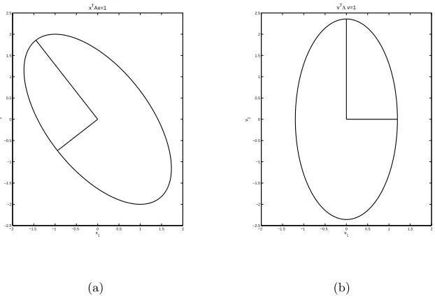
Figure 2.1 Ellipses corresponding to symmetric positive-definite matrices, xTAx= 1 (panel (a)), and linear transformation into orthonormal set of eigenvectors of A: (xTS−1)Λ(Sx) = vTΛv = 1 (panel (b)). Both plots have the same axes bounds, tick marks and dimensions, though plotted in different variables (x: panel (a),v: panel (b)). . . 8 Figure 5.1 The distribution of optimal time points and uniform sampling time points
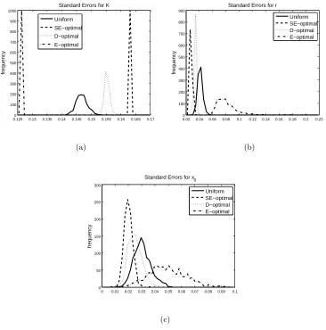
plotted on the logistic curve. Optimal times points obtained using SolvOpt, withN = 10, and the optimal design methodsSE-optimality,D-optimality, and E-optimality. Optimization with constraint implementation (C2). . . 38 Figure 5.2 Using SolvOpt, with N = 10, a comparison of optimal design methods
usingSE-optimality,D-optimality,E-optimality, with a uniform sampling time points in terms ofSEK (panel (a)),SEr(panel (b)), andSEx0 (panel
(c)). Optimization with constraint implementation (C2). . . 39 Figure 5.3 The distribution of optimal time points and uniform sampling time points
plotted on the logistic curve. Optimal times points obtained using SolvOpt, withN = 15, and the optimal design methodsSE-optimality,D-optimality, and E-optimality. Optimization with constraint implementation (C2). . . 40 Figure 5.4 Using SolvOpt, with N = 15, a comparison of optimal design methods
usingSE-optimality,D-optimality,E-optimality, with a uniform sampling time points in terms ofSEK (panel (a)),SEr(panel (b)), andSEx0 (panel
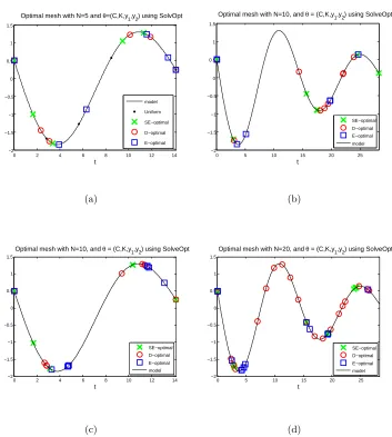
(c)). Optimization with constraint implementation (C2). . . 41 Figure 5.5 Plot of model with optimal time points resulting from different optimal
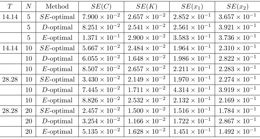
design methods for θ0 = (C, K, x1, x2), with T = 14.14 (one period) for
N = 5 (panel (a)) andN = 10 (panel (c)) andT = 28.28 (two periods) for
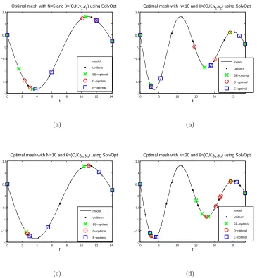
N = 10 (panel (b)) andN = 20 (panel (d)). Optimization with constraint implementation (C1). . . 43 Figure 5.6 Plot of model with optimal time points resulting from different optimal
design methods for θ0 = (C, K, x1, x2), with T = 14.14 (one period) for
N = 5 (panel (a)) andN = 10 (panel (c)) andT = 28.28 (two periods) for
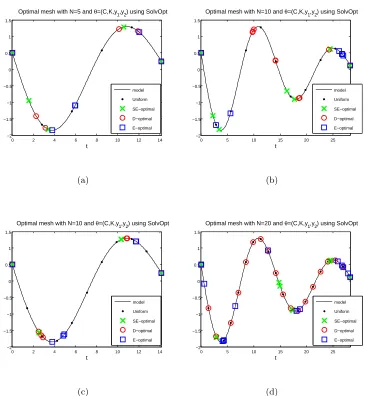
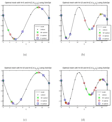
N = 10 (panel (b)) andN = 20 (panel (d)). Optimization with constraint implementation (C2). . . 45 Figure 5.7 Plot of model with optimal time points resulting from different optimal
design methods for θ0 = (C, K, x1, x2), with T = 14.14 (one period) for
N = 5 (panel (a)) andN = 10 (panel (c)) andT = 28.28 (two periods) for
Figure 5.8 Plot of model with optimal time points resulting from different optimal design methods for θ0 = (C, K, x1, x2), with T = 14.14 (one period) for
N = 5 (panel (a)) andN = 10 (panel (c)) andT = 28.28 (two periods) for
N = 10 (panel (b)) andN = 20 (panel (d)). Optimization with constraint implementation (C4). . . 48 Figure 5.9 Plot of model with optimal time points resulting from different optimal
design methods for θ0 = (C, K), N = 15, with T = 14.14 (one period)
(panel (a)) andT = 28.28 (two periods) (panel (b)). Optimization with constraint implementation (C1). . . 50 Figure 5.10 Plot of model with optimal time points resulting from different optimal
design methods for θ0 = (C, K), N = 15, with T = 14.14 (one period)
(panel (a)) andT = 28.28 (two periods) (panel (b)). Optimization with constraint implementation (C2). . . 52 Figure 5.11 Plot of model with optimal time points resulting from different optimal
design methods for θ0 = (C, K), N = 15, with T = 14.14 (one period)
(panel (a)) andT = 28.28 (two periods) (panel (b)). Optimization with constraint implementation (C3). . . 53 Figure 5.12 Plot of model with optimal time points resulting from different optimal
design methods for θ0 = (C, K), N = 15, with T = 14.14 (one period)
(panel (a)) andT = 28.28 (two periods) (panel (b)). Optimization with constraint implementation (C4). . . 55 Figure 5.13 Plot of model with optimal time points resulting from different optimal
design methods forθ0= (p1, p2, p3, p4), withT = 150 forN = 30. Optimal
time points with the Glucose model in panel (a) and with the Insulin model in panel (b). Optimization, using SolvOpt, with constraint implementation (C1). . . 62 Figure 5.14 Plot of model with optimal time points resulting from different optimal
design methods forθ0= (p1, p2, p3, p4), withT = 150 forN = 30. Optimal
time points with the Glucose model in panel (a) and with the Insulin model in panel (b). Optimization, using SolvOpt, with constraint implementation (C2). . . 63 Figure 5.15 Plot of model with optimal time points resulting from different optimal
design methods forθ0= (p1, p2, p3, p4), withT = 150 forN = 30. Optimal
time points with the Glucose model in panel (a) and with the Insulin model in panel (b). Optimization, using SolvOpt, with constraint implementation (C3). . . 64 Figure 5.16 Plot of model with optimal time points resulting from different optimal
design methods forθ0= (p1, p2, p3, p4), withT = 150 forN = 30. Optimal
Figure 6.1 A generic example of 95% Confidence Ellipsoids (from M = 30 simulated data sets, estimating p = 2 parameters), where the true value is given by the star, confidence ellipsoids containing the true value are gray, and confidence ellipsoids not containing the true value are black. . . 79 Figure 6.2 Histograms of parameter estimates (Kb in panel (a), ˆr in panel (b), ˆx0 in
panel (c)) resulting from Monte Carlo simulation withM = 1000. Different histograms within each subfigure represent results from different optimal design methods as well as from the uniform mesh. Simulated data was generated with N = 10 and 1% noise (σ20 = 0.01). . . 81 Figure 6.3 Histograms of parameter estimates (Kb in panel (a), ˆr in panel (b), ˆx0 in
panel (c)) resulting from Monte Carlo simulation withM = 1000. Different histograms within each subfigure represent results from different optimal design methods as well as from the uniform mesh. Simulated data was generated with N = 10 and 5% noise (σ20 = 0.05). . . 82 Figure 6.4 Histograms of parameter estimates (Kb in panel (a), ˆr in panel (b), ˆx0 in
panel (c)) resulting from Monte Carlo simulation withM = 1000. Different histograms within each subfigure represent results from different optimal design methods as well as from the uniform mesh. Simulated data was generated with N = 10 and 10% noise (σ20 = 0.10). . . 83 Figure 6.5 Histograms of parameter estimates (Kb in panel (a), ˆr in panel (b), ˆx0 in
panel (c)) resulting from Monte Carlo simulation withM = 1000. Different histograms within each subfigure represent results from different optimal design methods as well as from the uniform mesh. Simulated data was generated with N = 15 and 1% noise (σ20 = 0.01). . . 86 Figure 6.6 Histograms of parameter estimates (Kb in panel (a), ˆr in panel (b), ˆx0 in
panel (c)) resulting from Monte Carlo simulation withM = 1000. Different histograms within each subfigure represent results from different optimal design methods as well as from the uniform mesh. Simulated data was generated with N = 15 and 5% noise (σ20 = 0.05). . . 87 Figure 6.7 Histograms of parameter estimates (Kb in panel (a), ˆr in panel (b), ˆx0 in
panel (c)) resulting from Monte Carlo simulation withM = 1000. Different histograms within each subfigure represent results from different optimal design methods as well as from the uniform mesh. Simulated data was generated with N = 15 and 10% noise (σ20 = 0.10). . . 88 Figure 6.8 Histograms of parameter estimates (Cb in panels (a),(c),(e), and Kb in
panel (b),(d),(f)) resulting from Monte Carlo simulation. Simulated data was generated with σ02 = 0.01 (top row), σ20 = 0.05 (middle row), and
σ20 = 0.10 (bottom row) (T = 14.14 and constraint implementation (C1)). 91 Figure 6.9 Histograms of parameter estimates (Cb in panels (a),(c),(e), and Kb in
panel (b),(d),(f)) resulting from Monte Carlo simulation. Simulated data was generated with σ02 = 0.01 (top row), σ20 = 0.05 (middle row), and
Figure 6.10 Histograms of parameter estimates (Cb in panels (a),(c),(e), and Kb in panel (b),(d),(f)) resulting from Monte Carlo simulation. Simulated data was generated with σ02 = 0.01 (top row), σ20 = 0.05 (middle row), and
σ20 = 0.10 (bottom row) (T = 14.14 and constraint implementation (C2)). 97 Figure 6.11 Histograms of parameter estimates (Cb in panels (a),(c),(e), and Kb in
panel (b),(d),(f)) resulting from Monte Carlo simulation. Simulated data was generated with σ02 = 0.01 (top row), σ20 = 0.05 (middle row), and
σ20 = 0.10 (bottom row) (T = 28.28 and constraint implementation (C2)). 100 Figure 6.12 Histograms of parameter estimates (Cb in panels (a),(c),(e), and Kb in
panel (b),(d),(f)) resulting from Monte Carlo simulation. Simulated data was generated with σ02 = 0.01 (top row), σ20 = 0.05 (middle row), and
σ20 = 0.10 (bottom row) (T = 14.14 and constraint implementation (C3)). 102 Figure 6.13 Histograms of parameter estimates (Cb in panels (a),(c),(e), and Kb in
panel (b),(d),(f)) resulting from Monte Carlo simulation. Simulated data was generated with σ02 = 0.01 (top row), σ20 = 0.05 (middle row), and
σ2
0 = 0.10 (bottom row) (T = 28.28 and constraint implementation (C3)). 106
Figure 6.14 Histograms of parameter estimates (Cb in panels (a),(c),(e), and Kb in panel (b),(d),(f)) resulting from Monte Carlo simulation. Simulated data was generated with σ02 = 0.01 (top row), σ20 = 0.05 (middle row), and
σ20 = 0.10 (bottom row) (T = 14.14 and constraint implementation (C4)). 107 Figure 6.15 Histograms of parameter estimates (Cb in panels (a),(c),(e), and Kb in
panel (b),(d),(f)) resulting from Monte Carlo simulation. Simulated data was generated with σ02 = 0.01 (top row), σ20 = 0.05 (middle row), and
σ20 = 0.10 (bottom row) (T = 28.28 and constraint implementation (C4)). 111 Figure 7.1 The distribution of optimal time points and uniform sampling time points
plotted on the logistic curve. Optimal times points assuming an exponential autocorrelation model were obtained using SolvOpt, with N = 10 (panel (a)) andN = 15 (panel (b)). . . 124 Figure 7.2 Histograms of parameter estimates (K in panel (a), r in panel (b), x0 in
panel (c), α∗ in panel (d)) resulting from Monte Carlo simulation with M = 1000. Different histograms within each subgure represent results from different optimal design methods as well as from the uniform mesh. Simulated autocorrelated data was generated with N = 15, α∗ = 0.67, 10% noise (σ20 = 0.10), and true parameter values θ0 = (K, r, x0) =
Chapter 1
Introduction
Mathematical models are used to describe dynamics arising from biological, physical and engineering systems. If the parameters in the model are known, the model can be used for simulation, prediction, control design, etc. However, typically one does not have accurate values for the parameters. Instead, one must estimate the parameters using experimental data. The simulation and predictive capabilities of the model depend on the accuracy of the parameter estimates. A major question that experimentalists and inverse problem investigators alike often face is how to best collect the data to enable one to efficiently and accurately estimate model parameters. This is the well-known and widely studied optimal designproblem.
Traditional optimal design methods (D-optimal,E-optimal,c-optimal) [1, 2, 9, 20, 21] use information from the model to find the sampling distribution or mesh for the observation times (and/or locations in spatially distributed problems) that minimizes a design criterion, quite often a function of the Fisher Information Matrix (FIM). Experimental data taken on this optimal mesh is then expected to result in accurate parameter estimates.
A new optimal design,SE-optimal design (standard erroroptimal design), is introduced and compared with the more traditional D-optimal andE-optimal designs. SE-optimal design was first introduced in [6]. The goal ofSE-optimal design is to find the observation times τ ={ti}
that minimize the sum of squared normalized standard errors of the estimated parameters as defined by asymptotic distribution results from statistical theories [5, 7, 15, 30]. D-optimal andE-optimal design methods minimize functions of the covariance in the parameter estimates [2, 9, 21]. D-optimal design finds the mesh that minimizes the volume of the confidence ellipsoid of the asymptotic covariance matrix. E-optimal design minimizes the largest principle axis of the confidence ellipsoid of the asymptotic covariance matrix.
because they offer qualitatively different solutions. The Verhulst-Pearl logistic population model is a very well studied model [6, 7, 8] whose solution is a monotone increasing trajectory with a steady state. The harmonic oscillator model [8], whose solution oscillations which decay over time may provide increased challenges to the optimal design methods. The glucose regulation model [10, 11, 17, 25] is a more complex system of nonlinear differential equations with a vector observation or model output. The glucose regulation model also has a clinical application to the diagnosis of diabetes which could potentially benefit in the information obtained using optimal design methods.
In an effort to provide a reasonably fair comparison, for each optimal design method, standard errors are computed by several methods using the optimal mesh. The optimal design methods are compared based on these standard errors. The goal of this dissertation is not just to test the newer optimal design method,SE-optimal, against the more traditional optimal design methods,
D-optimal and E-optimal. We also hope to motivate the use of optimal design methods in a range of practical applications where experimentalists and modelers have common goals to increase efficiency and accuracy in parameter estimates.
Chapter 2
Motivation for Optimal Design
Methods
2.1
Introduction
Optimal design methods use information from the model to find the sampling distribution or mesh for the observation times (and/or locations in spatially distributed problems) that minimizes a design criterion, quite often a function of the Fisher information matrix (FIM). Experimental data taken on this optimal mesh are then expected to result in accurate parameter estimates.
In this chapter we will give the motivation behind the three optimal design methods we consider in this comparison. First we must briefly introduce the setting in which we will employ these optimal design methods. Underlying our considerations is amathematical model, which may describe some physical, sociological or biological phenomenon, e.g.,
˙
x(t) = g(t, x(t), q),
x(0) = x0, (2.1)
f(t, θ) = C(x(t, θ)), t∈[0, T],
where x(t) ∈ Rn is the vector of state variables of the system, f(t, θ) ∈ Rm is the vector of observable or measurable outputs,q∈Rrare the system parameters,θ= (q, x
0)∈Rp, p=r+n
is the vector of system parameters plus initial conditions x0, while g and C are mappings
R1+n+r→ Rn andRn →Rm, respectively. To consider measures of uncertainty in estimated parameters [5], one also requires a statistical model. Our statistical model is given by the stochastic process
Here E is a noisy random process representing measurement errors and, as usual in statistical formulations [5, 6, 30], θ0 is a hypothesized “true” value of the unknown parameters. Let
σ(t)2= Var(E(t)). We make the following standard assumptions on the random variable E(t)
throughout our analysis in Chapters 5 and 6:
E(E(t)) = 0, t∈[0, T],
Var(E(t)) = σ20, t∈[0, T],
Cov(E(t)E(s)) = σ20δ(t−s), t, s∈[0, T],
where δ(s) = 1 fors= 0 andδ(s) = 0 for s6= 0. A realization of the observation process is given by
y(t) =f(t, θ0) +ε(t), t∈[0, T],
where the measurement error ε(t) is a realization ofE(t). Usually our observed data is discrete,{tj, yj}N
j=1. Optimal design methods seek the sampling
distribution of times,τ ={tj}N
j=1, that will minimize some function of the Fisher information
matrix, F = Σ−1, where Σ is the covariance matrix Σ =σ02χT(θ0)χ(θ0)
−1
,
whereχis theN×p(number of time points: N, and number of parameters: p) sensitivity matrix such that χi,j = ∂f∂θ(tij,θ) fori= 1, . . . , N and j= 1, . . . , p, θ0 is the vector of true parameters,
and σ02 is the true constant variance of the model residuals.
Each optimal design method proposes its own cost functional,J(F). To obtain the optimal design points, τ∗={t∗i},i= 1, . . . , N, one must perform the following minimization.
J(F(τ∗, θ0,)) = min
τ∈T J(F(τ, θ0)),
where T is the set of all time meshes such that 0≤t1 ≤ · · · ≤ti≤ti+1≤ · · · ≤tN ≤T.
2.2
Properties of the Fisher information matrix
The discrete asymptotic Fisher information matrix (FIM) is defined as
F = 1
σ02
χT(θ0)χ(θ0)
.
Note: For any m×n matrixA of (column) rankr, the productATAis a symmetric matrix and its rank is alsor [31]. This implies that if the sensitivity matrix, χ, is not full rank, then the Fisher information matrix will also not be full rank, and therefore not invertible (note: Σ =F−1).
Definition: Positive definite matrix
A p×p real-valued matrix A, is called positive definite if xTAx >0 for all non-zero column vectorsx∈Rp.
Definition: Non-negative definite matrix, or Positive semi-definite
Ap×preal-valued matrixA, is called non-negative definite ifxTAx≥0 for all non-zero column vectorsx∈Rp.
The Fisher information and covariance matrices are symmetric (ΣT = Σ) and non-negative definite. The covariance matrix has variance of the parameters along its diagonal and Var(θ)≥0. Additionally, the elements of the covariance are real-valued. By definition Cov(x, y) = Cov(y, x), making the covariance matrix symmetric.
The following theorems will help us prove properties of the confidence ellipsoid.
Theorem(3.25, [29])
If the p×pmatrix Ais symmetric, then
(i) A is positive definite if and only if the eigenvalues ofA,λi>0 for alli= 1, . . . , p.
(ii) A is non-negative definite if and only ifλi≥0 for alli= 1, . . . , pand λi = 0 for at least one
i.
Theorem(3.11, [29])
If ap×pmatrix is symmetric, then it is possible to construct a set of eigenvectors ofA such that the set is orthonormal.
Theorem
LetA be a symmetric positive definite matrix, and x a vector. Then
xTAx= 1
andλ−
1 2
i define the half lengths of the principle axes, whereλiare the corresponding eigenvalues.
Proof
LetA be a p×p matrix, with eigenvalues λi fori= 1. . . p.
Letxbe a vector in the column space ofA. LetSbe ap×pmatrix that contains the orthonormal set of eigenvectors of A; note that S is an orthonormal matrix (S−1 = ST). Let Λ be the corresponding p×p diagonal matrix that contains the corresponding eigenvalues of A. The spectral decomposition of A is [31]
A=S−1ΛS.
We now have a linear transformation from the column space of Ainto the orthonormal space spanned by the eigenvectors of A
Λ =SAS−1.
The ellipsoid defined by xTAx= 1, where x∈Rp, is often tilted. To show that xTAx= 1 truly
gives rise to an ellipse, we want to rotate the ellipse using a linear transformation such that we can write the ellipsoid in standard form:
x1 r1 2 +. . .+ xp rp 2 = 1,
where xT = (x1, x2, . . . , xp)∈Rp, and{r1, . . . , rp}are the elliptical radii or half lengths of the
principle axes. The transformation into the orthonormal space spanned by the eigenvectors of A will transform xTAx= 1 into standard form. Consider the transformationA =S−1ΛS of
xTAx= 1
xTAx=xTS−1ΛSx=xTSTΛSx= (Sx)TΛSx=vTΛv= 1,
where v:=Sx. Now in thev coordinates - the space spanned by the eigenvectors ofA, we can write the ellipse in standard form, let vT = (v1, . . . , vp)
vTΛv= 1,
[v1, . . . , vp]
λ1 0 · · ·
0 λ2 . ..
. .. ... ...
. . . 0 λp
v1 .. . vp
= 1,
[λ1v1, . . . , λpvp]
v1 .. . vp
λ1v21+. . .+λpvp2= 1, v1 λ− 1 2 1 2 +. . .+ vp λ− 1 2 p 2
= 1.
This orthonormal eigenvector transformation results in an ellipsoid with minor axes lengths equal to λ−
1 2
i , for i= 1. . . p. The axes are aligned with v, the space spanned by the orthogonal
eigenvectors of A. Therefore the original xTAx = 1 gives the equation for an ellipse with
principle axis corresponding to the orthonormal eigenvectors of A with minor axes of length
λ−
1 2
i , fori= 1. . . p, whereλi,i= 1. . . p, are the eigenvalues ofA. Example: Let Abe defined as follows
A= 3 −2
−2 4
!
.
Note thatAis symmetric positive definite. We are interested in the ellipse formed byxTAx= 1.
To demonstrate the theorem above we will plot the ellipse formed by matrix A. We will also show how the spectral decomposition of Awill form an equivalent ellipse rotated into the space spanned by the eigenvectors of A. The spectral decomposition is defined by
A=S−1ΛS.
For this example, the spectral decomposition of A is given by
A= −.7882 −.6154
−.6154 .7882
!
1.4384 0 0 5.5616
!
−.7882 −.6154
−.6154 .7882
!
.
In Fig. 2.1 are the ellipses formed byA and the transformation derived above: vTΛv= 1. The ellipse formed by Ais tilted with axes in the direction of its two eigenvectors (with slopes ≈
1.28, and -0.78). The half lengths of the two axis are the same in both plots and are equal to
λ−
1 2
i ≈(1.4384
−1
2,5.5616−
1
2) = (.8338, .4240). The plot on the right is just a rotation of the plot
−2 −1.5 −1 −0.5 0 0.5 1 1.5 2 −2.5
−2 −1.5 −1 −0.5 0 0.5 1 1.5 2 2.5
x1 x2
xTAx=1
(a)
−2 −1.5 −1 −0.5 0 0.5 1 1.5 2 −2.5
−2 −1.5 −1 −0.5 0 0.5 1 1.5 2 2.5
v1 v2
vTΛ v=1
(b)
Figure 2.1: Ellipses corresponding to symmetric positive-definite matrices,xTAx= 1 (panel (a)), and linear transformation into orthonormal set of eigenvectors ofA: (xTS−1)Λ(Sx) =vTΛv= 1
(panel (b)). Both plots have the same axes bounds, tick marks and dimensions, though plotted in different variables (x: panel (a), v: panel (b)).
2.3
Relation to Confidence Ellipsoid
The confidence ellipsoid is a visualization of the confidence intervals for multiple parameter estimates all in the common parameter space. The confidence ellipsoid is defined as
(θ−θˆ)TFb(θ−θˆ) =m,
where the parameter estimate is ˆθ, the estimated Fisher information matrix isFb=Σb−1, and
m represents the test statistic associated with the confidence level, α, for the 100%(1−α) confidence ellipsoid and the sample size, N. The definition of the specific test statistic requires assumptions about the distribution of the residuals. A common distributional assumption is to take E ∼ N(0, σ02). This assumption results in the 100(1−α)% confidence ellipsoid being defined by [30]
(θ−θˆ)TFb(θ−θˆ) =pFαp,N−p ⇐⇒
(θ−θˆ)T[χT(ˆθ)χ(ˆθ)](θ−θˆ)
pσˆ2 = F
where Fαp,N−p denotes the F-distribution with numerator degrees of freedom pand denominator degrees of freedom (N−p) at theα critical level. Note herem=pFαp,N−p.
The confidence ellipsoid will have principle axes along the eigenvectors ofF inRp, possibly tilted when plotted on the θT = (θ1, . . . , θp) axes. The confidence ellipsoid will be centered at
the parameter estimates, ˆθ. The half axes will be proportional to (due to the constantm) λ−
1 2
i ,
where λi represents the eigenvalues ofF (i= 1. . . p). Note thatλ−
1 2
i = (λ
−1
i )
1
2 = ˜λ
1 2
i , where ˜λi
are the eigenvalues of Σ, assumingF is invertible. As the width of the confidence interval is proportional to the standard error in the estimates, the length of the axes in the confidence ellipsoid are also proportional to the standard error. The 100(1−α)% confidence interval is defined as [5]
ˆ
θ±tN1−−α/p2SE(ˆθ),
where the standard error is given by SE(ˆθi) = √
Σii fori= 1. . . p.
The theorem proved in the previous section holds for symmetric positive definite matrices. The Fisher information matrix is only symmetric non-negative definite. Supposing that the sensitivity matrix is not of full rank, the FIM will also not be full rank, and the FIM matrix may have at least one zero eigenvalue (λi = 0). Then the ellipsoid ofxTF x= 1 will only haves
principle axes, where sis the number of non-zero eigenvalues (s < p), and the ellipsoid will exist ins-dimensional space, Rs.
2.3.1 The Effect of Covariance on the Confidence Ellipsoid
Covariance between parameters is evident in the tilt of the confidence ellipsoid. If there is no covariance between the parameters, the covariance matrix will be diagonal, and the the confidence ellipsoid will be aligned along the standard axes. Positive covariance between parameters will negatively rotate the ellipsoid (in the clockwise direction) proportional to the degree of covariance between the parameters. Negative covariance between parameters will positively rotate the confidence ellipsoid (in the counter-clockwise direction). Whether or not the optimal design methods are taking the covariance between parameters into effect is still under investigation, and is part of our future research.
2.4
D-optimal
Optimal design methods find the optimal sampling distribution that minimizes some function of the FIM. The cost functional thatD-optimal minimizes is
J(F) = det(F−1).
We will show how minimizing this cost functional is equivalent to minimizing the volume of the confidence ellipsoid.
Let λi fori= 1, ..., p represent the eigenvalues of the matrixA. Then the following holds [31]:
detA=
p
Y
i=1
λi.
Note that this result does not place any requirements on the matrix A.
Consider the ellipsoid with axes’ half lengths equal to r1, . . . , rp. The volume of this ellipsoid
is proportional to the product of the the half lengths
volume(ellipsoid) =C p
Y
i=1
ri,
where C depends on p (e.g. C = π for p = 2, C = 4π/3 for p = 3, C = π2/2 for p = 4,
C= 8π2/15 for p= 5, etc.).
Now let us consider the volume of the confidence ellipsoid (θ−θˆ)TFb(θ−θˆ) =m.
Recall that this ellipsoid has axes with half-lengths proportional to λ−
1 2
i , where λi are the
eigenvalues of F, or equivalently ˜λ
1 2
i where ˜λi are the eigenvalues of Σ =F
−1. Therefore the
volume of the ellipsoid is proportional to
VCE = volume(Confidence ellipsoid)∝ p Y i=1 λ− 1 2 i = p Y i=1
λ−i 1
!1 2 = p Y i=1 ˜ λ 1 2 i = p Y i=1 ˜ λi !1 2 .
eigenvalues ofF are such thatλi≥0, so the following equivalence also holds
arg min
τ∈T(VCE) = arg minτ∈T
p
Y
i=1
λ−i 1
!12
= arg min
τ∈T
p
Y
i=1
λ−i1
!
= arg min
τ∈T det(F(τ) −1).
From this we can see that minimizing the cost functional for D-optimal design is equivalent to minimizing the volume of the confidence ellipsoid.
2.5
E-optimal
E-optimal design seeks the optimal sampling distribution which minimizes the following cost functional
J(F) = max1
λi ,
where λi are the eigenvalues of F, i = 1. . . p. Here we will show how minimizing this cost
functional is equivalent to minimizing the largest principle axis of the confidence ellipsoid. Consider the confidence ellipsoid
(θ−θˆ)TFb(θ−θˆ) =m.
The half-lengths of the principle axes of the confidence ellipsoid are proportional toλ−
1 2
i , whereλi
are the eigenvalues ofF. The largest principle axis will have length proportional to maxi(λ−i 1)
1 2
Largest principle axis length∝max
i λ
−1
2
i = (maxi λ
−1
i )
1
2.
Again since f(x) =√x, for x≥0, is a monotone increasing function of x, and since λi ≥0, we have that maxi(λ−i1)
1
2 is equivalent to maxi(λ−1
i )
arg min
τ∈T(maxi λ
−1
i )
1
2 = arg min
τ∈T(maxi λ
−1
i ).
2.6
SE-optimal
SE-optimal design method minimizes the following design cost functional
J(F) =
p
X
i=1
1
θ2 0,i
(F−1)ii.
Note that Fii−1 = SEi(θ0)2. Therefore, SE-optimal design minimizes the sum of squared
normalized standard errors. Recall that the length of the axes in the confidence ellipsoid, λ−
1 2
i ,
whereλi represents the eigenvalues ofF (i= 1. . . p), are also proportional to the standard error.
SE-optimal is optimizing over a normalized sum of the eigenvalues of the FIM,λi, or the sum of squares of the normalized ellipsoidal radii.
2.7
Discussion
The confidence ellipsoid is a useful visualization of variance in parameter estimates in relation to each other. The tilt of the confidence ellipsoid is a way to visualize the covariance between parameters. The cost functionals proposed by D-optimal, E-optimal, andSE-optimal minimize this confidence ellipsoid in different ways. D-optimal minimizes the volume of the confidence ellipsoid. If several points from the sampling distribution are at the same location, the sensitivity matrix may not be full rank, and the FIM may be ill-conditioned and possibly singular. Since the cost functional ofD-optimal requires inverting the FIM, we hope that ill-conditioning of the FIM is avoided by the optimization algorithm. Note that we initialize this algorithm with the uniform mesh for every optimal design method when finding the optimal design points.
E-optimal design minimizes the largest principle axis of the confidence ellipsoid. In making one axis smaller the other axes may become larger. E-optimal will try to minimize the maximum principle axis where the parameter with the largest axis may change at every step of the optimization.
SE-optimal design minimizes the sum of normalized standard errors which are proportional to the half-lengths of the confidence ellipsoid axes. By minimizing the sum of the ellipsoidal radii the error in all parameters is simultaneously being minimized.
The theory behind these optimal design methods prefer that the FIM be symmetric and positive definite, having λi >0,∀i. However statistical theory only guarantees that the FIM is
symmetric and non-negative definite. The possibility thatλi= 0 for some eigenvalue of the FIM
having an optimal confidence ellipsoid.
Chapter 3
Optimal Design Formulations
Following [6], we introduce a formulation ofideal inverse problems in which continuous in time observations are available-while not practical, the associated considerations provide valuable insight. A major question in this context is how to choose sampling distributions in an intelligent manner. Indeed, this is the fundamental question treated in the optimal design literature and methodology.
We introduce a generalized weighted least squares criterion
J(y, θ) = Z T
0
1
σ(t)2 y(t)−f(t, θ)
2
dP(t), (3.1)
where P is a general measure on [0, T]. We seek the parameter estimate ˆθ by minimizingJ(y, θ) for θ. SinceP represents a weighting of the difference between data and model output, we can, without loss of generality, assume that P is a bounded measure on [0, T].
If, for points τ ={ti},t1<· · ·< tN in [0, T], we take
Pτ =
N
X
i=1
∆ti, (3.2)
where ∆a denotes the Dirac delta distribution with atom{a}, we obtain
Jd(y, θ) = N
X
i=1
1
σ(ti)2 y(ti)−f(ti, θ)
2
, (3.3)
weight m(·)/σ(·)2.
To facilitate our discussions we introduce theGeneralized Fisher Information Matrix(GFIM)
F(P, θ0)≡
Z T
0
1
σ2(s)∇
T
θf(s, θ0)∇θf(s, θ0)dP(s), (3.4)
where ∇θ is a row vector given by (∂θ1, . . . , ∂θp) and hence∇θf is anN ×p matrix. It follows that the usual discrete FIM corresponding to Pτ as in (3.2) is given by
F(τ) =F(Pτ, θ0) =
N
X
j=1
1
σ2(tj)∇θf(tj, θ0)
T∇θf(tj, θ
0). (3.5)
Subsequently we simplify notation and use τ ={ti} to represent the dependence onP = Pτ
when it has the form (3.2). When one chooses P as simple Lebesgue measure then the GFIM reduces to the continuous FIM
FC = Z T
0
1
σ2(s)∇θf(s, θ0)
T∇
θf(s, θ0)ds. (3.6)
The major question in optimal design of experiments is how to best choose P in some family
P(0, T) of observation distributions. We observe that one optimal design formulation we might employ is a criterion that chooses the times τ ={ti} forPτ in (3.4) so that (3.5) best
approximates (3.6)–i.e., one minimizes|FC−F(τ)|overτ where| · | is the norm inRp×p–see [6]. We do not consider this design here, but rather focus on the SE-optimal design also proposed in [6] and its comparison to more traditional designs.
The introduction of the measure P above allows for a unified framework for optimal design criteria which incorporates all the popular design criteria mentioned in the introduction. As already noted, the GFIMF(P, θ) introduced in (3.4) depends critically on the measure P. We also remark that we can, without loss of generality, further restrict ourselves to probability measures on [0, T]. Thus, letP(0, T) denote the set of all probability measures on [0, T] and assume that a functional J :Rp×p →R+ of the GFIM is given. The optimal design problem associated withJ is one of finding a probability measure ˆP ∈ P(0, T) such that
J F( ˆP , θ0)
= min
P∈P(0,T)
J F(P, θ0)
. (3.7)
3.1
Theoretical Summary
To summarize and further develop the theoretical considerations that are the basis of our efforts here, we first recall that the Prohorov metric ρ on the spaceP(0, T) of probability measures on the Borel subsets of [0, T] can be defined [3, 12, 22, 28] in terms of probabilities on closed subsets of [0, T] and their neighborhoods. However for our uses here it is far more useful to work with an equivalent characterization in terms of convergences when viewing the probability measures
P(0, T) as a subset of the topological dual Cb[0, T]∗ of the bounded continuous functions on
[0, T] taken with the supremum norm. More precisely, ρ-convergence is equivalent to weak∗ -convergence onP(0, T) when consideringP(0, T) as a subset of Cb[0, T]∗. It is then known that (P(0, T), ρ) is a complete, compact and separable metric space. (We will hereafter just denote
this space byP(0, T) since theρ will be understood.)
Our first observation is that the GFIM as defined in (3.4) is ρ continuous onP(0, T) for problems in which the observation functions f(·, θ) are continuously differentiable on [0, T]. Thus, wheneverJ :Rp×p →R+ is continuous we find thatP → J(F(P, θ)) is continuous from
P(0, T) toR+. SinceP(0, T) isρ compact, we obtain immediately the existence of solutions for the optimization problems
ˆ
PJ ≡argminP∈P(0,T)J(F(P, θ0)). (3.8)
Our second observation is related to the separability of P(0, T) and in particular to the density of finite convex combinations over rational coefficients of Dirac measures ∆a with atoms
ata. Specifically, one can prove [3] that the set
P0(0, T) :=
n
P ∈ P(0, T) P =
k
X
j=1
pj∆tj, k∈N
+, t
j ∈ T0, pj ≥0, pj rational, k
X
j=1
pj = 1
o
is dense inP(0, T) in the Prohorov metric ρ. Here T0 ={tj}∞j=1 is a countable, dense subset
of [0, T]. In short, the set of P ∈ P(0, T) with finite support in T0 and rational masses is
dense inP(0, T). This leads, for a given choice J, to approximation schemes for ˆPJ as defined
in (3.8). To implement these for a given choice of J (examples are discussed below) would require approximation byPN
{pj,tj} = PN
j=1pj∆tj in the GFIM (3.4) and then optimization over appropriate sets of {pj, tj} in (3.8) with P replaced by P{Npj,tj}. For a fixed N, existence of minima in these problems follow from the theory outlined above. In standard optimal designs these problems are approximated even further by fixing the weights or masses pj aspj = NT
(which then becomes simply a scale factor in the sum) and searching over the {tj}. This, of
course, is equivalent to replacing the P{Np
j,tj} by Pτ of (3.2) in (3.4) and searching over the
value of the observations at each of the times{tj}. We observe that weighting of information at
each of the observation times is carried out in the inverse problems via the weights σ(tj) for observation variances in (3.3). We further observe that the weights {pj} inP{Npj,tj} are related to the value of the observations as a function of the model sensitivities ∇θf(tj, θ0) in the FIM
while the weights σ(t1
j)2 are related to the reliability in the data measurement processes. We note that all of our remarks on theory related to existence above in the general probability measure case also hold for this discrete minimization case.
The formulation (3.8) incorporates all strategies for optimal design which entail optimization of a functional depending continuously on the elements of the Fisher information matrix. In case of the traditional design criteria, J is the determinant (D-optimal), or the smallest eigenvalue (E-optimal), respectively, of the inverse of the Fisher information matrix. Specifically, the optimal design methods we consider are SE-optimal design,D-optimal design, andE-optimal design. The design cost functional for theSE-optimal design method is given by (see [6])
J(F) =
p
X
i=1
1
θ2 0,i
(F−1)ii,
where F =F(τ) is the FIM, defined above in (3.5), θ0 is the true parameter vector, and p is
the number of parameters to be estimated. Note that both inversion and taking the trace of a matrix are continuous operations. We observe that Fii−1 =SEi(θ0)2. Therefore, SE-optimal
design minimizes the sum of squared normalized standard errors.
D-optimal design minimizes the volume of the confidence interval ellipsoid for the covariance matrix (ΣN0 =F−1). The design cost functional for D-optimal design is given by (see [9, 21])
J(F) = det(F−1).
Again we note that taking the determinant is a continuous operation on matrices so that the cost functional for D-optimal is continuous in F as required by the theory.
E-optimal design minimizes the principle axis of the confidence interval ellipsoid of the covariance matrix. The design cost functional forE-optimal design is given by (see [2, 9])
J(F) = max 1
λi ,
where λi, i = 1. . . p are the eigenvalues of F (which are continuous functions of F).
There-fore λ1
i,i= 1. . . p, corresponds to the eigenvalues of the asymptotic covariance matrix Σ
N
3.2
Constrained Optimization and Implementations
Each optimal design computational method we employ is based on constrained optimization to find the mesh of time points τ∗ ={t∗i},i= 1, . . . , N that satisfy
J(F(τ∗, θ0,)) = min
τ∈T J(F(τ, θ0)),
where T is the set of all time meshes such that 0≤t1 ≤ · · · ≤ti≤ti+1≤ · · · ≤tN ≤T.
These optimal design methods were implemented using constrained optimization algorithms, either MATLAB’s fmincon or SolvOpt, developed by A. Kuntsevich and F. Kappel [23], with four variations on the constraint implementation.
These constrained optimization algorithms solve the grid selection minimization problem of the form
~
ν∗ = min
~
ν J(~ν),
subject to the constraint(s)
A~ν ≤b, and/orAeq~ν =beq,
where ~ν is anN-vector, Ais an (N + 1)×N matrix, bis an (N+ 1)-vector, Aeq is anN ×N
matrix, and beq is a scalar.
For our problem, we have the constraint
0≤ν1≤ν2≤. . .≤νN ≤1,
where~t= (t1, ..., tN) =~νT = (ν1T, ..., νnT), then
0≤t1 ≤t2 ≤. . .≤tN ≤T.
To express this constraint in the form
A~ν ≤b, and/orAeq~ν =beq,
we have several options in algebraic formulations. We denote the different constraint
implemen-tations(which result in different parameter and SE outcomes even in cases where the{ti} are