An Algorithm for the
η
T
Pairing Calculation in
Characteristic Three and its Hardware
Implementation
Jean-Luc Beuchat
∗, Masaaki Shirase
†, Tsuyoshi Takagi
†, and Eiji Okamoto
∗∗Laboratory of Cryptography and Information Security
University of Tsukuba 1-1-1 Tennodai, Tsukuba
Ibaraki, 305-8573 Japan †Future University-Hakodate
School of Systems Information Science 116-2 Kamedanakano-cho, Hakodate
Hokkaido, 041-8655, Japan
Abstract— In this paper, we propose a modified ηT pairing algorithm in characteristic three which does not need any cube root extraction. We also discuss its implementation on a low cost platform which hosts an Altera Cyclone II FPGA device. Our pairing accelerator is ten times faster than previous known FPGA implementations in characteristic three.
Keywords: Tate pairing, ηT pairing, characteristic three,
el-liptic curve, hardware accelerator, FPGA.
I. INTRODUCTION
Since the introduction of pairings over (hyper)elliptic curves in constructive cryptographic applications, an ever increasing number of protocols based on Weil or Tate pairings have appeared in the literature: identity-based encryption [1], short signature [2], and efficient broadcast encryption [3] to men-tion but a few. Nowadays pairing-based cryptosystems have become a central research topic in cryptography.
Miller’s algorithm [4] was the only way to compute the Tate pairing until 2002, where significant improvements were independently proposed by Barreto et al.[5] and Galbraithet al.[6]. One year later, Duursma and Lee gave a closed formula in the case of characteristic three [7]. They described an iterative scheme involving additions, multiplications, cubing operations, and cube root extractions overF3m. This work was then extended by Kwon, who proposed a closed formula for the Tate pairing computation for supersingular elliptic curves over F2m with odd dimension m[8]. Furthermore, he proved that both his algorithm and Duursma-Lee algorithm can be modified so that no inverse Frobenius map (i.e. square root in characteristic two or cube root in characteristic three) is required.
Fong et al. showed that extracting a square root in F2m requires approximately the time of a field multiplication and proposed an improved scheme for trinomials [9]. Barreto extended this approach to cube root in characteristic three [10]: if F3m admits an irreducible trinomial xm+axk+b (a, b∈ {−1,1}) with the property k≡m (mod 3), then five shifts
and five additions allow to implement this operation. How-ever, these algorithms restrict the choice of curves and it seems interesting to design pairing algorithms without inverse Frobenius maps. Hardware implementations also benefit from such pairing algorithms: removing the inverse Frobenius maps allows to design simpler arithmetic and logic units.
By introducing the ηT pairing, Barreto et al. reduced the
number of iterations of Duursma-Lee algorithm by half [11]. However, this algorithm reintroduces inverse Frobenius maps. Recently, Shuet al.described how to get rid of square roots in characteristic two [12]. In this paper, we introduce a modified
ηT pairing algorithm in characteristic three which does not
require any cube root (Section II). Then, we discuss its hard-ware implementation on a low cost Field Programmable Gate Array (FPGA) board hosting Altera Cyclone II technology (Section III) and we compare this pairing accelerator against several software and hardware architectures reported in the literature (Section IV).
II. ANALGORITHM FOR THEηT PAIRINGCALCULATION
LetE be an elliptic curve overFq, whereq is a power of
a prime number. A formal symbol (P) is defined for each point P of the curve. A divisor D on E is then a finite linear combination of such symbols with integer coefficients:
D =P
jaj(Pj), aj ∈Z. The degree of a divisor is defined by deg(P
jaj(Pj)) = Pjaj ∈ Z. For an introduction to divisors, we refer the reader to [13]. Let l >0 be an integer relatively prime to q. The least positive integer k satisfying
qk ≡ 1 (modl) is called embedding degree or security
multiplier. Let E(Fq)[l] be the set of points P ∈ E(Fq)
such that lP =O, where Ois the point at infinity. Consider
P ∈ E(Fq)[l] and Q∈ E(Fqk)[l]. The reduced Tate pairing is the map
given by
el(P, Q) =fl,P(DQ)
qk−1
l , (1)
where fl,P is a rational function on E whose divisor is
equivalent to l(P)−l(O), and DQ is a divisor of degree 0
equivalent to(Q)−(O).fl,P andDQ have disjoint supports.
The computation of the (qk −1)/l-th power is referred to
as final exponentiation. The reduced Tate pairing satisfies the following properties:
• Bilinearity: let a be an integer; then el(aP, Q) =
el(P, aQ) = el(P, Q)a, for all P ∈ E(Fq)[l] and Q ∈
E(Fqk)[l].
• Non-degeneracy. If el(P, Q) = 1for all Q∈E(Fqk)[l], thenP =O.
Equation (1) was initially computed according to an algorithm introduced by Miller in the context of Weil pairing [4]. Several improvements have been proposed since 2002 (see for example [5], [6], [7], [8]). Barreto et al. [5] proved that the reduced pairing can be computed as
el(P, Q) =fl,P(Q)
qk−1 l ,
where fl,P is evaluated on a point rather than on a divisor.
In the same paper, the authors exploited a distortion map to further enhance Miller’s algorithm.
This work is devoted to the computation of pairing in characteristic three (i. e.q= 3m, wheremis odd). LetEb be
a supersingular elliptic curve overF3m:
Eb:y2=x3−x+b, withb∈ {−1,1}.
The distortion mapψ:Eb(F3m)→Eb(F36m)is then defined as follows:
ψ(Q) =ψ(xq, yq) = (−xq+ρ, yqσ),
whereσ andρbelong toF36m and respectively satisfyσ2= −1andρ3=ρ+b. The modified Tate pairinge(P, Q)ˆ is then given by:
ˆ
e(P, Q) =el(P, ψ(Q)).
Note that {1, σ, ρ, σρ, ρ2, σρ2} is a basis of
F36m over F3m. We will therefore represent an element A∈F36m as
A= (a0, a1, a2, a3, a4, a5)
=a0+a1σ+a2ρ+a3σρ+a4ρ2+a5σρ2,
where theai’s belong toF3m. This representation is equivalent to a tower extension of F3m (see for instance [14]):
F32m =F3m[y]/(y2+ 1) and
F36m =F32m[z]/(z3−z−b),
wherey2+ 1andz3−z−bare respectively irreducible poly-nomials over F3m and F32m. This tower field representation allows one to replace arithmetic overF36m by arithmetic over F3m.
Barretoet al. defined the ηT pairing as [11]:
ηT(P, Q) =fT ,P(ψ(Q)),
for some T ∈Z. This formula does not always give a non-degenerate, bilinear pairing. However, Barretoet al.described some cases whereηT(P, Q)W is a non-degenerate and bilinear
map (a final exponentiation is therefore required for pairing-based cryptosystems). In such cases, this approach reduces the number of iterations by half (Algorithm 1). In characteristic three, the relationship between theηT pairing and the modified
Tate pairing is given by:
ηT(P, Q)
W3T2
= ˆe(P, Q)Z (2)
where
T =−b3m+12 −1,
Z=−b3m+32 , and
W = (33m−1)(3m+ 1)(3m−b3m2+1 + 1).
Let v = ηT(P, Q)W. The modified Tate pairing can be
computed as follows (see Appendix I for details):
ˆ
e(P, Q) =v−2·v3(m+1)/2· 3mpv3(m−1)/2−b .
This method is more efficient than the one proposed by Barretoet. alin [11].ηT(P, Q)can be calculated according to
Algorithm 1. As mentioned in Section I, this scheme involves two cube root extractions at each iteration.
Algorithm 1 Computation of ηT pairing in characteristic
three [11].
Require: P˜ = (˜xp,y˜p) andQ˜ = (˜xq,y˜q)∈Eb(F3m)[l]. The algorithm requires R˜0 andR˜1 ∈ F36m, as well as r˜0 ∈ F3m for intermediate computations.
Ensure: ηT( ˜P ,Q)˜
1: if b= 1 then
2: y˜p← −y˜p;
3: end if
4: r˜0←x˜p+ ˜xq+b;
5: R˜0← −y˜p˜r0+ ˜yqσ+ ˜ypρ;
6: fori= 0to(m−1)/2 do
7: r˜0←x˜p+ ˜xq+b;
8: R˜1← −r˜20+ ˜ypy˜qσ−r˜0ρ−ρ2; 9: R˜0←R˜0R˜1;
10: x˜p←x˜
1/3
p ; y˜p←y˜
1/3
p ;
11: x˜q ←x˜3q;y˜q←y˜3q;
12: end for 13: ReturnR˜0;
We propose here a modifiedηT pairing algorithm in
char-acteristic three which computesηT(P, Q)3
(m+1)/2
without any cube root operation (Algorithm 2). A proof of correctness of this new scheme is provided in Appendix II. Let us describe now how to implement the original ηT(P, Q) pairing with
our algorithm. Recall that tripling a point requires only four cubing operations in characteristic three for supersingular elliptic curves (see for instance [15]): 3(xp, yp) = (x9p −
b,−y9
p). Therefore, we suggest to compute3
m−1
of 2(m−1) cubings and to take advantage of the bilinearity of ηT(P, Q)W:
ηT
3m−21P, Q
3
m+1
2 !
W
=ηT(P, Q)
W3m
. (3)
Note that cubing overF3m is efficiently performed in hardware (Section III-B). A postprocessing step involving a3m-th root is further required. However, this operation is carried out by means of six additions (or subtractions) and a negation over F3m(see Appendix III for details). Assume thatb= 1. Raising ηT(P, Q)3
(m+1)/2
to theW-th power is based on the following observation:
W = 35m+ 2·34m+ 33m+ 3m+(m+1)/2+ 3(m+1)/2
−(34m+(m+1)/2+ 33m+(m+1)/2+ 32m+ 2·3m+ 1).
This operation requires 11 multiplications and a single in-version over F36m, as well as additions over F3m (see Ap-pendix IV for details).
Algorithm 2 Proposed computation of ηT(P, Q)3
(m+1)/2
.
Require: P = (xp, yp)andQ= (xq, yq)∈Eb(F3m)[l]. The algorithm requires R0 and R1 ∈ F36m, as well as r0 ∈ F3m andd∈F3 for intermediate computations.
Ensure: ηT(P, Q)3
(m+1)/2
1: ifb= 1then
2: yp← −yp;
3: end if
4: r0←xp+xq+b;
5: d←b;
6: R0← −ypr0+yqσ+ypρ;
7: fori= 0 to(m−1)/2 do
8: r0←xp+xq+d;
9: R1← −r02+ypyqσ−r0ρ−ρ2; 10: R0←(R0R1)3;
11: yp← −yp;
12: xq ←x9q; yq ←yq9;
13: d←(d−b) mod 3;
14: end for
15: ReturnR0;
III. HARDWAREIMPLEMENTATION
This section describes the hardware implementation of Algorithm 2 for the field F3[x]/(x97 + x12 + 2) and the curve y2 = x3 − x+ 1 (i.e. b = 1). A first approach consists in designing an architecture able to compute both pairing and final exponentiation. However, it does not allow to take advantage of the constant coefficients of R1 (see Algorithms 1 and 2) to optimize the multiplication over F36m. Therefore, we suggest to design a pairing accelerator evaluatingηT(P, Q)3
(m+1)/2
and a coprocessor responsible for final exponentiation working in parallel. In this paper, we will only focus on the computation of the modified ηT pairing.
Algorithm 2 and final exponentiation require respectively
(m−1)/2 + 1 = 49 and11 multiplications over F36m. The
inversion overF36m can be replaced by a few multiplications and additions overF3m and a single inversion overF3m [14]. Consequently, the final exponentiation requires less operations (and thus less hardware) than the computation of the ηT
pairing.
In order to compare our architecture against software imple-mentations, we decided to choose a design board whose price is comparable to that of an entry level desktop computer. We selected a DE2 development and education board [16] which costs $495 and hosts an Altera Cyclone II EP2C35F672C6 FPGA. Note that Altera provides free simulation and design tools for the Cyclone II family. The smallest unit of logic in a Cyclone II is called Logic Element (LE). Each LE includes a 4-input Look-Up Table (LUT), carry logic, and a programmable register. A Cyclone II EP2C35F672C6 device contains for instance33216LEs. Readers who are not familiar with Cyclone II devices should refer to [17] for further details. Since we leave the study of final exponentiation for further work, our pairing accelerator should not utilize all resources of our target FPGA. Thus, we impose a size constraint: our design must require less than50% of the available configurable logic.
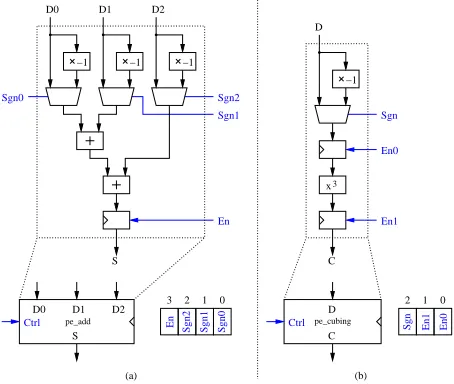
A. Addition and Subtraction overF3m
Since they are performed component-wise, addition and subtraction over F3m are rather straightforward operations. Each element ai of F3 is encoded by two bits aLi and a
H i
such that [18]: aLi = aimod 2 and aHi = ai div2. Thus,
the addition of ai and bi on a Cyclone-II FPGA requires
two 4-input LUTs. A nice property of this encoding is that the negation of ai is performed by swapping the bits aLi
and aH
i . Our processor includes an operator which adds or
subtracts up to three elements ofF3m and stores the result in a register (Figure 1a).
D1
Ctrl
Sgn0
Sgn1
Sgn2
3 2 1 0
En
C D
pe_cubing
Ctrl Sgn En1 En0
2 1 0 −1
x3 Sgn
En0
En1
D
C D0 D1 D2
S
Sgn0
En Sgn2
Sgn1
(b) (a)
−1 −1 −1
D2 D0
S
pe_add
B. Cubing over F3m andF36m
Cubing is also a pretty simple arithmetic operation. Since F36m is constructed as an extension field of F3m, the com-putation of R30 involved in Algorithm 2 is replaced by six cubing, six additions (or subtractions), and a negation over F3m. Indeed, by noting that:
σ3=−σ, (ρ2)3=ρ2−ρ+ 1,
ρ3=ρ+ 1, (σρ2)3=−σρ2+σρ−σ,and
(σρ)3=−σρ−σ,
we obtain
C3= (c0+c1σ+c2ρ+c3σρ+c4ρ2+c5σρ2)3
= (c30+c32+c34) + (−c31−c33−c35)σ+ (c32−c34)ρ
+ (−c33+c35)σρ+c34ρ2+ (−c35)σρ2,
whereC= (c0, c1, c2, c3, c4, c5)belongs toF36m. Let us now consider the computation ofb(x) =a(x)3over
F3m. We have:
b(x) =a(x)3=
m−1
X
i=0 aix3i
!
modf(x),
where f(x) is a degree m irreducible polynomial over F3. Since we set f(x) =x97+x12+ 2, a simple Maple or Pari program provides us with a closed formula for cubing over F3m:
b0=a93+a89+a0, b3=a94+a90+a1
b1=a65−a61, . . .
b2=a33, b96=a32.
The most complex operation involved in cubing is the addition of three elements of F3. Therefore, the critical path includes only two LUTs. Our pairing accelerator embeds a single cubing unit (Figure 1b) which computes either a(x)3 or (−a(x))3 according to a control bit. In order to guarantee a short critical path, the operator includes two pipeline stages. It is worth noticing that the only degree97irreducible trinomial over F3 allowing a simple cube root extraction [10] has a more complex closed formula for cubing. Thus, Algorithm 2 offers additional flexibility to select parameters leading to the smallest hardware operators.
C. Multiplication over F3m
We designed a Most Significant Element (MSE) first mul-tiplier over F3m based on a paper by Song and Parhi [19] to compute a(x)b(x) modf(x). At stepiwe compute a degree
(m+D−2) polynomialt(x)which is the sum of D partial products:
t(x) =
D−1
X
j=0
aDi+jxjb(x).
A degree(m+D−1)polynomials(x), updated according to the celebrated Horner’s rule, allows to accumulate the partial products:
s(x)←t(x) +xD·(s(x) modf(x)).
Thus, afterdm/Desteps, this algorithm returns a degree(m+ D−1) polynomial s(x), which is congruent with a(x)b(x)
modulof(x). The circuit described by Song and Parhi requires dedicated hardware to compute p(x) =s(x) modf(x) [19]. We suggest to achieve this final modulo f(x) reduction by performing an additional iteration witha−j = 0,1≤j≤D.
Sincet(x)is now equal to zero, we have:
s(x) =xD·(a(x)b(x) modf(x)).
Therefore, it suffices to consider the m most significant coefficients ofs(x)to get the result (Figure 2a):
p(x) =s(x)/xD.
Algorithm 3 summarizes this multiplication scheme. Synthesis results indicate that forD = 3andD = 4, such a multiplier requires respectively 1170 and 1560 LEs. According to our size constraint, up to ten multipliers can be included in our pairing accelerator.
Algorithm 3 MSE multiplication overF3m.
Require: A degree m monic polynomial f(x) = xm +
fm−1xm−1 +. . . +f1x+ f0, a degree n polynomial a(x), and a degree(m−1) polynomialb(x). We assume that a−j = 0, 1 ≤ j ≤ D. The algorithm requires
a degree (m +D −1) polynomial s(x) as well as a degree (m+D −2) polynomial t(x) for intermediate computations.
Ensure: p(x) =a(x)b(x) modf(x) 1: s(x)←0;
2: fori indm/De −1 downto −1 do
3: t(x)←
D−1
X
j=0
aDi+jxjb(x);
4: s(x)←t(x) +xD·(s(x) modf(x));
5: end for
6: p(x)←s(x)/xD;
Shu et al. proposed to reduce the partial products
xja
Di+jb(x) as well as xDp(x) modulo f(x) in order to
keep a degree (m−1) intermediate result [12] (Figure 2b). This approach avoids the extra clock cycle introduced by our algorithm at the price of a larger critical path. It also requires
D modulof(x)reductions instead of a single one. However, due to the irreducible polynomial over F3 and the values of D considered in this work, the hardware overhead is not significant.
s(x)
x2
PPG a2i a2i+1
x x2
mod f(x) Critical path
mod f(x) s(x) x PPG
a2i+1 a2i
x2
mod f(x)
0 1
b(x)
p(x) PPG a2i+1 a2i
x
mod f(x) x2
Critical path Critical
path
p(x) Register t(x)
b(x)
p(x)
(a) (b) (c)
b(x)
Final reduction
p(x) b(x)
PPG
PPG
PPG mod f(x)
Fig. 2. Three multipliers overF3m (D = 2). a) Improvement of the algorithm by Song and Parhi [19]. Algorithms proposed by b) Shuet al.[12], and c) Bertoni et al.[20]. A box labelledPPG denotes a Partial Product Generator. A box with rounded corners involves only wiring.
D. Multiplication over F36m
The cost of Algorithm 2 is dominated by the multiplication of R0 by R1 over F36m. By applying Karatsuba-Ofman’s algorithm (see for instance [22]) and taking advantage of the constant coefficients of R1, the product R0R1 could be computed in parallel by means of 13 multiplications and
50 additions (or subtractions) over F3m [23]. Two further multiplications are needed to compute ypyq as well as r02 (a straightforward modification of the scheduling of Algorithm 2 allows to computer2
0,ypyq, and R0R1 in parallel). However, according to our size constraints, it is impossible to imple-ment 15 multipliers on our target FPGA. Furthermore, our processor embeds only three adders over F3m and scheduling 50 additions could be a complex task. We propose here an algorithm which offers a better trade-off between the number of additions and multiplications.
Let A = a0+a1σ+a2ρ+a3σρ+a4ρ2+a5σρ2 and C=c0+c1σ+c2ρ+c3σρ+c4ρ2+c5σρ2be two elements of F36m. We write each coefficient ci as a sum of two elements
c(0)i and c(1)i ∈ F3m. Thanks to this notation we define the productC=A·(−r2
0+ypyqσ−r0ρ−ρ2)as follows:
c(0)0 =−a4r0−a2, c (1)
0 =−a0r20−a1ypyq,
c(0)1 =−a5r0−a3, c (1)
1 =a0ypyq−a1r02, c(0)2 =−a0r0−a4+c
(0) 0 , c
(1)
2 =−a2r20−a3ypyq,
c(0)3 =−a1r0−a5+c (0) 1 , c
(1)
3 =a2ypqq−a3r20, c(0)4 =−a2r0−a0−a4, c
(1)
4 =−a4r20−a5ypyq,
c(0)5 =−a3r0−a1−a5, c (1)
5 =a4ypyq−a5r02.
Note that computation of the c(0)i ’s, 0 ≤i ≤5, requires six multiplications over F3m and depends neither on r20 nor on ypyq. Thus, we can perform eight multiplications overF3m in parallel (r2
0, ypyq, and air0, 0 ≤i ≤ 5). Consider now c (1) 0 and c(1)1 and assume that (a0+a1), as well as (ypyq−r02), are stored in registers. Karatsuba-Ofman’s algorithm allows to
compute c(1)0 and c(1)1 by means of three multiplications and three additions overF3m:
c(1)0 =−a0r02−a1ypyq, (4)
c(1)1 =a0ypyq−a1r02
= (a0+a1)(ypyq−r02) +a0r20−a1ypyq. (5)
Therefore, the computation of the c(1)i ’s involves nine multi-plications over F3m, which can be carried out in parallel.
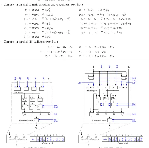
Algorithm 4 summarizes this multiplication scheme involv-ing17multiplications and 29additions (or subtractions) over F3m. Since at most nine multiplications can be performed in parallel, our pairing accelerator hosts nine multipliers over F3m and the computation ofR0R1involves two multiplication cycles. A careful scheduling allows to share operands between up to three operators, thus saving hardware resources (Table I):
• During the first multiplication cycle, M0, M1, and M2 respectively compute a0r0, a2r0, and a4r0. The MSE multiplier described in Section III-C stores its first operand in a shift register, and its second operand in a standard register. Since a shift register is more complex (an operand is loaded in parallel, and then shifted), we load the common operand r0 in this component. At the end of the first cycle, the three standard registers still containa0,a2, anda4. Therefore it suffices to loadr02in the shift register before starting the second multiplication cycle. Figure 3a describes the operator we designed. This component is connected to the addition/subtraction operator described in Section III-A (Figure 4).
• The same architecture allows to compute a1r0, a3r0, a5r0,a1ypyq,a3ypyq, anda5ypyq.
• The five remaining multiplications involve a slightly more complex component (Figure 3b). Two shift registers are required to compute r2
0 and ypyq since there is no
common operand. At the end of the first multiplication cycle, a dedicated subtracter computes ypyq −r02 and stores the result in the shift registers. Three clock cycles are requested to load(a0+a1),(a2+a3), and(a4+a5), which have been computed during the first multiplication cycle (see Algorithm 4).
This approach could also be adopted to implement the multi-plication ofR˜0by R˜1 in Algorithm 1.
TABLE I
MULTIPLICATION OVERF3m:SCHEDULING.
First cycle Second cycle
M0 a0·r0 a0·r20
M1 a2·r0 a2·r20
M2 a4·r0 a4·r20
M3 a1·r0 a1·ypyq
M4 a3·r0 a3·ypyq
M5 a5·r0 a5·ypyq
M6 r0·r0 (a0+a1)·(ypyq−r02)
M7 yp·yq (a2+a3)·(ypyq−r02)
Algorithm 4 Multiplication overF36m.
Require: A=a0+a1σ+a2ρ+a3σρ+a4ρ2+a5σρ2 ∈F36m.r0,yp, andyq ∈F3m.
Ensure: C=A·(−r2
0+ypyqσ−roρ−ρ2)
1: Compute in parallel (8 multiplications and 3 additions over F3m): pi ← air0, 0 ≤ i ≤ 5; p6 ← r0r0; p7 ← ypyq; s0←a0+a1; s1←a2+a3;s2←a4+a5;
2: Compute in parallel (7additions over F3m):
s4←p7−p6; //ypyq−r02 c3←a5+p1; //a5+a1r0
c0←a2+p4; // a2+a4r0 c4←a0+p2; //a0+a2r0
c1←a3+p5; // a3+a5r0 c5←a1+p3; //a1+a3r0
c2←a4+p0; // a4+a0r0
3: Compute in parallel (9multiplications and 4 additions overF3m):
p8←a0p6; // a0r02 p15←a5p7; // a5ypyq
p9←a1p7; // a1ypyq p16←s2s4; //(a4+a5)(ypyq−r02)
p10←s0s4; //(a0+a1)(ypyq−r02) c2←c2+c0; //a0r0+a4+a4r0+a2
p11←a2p6; // a2r02 c3←c3+c1; //a1r0+a5+a5r0+a3
p12←a3p7; // a3ypyq c4←c4+a4; // a2r0+a0+a4
p13←s1s4; //(a2+a3)(ypyq−r02) c5←c5+a5; // a3r0+a1+a5
p14←a4p6; // a4r02
4: Compute in parallel (15additions overF3m):
c0← −c0−p8−p9; c3← −c3+p13+p11−p12;
c1← −c1+p10+p8−p9; c4← −c4−p14−p15;
c2← −c2−p11−p12; c5← −c5+p16+p14−p15;
3 2 1 0 9 8 7 6 5 4
12 11 10
Sel1
Sel0 Rst1 Rst0 En1 En0 Shift Ld4 Ld3 Ld2 Ld1 Ld0
M0 M1 M2
Control word Sel
Rst1 Rst0 En1 En0 Shift Ld3 Ld2 Ld1 Ld0
Q
En1 Rst1 Sel En0 Rst0
00 01 10 11
Synchronous reset
Ld0 Ld1 Ld2
Ld3
Shift D0 D1
Shift register
00 01 10 11
En0 Rst0
En1 Rst1
Q
Sel1
Synchronous reset 0
1 1 0
Ld0 Ld1 Ld2
D0 D1
Sel0 Shift Ld4 Ld3
Shift register
Control word
(a) pe_mult_block_t1_generic (b) pe_mult_block_t2_generic M6 M7 M8
pe_mult_block_t1_generic
D1 D0
Q
Ctrl 10 9 8 7 6 5 4 3 2 1 0 D0 D1
Q Ctrl
pe_mult_block_t2_generic
E. Architecture of the Pairing Accelerator
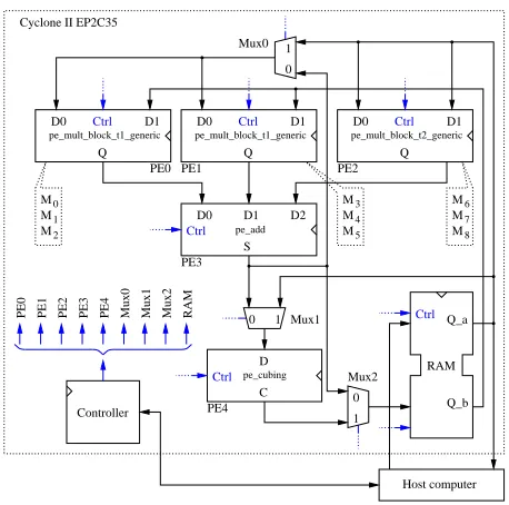
Figure 4 shows the architecture of our hardware accelerator. Inputs and outputs, as well as intermediate results, are stored in registers implemented using embedded memory blocks available in the FPGA.
The control unit mainly consists of a ROM containing the microcode of Algorithm 2 and a program counter. The size of the microcode depends on D, the number of coefficients processed at each clock cycle by a multiplier over F3m. For D = 3, the initialization step of Algorithm 2 (copy of inputs in registers of multipliers and computation of r0,d, andR0) and the main loop respectively require47and98clock cycles. Since m = 97, a pairing is completed after 47 + 98·(m−
1)/2 = 47 + 98·49 = 4849 clock cycles. For D = 4, the
initialization and the main loop respectively involve39and80
microinstructions. Thus, the computation of a pairing requires
39 + 80·49 = 3959clock cycles.
pe_add
D1
Ctrl
Mux1
0 1
0 1 Mux0
pe_mult_block_t1_generic
D1 D0
Q
Ctrl
Mux2
0 1
D1 D0
Q
Ctrl
pe_mult_block_t2_generic
RAM Q_a
Q_b M2
M1
M0
M8
M7
M6
Mux0 Mux1 Mux2 RAM PE0 PE1 PE2 PE3 PE4
Host computer Cyclone II EP2C35
C D
pe_cubing
Ctrl
Ctrl
Controller
M5
M4
M3
PE1
PE0 PE2
PE3
PE4
pe_mult_block_t1_generic
D1 D0
Q
Ctrl
D2 D0
S
Fig. 4. Architecture of theηT pairing accelerator.
IV. RESULTS ANDCOMPARISONS
The proposed architecture was captured in the VHDL lan-guage and prototyped on an Altera Cyclone II EP2C35F672C6 device. Both synthesis and place-and-route steps were per-formed with Quartus II 6.0 Web Edition. VHDL simulations and experiments with a DE2 board were carried out to exten-sively test our design. The area and the calculation time depend on D, the number of coefficients of a multiplier processed at each clock cycle (Section III-C). The two rightmost columns of Table II summarize our results for D = 3 and D = 4. When D = 3, the pairing accelerator occupies 45% of the LEs, thus meeting our size constraint (Section III). However, choosing D = 4 lead to an architecture which requires 56% of the configurable logic.
Several researchers described implementations of pairing al-gorithms on Xilinx Virtex-II Pro FPGAs and reported the area in terms ofslices. Each slice features two4-input LUTs, carry logic, wide function multiplexers, and two storage elements. Let us assume that Xilinx design tools try to utilize both LUTs of a slice as often as possible (i.e. area optimization). Under this hypothesis, we consider that a slice is roughly equivalent to two LEs in our comparisons.
To our best knowledge, the FPGA-based pairing accelerator described by Shu et al. in [12] is the fastest to date. It computes the Tate pairing over F2239 in 34 µs on a
Virtex-II Pro 100 device (25287 slices). Ronan et al. designed an embedded processor to compute the ηT pairing on genus
2 hyperelliptic curves [24]. This architecture requires 43986
slices on a Virtex-II Pro 125 device and computes a pairing in 749 µs. Kerins et al. proposed an implementation of the modified Duursma-Lee algorithm on a Xilinx Virtex-II Pro 125 FPGA [14]. Multiplication overF36m is performed according to Karatsuba-Ofman’s algorithm. However, since the authors do not take advantage of the constant terms of R1, this operation requires 18 multiplications over F3m. Thus, the hardware architecture consists of18 multipliers and6 cubing circuits over F397, along with “a suitable amount of simpler
F3m arithmetic circuits for performing addition, subtraction, and negation” [14]. The authors claim that roughly100% of available resources are required to implement their pairing accelerator. We can therefore estimate the cost to 55616
slices [12]. Remember that our target FPGA embeds 33216
LEs. Consequently, even if the final exponentiation unit we left for future work requires50% of the device, our processor is smaller than the aforementioned solutions. Furthermore, our approach requires a less expensive FPGA technology for which free simulation and design tools are available.
Grabher and Page designed a coprocessor dealing with F3m arithmetic, which is controlled by a general purpose processor [18]. Their hardware accelerator embeds a single multiplier over F3m. Our architecture requires roughly twice as much LEs, while performing up to nine multiplications in parallel.
Several researchers studied the software implementation of pairings on smartcards or mobile phones (see for instance [25] and [26]). For comparison purpose, they often provide the reader with timings on desktop computers. Table III summa-rizes such results which indicate that our FPGA architecture achieves a speedup of100.
TABLE III
COMPARISONS WITH SOFTWARE IMPLEMENTATIONS ON DESKTOP COMPUTERS.
Kawahara Scott Proposed
et al.[25] et al.[26] architecture
Algorithm ηT pairing ηT pairing Algorithm 2
Processor Pentium M Pentium 4 FPGA
Clock frequency 1.73GHz 3GHz 0.149GHz
TABLE II
COMPARISON AGAINST PREVIOUSFPGAIMPLEMENTATIONS. THE PARAMETERDREFERS TO THE NUMBER OF COEFFICIENTS PROCESSED AT EACH CLOCK CYCLE BY A MULTIPLIER.
Shu, Kwon, Ronanet al.[24] Grabher and Kerinset al.[14] Proposed architecture
and Gaj [12] Page [18] D=3 D=4
Algorithm ηT pairing ηTpairing Duursma-Lee Duursma-Lee Algorithm 2
Underlying field F2239 F2103 F397 F397 F397
Curve Elliptic Hyperelliptic Elliptic Elliptic Elliptic
FPGA Virtex-II Pro 100 Virtex-II Pro 125 Virtex-II Pro 4 Virtex-II Pro 125 Cyclone II EP2C35
Free design tools No No Yes No Yes
Controller Hardwired logic Hardwired logic Microprocessor Hardwired logic Hardwired logic
Multiplier(s) 6(overF2239) 12(overF2103) 1(overF397) 18(overF397) 9(overF397)
Area 25287slices 43986slices 4481slices 55616slices 14895LEs 18553LEs
Clock cycles – – – 12866 4849 3959
Clock frequency 84MHz 32.3MHz 150MHz 15MHz 149MHz 147MHz
Calculation time 34µs 749µs 399.4µs 850µs 33µs 27µs
Final exponentiation Yes Yes No Yes No No
V. CONCLUSIONS
We have proposed a modified ηT pairing algorithm on
supersingular elliptic curves over F3m which does not need any cube root. We have then described a pairing accelerator based on a low cost platform hosting an Altera Cyclone II FPGA. Since VHDL simulation and FPGA configuration are performed with free design tools, the price of our system is comparable to that of an entry level desktop computer. Our results demonstrate a one hundred-fold improvement on software implementations, and a ten-fold improvement on the best known FPGA implementation in characteristic three. We achieve the same calculation time than the fastest published accelerator in characteristic two, while requiring less hardware resources. Further work will include the design of a small processing unit responsible for final exponentiation.
ACKNOWLEDGEMENT
This work was supported by the New Energy and Industrial Technology Development Organization (NEDO), Japan.
REFERENCES
[1] D. Boneh and M. Franklin, “Identity-based encryption from the Weil pairing,” inAdvances in Cryptology – CRYPTO 2001, ser. Lecture Notes in Computer Science, J. Kilian, Ed., no. 2139. Springer, 2001, pp. 213– 229.
[2] D. Boneh, B. Lynn, and H. Shacham, “Short signatures from the Weil pairing,” inAdvances in Cryptology – ASIACRYPT 2001, ser. Lecture Notes in Computer Science, C. Boyd, Ed., no. 2248. Springer, 2001, pp. 514–532.
[3] D. Boneh, C. Gentry, and B. Waters, “Collusion resistant broadcast encryption with short ciphertexts and private keys,” in Advances in
Cryptology – CRYPTO 2005, ser. Lecture Notes in Computer Science,
V. Shoup, Ed., no. 3621. Springer, 2005, pp. 258–275.
[4] V. S. Miller, “Short programs for functions on curves,” 1986, unpublished manuscript available at http://crypto.stanford.edu/miller/miller.pdf.
[5] P. S. L. M. Barreto, H. Y. Kim, B. Lynn, and M. Scott, “Efficient algorithms for pairing-based cryptosystems,” inAdvances in Cryptology
– CRYPTO 2002, ser. Lecture Notes in Computer Science, M. Yung,
Ed., no. 2442. Springer, 2002, pp. 354–368.
[6] S. D. Galbraith, K. Harrison, and D. Soldera, “Implementing the Tate pairing,” inAlgorithmic Number Theory – ANTS V, ser. Lecture Notes in Computer Science, C. Fieker and D. Kohel, Eds., no. 2369. Springer, 2002, pp. 324–337.
[7] I. Duursma and H. S. Lee, “Tate pairing implementation for hyperelliptic curvesy2 =xp−x+d,” inAdvances in Cryptology – ASIACRYPT
2003, ser. Lecture Notes in Computer Science, C. S. Laih, Ed., no. 2894. Springer, 2003, pp. 111–123.
[8] S. Kwon, “Efficient Tate pairing computation for supersingular elliptic curves over binary fields,” 2004, cryptology ePrint Archive, Report 2004/303.
[9] K. Fong, D. Hankerson, J. L´opez, and A. Menezes, “Field inversion and point halving revisited,”IEEE Transactions on Computers, vol. 53, no. 8, pp. 1047–1059, Aug. 2004.
[10] P. S. L. M. Barreto, “A note on efficient computation of cube roots in characteristic 3,” 2004, cryptology ePrint Archive, Report 2004/305. [11] P. S. L. M. Barreto, S. Galbraith, C. ´O h ´Eigeartaigh, and M. Scott,
“Efficient pairing computation on supersingular Abelian varieties,” 2004, cryptology ePrint Archive, Report 2004/375.
[12] C. Shu, S. Kwon, and K. Gaj, “FPGA accelerated Tate pairing based cryptosystem over binary fields,” 2006, cryptology ePrint Archive, Report 2006/179.
[13] J. H. Silverman,The Arithmetic of Elliptic Curves, ser. Graduate Texts in Mathematics. Springer-Verlag, 1986, no. 106.
[14] T. Kerins, W. P. Marnane, E. M. Popovici, and P. Barreto, “Efficient hardware for the Tate Pairing calculation in characteristic three,” in
Cryptographic Hardware and Embedded Systems – CHES 2005, ser.
Lecture Notes in Computer Science, J. R. Rao and B. Sunar, Eds., no. 3659. Springer, 2005, pp. 412–426.
[15] K. Harrison, D. Page, and N. P. Smart, “Software implementation of finite fields of characteristic three, for use in pairing-based cryptosys-tems,”LMS Journal of Computation and Mathematics, vol. 5, pp. 181– 193, Nov. 2002.
[16] DE2 Development and Education Board – User Manual, Altera, 2006,
available from Altera’s web site (http://altera.com).
[17] Cyclone II Device Handbook, Altera, 2006, available from Altera’s web site (http://altera.com).
[18] P. Grabher and D. Page, “Hardware acceleration of the Tate Pairing in characteristic three,” inCryptographic Hardware and Embedded Systems
– CHES 2005, ser. Lecture Notes in Computer Science, J. R. Rao and
B. Sunar, Eds., no. 3659. Springer, 2005, pp. 398–411.
[19] L. Song and K. K. Parhi, “Low energy digit-serial/parallel finite field multipliers,”Journal of VLSI Signal Processing, vol. 19, no. 2, pp. 149– 166, July 1998.
[20] G. Bertoni, J. Guajardo, S. Kumar, G. Orlando, C. Paar, and T. Wollinger, “Efficient GF(pm)arithmetic architectures for cryptographic
applica-tions,” inTopics in Cryptology – CT-RSA 2003, ser. Lecture Notes in Computer Science, M. Joye, Ed., no. 2612. Springer, 2004, pp. 158– 175.
[21] S. Kumar, T. Wollinger, and C. Paar, “Optimum digit serial GF(2m)
multipliers for curve-based cryptography,”IEEE Transactions on Com-puters, vol. 55, no. 10, pp. 1306–1311, Oct. 2006.
[22] D. Zuras, “More on squaring and multiplying large integers,” IEEE
Transactions on Computers, vol. 43, no. 8, pp. 899–908, Aug. 1994.
the Third International Conference on Information Technology: New
Generations (ITNG’06). IEEE Computer Society, 2006.
[24] R. Ronan, C. ´O h ´Eigeartaigh, C. Murphy, M. Scott, T. Kerins, and W. Marnane, “An embedded processor for a pairing-based cryptosys-tem,” inProceedings of the Third International Conference on
Informa-tion Technology: New GeneraInforma-tions (ITNG’06). IEEE Computer Society,
2006.
[25] Y. Kawahara, T. Takagi, and E. Okamoto, “Efficient implementation of Tate pairing on a mobile phone using Java,” 2006, cryptology ePrint Archive, Report 2006/299.
[26] M. Scott, N. Costigan, and W. Abdulwahab, “Implementing crypto-graphic pairings on smartcards,” 2006, cryptology ePrint Archive, Report 2006/144.
APPENDIXI
RELATIONSHIP BETWEENηT(P, Q)W ANDˆe(P, Q)
According to Equation (2), we have:
ˆ
e(P, Q)−b3(m+3)/2=v3(−b3(m+1)/2−1)2,
where v denotes ηT(P, Q)W. Let us raise both sides of the
above equation to the−b3(m−3)/2-th power. Sinceb2= 1, we obtain:
ˆ
e(P, Q)3m =v3(−b3(m+1)/2−1)2(−b3(m−3)/2) =v3m(−2−b3(m+1)/2)−b3(m−1)/2.
Thus,
ˆ
e(P, Q) = 3 mp
v3m(−2−b3(m+1)/2)
·v−b3(m−1)/2 =v−2·v3(m+1)/2· 3mpv3(m−1)/2−b .
Algorithm 5 describes the implementation of the above equa-tion.
Algorithm 5 Computation of the modified Tate pairing.
Require: v = ηT(P, Q)W ∈ F36m. Three variables x0, x1, andx2 belonging toF36m store intermediate results.
Ensure: e(P, Q)ˆ
1: x0←v(3m−1)/2; //(m−1)/2 cubings 2: x1←v2; //1multiplication
3: x2←x30; //1cubing 4: x0← 3m
√
x0; //3m-th root 5: ifb= 1then
6: x0←x0·x1·x2; //2multiplications 7: x0←x−10 ; //1inversion
8: else
9: x0← x0x·x2
1 ; //1multiplication and1 division 10: end if
11: Returnx0;
APPENDIXII PROOF OFALGORITHM2
Assume that Algorithms 1 and 2 are provided with the same input (i.e. P = ˜P and Q= ˜Q). In order to prove the correctness of the scheme proposed in this paper, it suffices to show that:
R0[(m−1)/2] = ˜R0[(m−1)/2]3
(m+1)/2 ,
where[i]denotes the value of a variable at the end of theith iteration of Algorithms 1 and 2. The proof proceeds in three steps. After establishing some useful properties, we prove that:
R1[i] = ˜R1[i]3 i
. (6)
We conclude by showing that:
R0[i] = ˜R0[i]3 i+1
. (7)
A. Properties
The computation ofR˜1[i]3 i
requires that we raiseσ,ρ, and
ρ2 to the3i-th power. Since σ2=−1, we have:
σ3i =
(
σ ifi≡0 (mod 2),
−σ otherwise. (8)
From ρ3=ρ+b, we deduce that:
ρ3i=
ρ ifi≡0 (mod 3),
ρ+b ifi≡1 (mod 3),
ρ−b otherwise,
(9)
and
(ρ2)3i =
ρ2 ifi≡0 (mod 3),
ρ2−bρ+ 1 ifi≡1 (mod 3),
ρ2+bρ+ 1 otherwise.
(10)
We also need a relationship between r0[i] and r˜0[i]. Since P = ˜P, we easily check by induction that:
xp[i] = ˜xp[i]3
i+1
, yp[i] = (−1)i+1y˜p[i]3
i+1 ,
xq[i] = ˜xq[i]3
i+1
, and yq[i] = ˜yq[i]3
i+1 .
(11)
Remember now that r˜0[i] andr0[i] are respectively updated as follows:
˜
r0[i]←x˜p[i−1] + ˜xq[i−1] +b, and
r0[i]←xp[i−1] +xq[i−1] +d[i−1].
Therefore, according to Equation (11), we have:
r0[i] = ˜xp[i−1]3
i
+ ˜xq[i−1]3
i
+d[i−1].
We deduce the update rule ofd[i]from Algorithm 2:
d[i] =
0 ifi≡0 (mod 3),
−b ifi≡1 (mod 3),
b otherwise.
Thus,
r0[i] =
˜ r0[i]3
i
ifi≡0 (mod 3),
˜ r0[i]3
i
−b ifi≡1 (mod 3),
˜ r0[i]3
i
B. Relationship BetweenR1[i]and R˜1[i]
The most technical part of the proof consists in showing that Equation 6 holds. Recall thatR˜1[i]andR1[i]are updated as follows:
˜
R1[i]← −r˜0[i]2+ ˜yp[i−1]˜yq[i−1]σ−r˜0[i]ρ−ρ2, and
R1[j]← −r0[i]2+yp[i−1]yq[i−1]σ−r0[i]ρ−ρ2.
Therefore, we have to study six cases depending on i (see Table IV for details):
• i≡0 (mod 6):
˜ R1[i]3
i
= (−r˜0[i]2)3 i
+ ˜yp[i−1]3
i ˜
yq[i−1]3
i σ
−r˜0[i]3 i
ρ−ρ2
= −r0[i]2+yp[i−1]yq[i−1]σ
−r0[i]ρ−ρ2
= R1[i]
• i≡1 (mod 6):
˜ R1[i]3
i
= −(˜r0[i]2)3 i
−y˜p[i−1]3
i ˜
yq[i−1]3
i σ
−r˜0[i]3 i
(ρ+b)−ρ2+bρ−1
= (−(˜r0[i]3 i
)2−r˜0[i]3 i
b−1)
+yp[i−1]yq[i−1]σ−(˜r0[i]3 i
−b)ρ−ρ2
= (−(˜r0[i]3 i
)2+ 2˜r0[i]3 i
b−1)
+yp[i−1]yq[i−1]σ−r0[i]ρ−ρ2
Since b∈ {−1,1},b2= 1and we have:
(−(˜r0[i]3 i
)2−r˜0[i]3 i
b−1)
=−((˜r0[i]3 i
)2−2˜r0[i]3 i
b+b2)
=−(˜r0[i]3 i
−b)2=−r0[i]2.
Therefore,R˜1[i]3 i
=R1[i].
• i≡2 (mod 6):
˜ R1[i]3
i
= −(˜r0[i]2)3 i
+ ˜yp[i−1]3
i ˜
yq[i−1]3
i σ
−r˜0[i]3 i
(ρ−b)−ρ2−bρ−1
= (−(˜r0[i]3 i
)2+ ˜r0[i]3 i
b−1)
+yp[i−1]yq[i−1]σ−(˜r0[i]3 i
+b)ρ−ρ2
= −((˜r0[i]3 i
)2+ 2˜r0[i]3 j
b+b2)
+yp[i−1]yq[i−1]σ−r0[i]ρ−ρ2
= −(˜r0[i]3 j
+b)2
+yp[i−1]yq[i−1]σ−r0[i]ρ−ρ2
= R1[i]
• i≡3 (mod 6):
˜ R1[i]3
i
= (−r˜0[i]2)3 i
−y˜p[i−1]3
i ˜
yq[i−1]3
i σ
−r˜0[i]3 i
ρ−ρ2
= −r0[i]2+yp[i−1]yq[i−1]σ
−r0[i]ρ−ρ2
= R1[i]
• i≡4 (mod 6):
˜ R1[i]3
i
= −(˜r0[i]2)3 i
+ ˜yp[i−1]3
i ˜
yq[i−1]3
i σ
−r˜0[i]3 i
(ρ+b)−ρ2+bρ−1
= (−(˜r0[i]3 i
)2−˜r0[i]3 j
b−b2)
+yp[i−1]yq[i−1]σ−(˜r0[i]3 i
−b)ρ−ρ2
= −(˜r0[i]3 j
−b)2
+yp[i−1]yq[i−1]σ−r0[i]ρ−ρ2
= R1[i]
• j≡5 (mod 6):
˜ R1[i]3
i
= −(˜r0[i]2)3 i
−y˜p[i−1]3
i ˜
yq[i−1]3
i σ
−r˜0[i]3 i
(ρ−b)−ρ2−bρ−1
= (−(˜r0[i]3 i
)2+ ˜r0[i]3 i
b−1)
+yp[i−1]yq[i−1]σ−(˜r0[i]3 i
+b)ρ−ρ2
= −((˜r0[i]3 i
)2+ 2˜r0[i]3 i
b+b2)
+yp[i−1]yq[i−1]σ−r0[i]ρ−ρ2
= −(˜r0[i]3 i
+b)2
+yp[i−1]yq[i−1]σ−r0[i]ρ−ρ2
= R1[i]
Thus,R1[i] = ˜R1[i]3 i
.
C. Relationship BetweenR0[i] andR˜0[i]
We check easily that Equation (7) holds fori= 0. At stepi,
1≤i≤(m−1)/2, Algorithms 1 and 2 respectively compute:
˜
R0[i]←R˜0[i−1] ˜R1[i], and
R0[i]←(R0[i−1]R1[i])3.
Recall thatR1[i] = ˜R1[i]3 i
and assume thatR0[i] = ˜R0[i]3 i+1
. We show by induction that Equation (7) holds for anyi:
R0[i+ 1] = (R0[i]R1[i+ 1])3
= ( ˜R0[i]3 i+1
˜
R1[i+ 1]3 i+1
)3
= ( ˜R0[i] ˜R1[i+ 1])3 i+2
= ˜R0[i+ 1]3 i+2
.
We conclude the proof by substituting (m−1)/2 for i in Equation (7). We obtain:
R0[(m−1)/2] = ˜R0[(m−1)/2]3
(m+1)/2 .
APPENDIXIII
3m-THROOT OVERF36m
This Appendix describes an algorithm to compute B = 3m√
TABLE IV
COMPUTATION OFR1[i]FROMR˜1[i]3 i
.
i≡0 (mod 6) i≡1 (mod 6) i≡2 (mod 6) i≡3 (mod 6) i≡4 (mod 6) i≡5 (mod 6)
σ3i σ −σ σ −σ σ −σ
ρ3i ρ ρ+b ρ−b ρ ρ+b ρ−b
(ρ2)3i ρ2 ρ2−bρ+ 1 ρ2+bρ+ 1 ρ2 ρ2−bρ+ 1 ρ2+bρ+ 1
yp[i−1] yp˜ [i−1]3i −yp˜ [i−1]3i yp˜ [i−1]3i −yp˜ [i−1]3i yp˜ [i−1]3i −yp˜ [i−1]3i
r0[i] r˜0[i]3 i
˜
r0[i]3 i
−b ˜r0[i]3 i
+b r˜0[i]3
i
˜
r0[i]3 i
−b ˜r0[i]3 i
+b
According to Equations (8), (9), and (10), we haveσ3m
=−σ,
ρ3m
=ρ+ 1, and(ρ2)3n
=ρ2−ρ+ 1. Thus,
(b0,b1, b2, b3, b4, b5)3 m
= (b0+b1σ+b2ρ+b3σρ+b4ρ2+b5σρ2)3 m
=b0+b1σ3 m
+b2ρ3 m
+b3(σρ)3 m
+b4(ρ2)3 m
+b5(σρ2)3 m
= (b0+b2+b4) + (−b1−b3−b5)σ+ (b2−b4)ρ
+ (−b3+b5)σρ+b4ρ2+ (−b4)σρ2
= (a0, a1, a2, a3, a4, a5).
By solving this system of six equations, we obtain:
b0=a0−a2+a4,
b1=−a1+a3−a5, b2=a2+a4,
b3=−a3−a5, b4=a4,
b5=−a5.
APPENDIXIV
RAISINGηT(P, Q)TO THEW-TH POWER
Algorithm 6 describes a simple way to rise ηT(P, Q) (or
ηT(P, Q)3(m+1)/2) to theW-th power whenb= 1. To check
its correctness, it suffices to note that the intermediate variables
ui andvi are defined as follows:
u0=ηT(P, Q), u1=ηT(P, Q)2·3
m ,
u2=ηT(P, Q)3
2m
, u3=ηT(P, Q)3
3m ,
u4=ηT(P, Q)2·3
4m
, u5=ηT(P, Q)3
5m ,
v0=ηT(P, Q)3
(m+1)/2
, v1=ηT(P, Q)3
m+(m+1)/2 ,
v3=ηT(P, Q)3
3m+(m+1)/2
, v4=ηT(P, Q)3
4m+(m+1)/2 .
Thus,
u6=ηT(P, Q)3
(m+1)/2+3m+(m+1)/2+33m+2·34m+35m
and
v5=ηT(P, Q)1+2·3
m+32m+33m+(m+1)/2+34m+(m+1)/2 .
The algorithm returns u6/v5 which is equal to ηT(P, Q)W.
Since cubing and raising to the3m-th power require only a few additions over F3m, the cost of Algorithm 6 is dominated by ten multiplications and one division (or eleven multiplications and one inversion) overF36m.
Algorithm 6 RaisingηT(P, Q)to theW-th power (b= 1). Require: ηT(P, Q)∈F36m. Thirteen variablesui,0≤i≤6,
and vi, 0 ≤i ≤5 belonging to F36m store intermediate results.
Ensure: ηT(P, Q)W ∈F36m 1: u0←ηT(P, Q);
2: fori= 1to5 do
3: ui←u3
m
i−1; 4: end for
5: u1←u21; //1 multiplication 6: u4←u24; //1 multiplication 7: v0←ηT(P, Q)3
(m+1)/2
; //(m+ 1)/2 cubings
8: fori= 1to4 do
9: vi←v3
m
i−1; 10: end for
![Fig. 2.Three multipliers overalgorithm by Song and Parhi [19]. Algorithms proposed by b) Shuand c) Bertoni F3 m ( D=2 )](https://thumb-us.123doks.com/thumbv2/123dok_us/1850401.1240149/5.612.51.296.54.207/multipliers-overalgorithm-song-parhi-algorithms-proposed-shuand-bertoni.webp)