Distributed Algorithms in Large-scaled Empirical Risk Minimization: Non-convexity, Adaptive-sampling, and Matrix-free Second-order Methods

(1)

Lehigh University

Lehigh Preserve

Theses and Dissertations

2019

Distributed Algorithms in Large-scaled Empirical

Risk Minimization: Non-convexity,

Adaptive-sampling, and Matrix-free Second-order Methods

Xi He

Lehigh University, [email protected]

Follow this and additional works at:

https://preserve.lehigh.edu/etd

Part of the

Industrial Engineering Commons

This Dissertation is brought to you for free and open access by Lehigh Preserve. It has been accepted for inclusion in Theses and Dissertations by an authorized administrator of Lehigh Preserve. For more information, please [email protected].

Recommended Citation

He, Xi, "Distributed Algorithms in Large-scaled Empirical Risk Minimization: Non-convexity, Adaptive-sampling, and Matrix-free Second-order Methods" (2019).Theses and Dissertations. 4352.

(2)

Distributed Algorithms in Large-scaled Empirical Risk

Minimization: Non-convexity, Adaptive Sampling, and

Matrix-free Second-order Methods

by

Xi He

Presented to the Graduate and Research Committee of Lehigh University

in Candidacy for the Degree of Doctor of Philosophy

in

Industrial and Systems Engineering

Lehigh University January 2019

(3)

c

(4)

Approved and recommended for acceptance as a dissertation in partial fulfillment of the requirements for the degree of Doctor of Philosophy.

Date

Dr. Martin Takáč, Dissertation Advisor

Committee Members:

Dr. Martin Takáč, Committee Chair

Dr. Katya Scheinberg

Dr. Frank E. Curtis

(5)

Acknowledgments

Firstly, I would like to express my sincere gratitude to my advisor Dr. Martin Takáč for his continuous support of my overall Ph.D. process, for his patience, motivation, immense knowledge and brainstorm ideas. I would never forget the very first time when he helped me accelerate my naive code to let it run ten times faster, like a magic. Dr. Martin Takáč is not only an advisor for me, but a mentor for many aspects in my life. All the relevant research and this dissertation are certainly impossible to complete without the constant and generous help from him.

Besides my advisor, I would also thank all my dissertation committee members: Dr. Katya Scheinberg, Dr. Frank E. Curtis, and Dr. Martin Jaggi, not only for your insightful com-ments and encouragement, but the hard questions which help me to understand and widen my research in various perspectives. My deep thanks would also go to our Optimization and Machine Learning (OptML) group at Lehigh University. I always feel extremely lucky to be a member of OptML, where I’m able to exchange ideas and discuss interests with all members. Without the year by year’s weekly seminar and insightful discussion, I would be definitely not able to build my addictive interests in the field of optimization.

I’m also grateful to Rachael Tappenden, Albert Berahas, and Dheevatsa Mudiger. With all their endless help, I would be able to stay on the right track towards my interests. Also, I would like to especially thank Ioannis Akrotirianakis, Amit Chakraborty, Neo Hsin-Chan Huang, Shuo Li, Eric Zhu, Maxence G Hardy, who provided me opportunities to join their team as an intern. With more touch of real-world applications matching what I have learned, I would, therefore, be clear on my future direction.

(6)

Yinan Liu, Rui Shi, Miao Bai, Choat Inthawongse, Mohammadreza Samadi, Hiva Ghanbari, and many others. I can’t stop to recall all the fun we have had in the last several years and all their support and kindness, they make my life at Bethlehem so wonderful. I would also borrow the place to thank my previous advisor, Qingzhi Yang and all my friends back at Nankai University, China. Without your encouragement and understanding, any of the overseas life would not happen.

Finally, I am deeply indebted to my family for their tremendous love and consistently sup-porting of all my decisions. They have been always with me throughout my whole Ph.D. period. Wishing you all my family and friends good health and happiness forever.

(7)

List of Tables

1.1 A list of datasets used in the numerical experiments, see [11]. . . 23

3.1 A list of datasets used in the numerical experiments. . . 65

C.1 A list of datasets used in the numerical experiments. . . 128

(12)

List of Figures

1.1 Toy demo illustrating how to obtain a non-uniform mini-batch sampling with batch sizeb= 2 fromn= 4 coordinates. . . 20 1.2 A comparison of the number of epochs versus the duality gap for the various

algorithms. . . 25 1.3 A comparison of the number of epochs versus the relative primal object value

for SGD, dfSDCA, adfSDCA(+) and SVRG. . . 26 1.4 Comparing absolute value of dual residuals at each epoch between dfSDCA

and adfSDCA. . . 27 1.5 Comparing the number of iterations of various batch size on different losses. . 28 1.6 Comparing adfSDCA for two cases on quadratic loss. . . 29

2.1 Model (left) and data (right) parallelism. . . 33 2.2 A simple 2D example which has one saddle point (0,0) and two local

mini-mizer(0,1)and (0,−1). . . 37 2.3 Performance comparison among SGD and Hessian-free variants. . . 39 2.4 Performance comparison among various size of mini-batches on different

meth-ods (3 plots above). The neural network has two hidden layers with size 400, 150. . . 40 2.5 Number of iterations required to obtain training error 0.02 as a function of

batch size for second order methods. . . 41 2.6 Performance scaling of different part in distributed HF on upto 32 nodes

(13)

3.1 Evolution of angles between two adjacent iterative points (bottom row) and the corresponding optimization performance of SINTR and SINTR+. . . 64 3.2 Objective value and Training error evolution on various methods on

sub-cifra10 dataset starting with a nearly saddle point. . . 65 3.3 Objective value, Gradient norm and Training error evolution on SINTR+ and

ASGD in first 300 iterations . . . 66 3.4 Second order methods will converge to flatter minimizer. The first row is the

result for CIFRA10 and the second is result of MNIST. . . 67 3.5 The evolution of eigenvalues for SINTR+ and ASGD on sub-mnist dataset . . 68 3.6 Objective value and Training error evolution on various methods. . . 69 3.7 The distribution of eigenvalues for SINTR+ on sub-MNIST dataset. . . 70 3.8 The distribution of eigenvalues for SINTR+ on sub-CIFRA10 dataset. . . 70

4.1 Performance of different algorithms on a Logistic Regression problem with rcv1 as dataset. . . 83 4.2 Comparison between DANCE and SGD with various hyper-parameters

set-ting on Cifar10 dataset and vgg11 network. . . 85 4.3 Comparison between DANCE and Adam on Mnist dataset and NaiveCNet. . 86 4.4 Performance of DANCE algorithm with different number of computing nodes. 88

C.1 Performance of different algorithms on a Logistic Regression problem with gisette as dataset. . . 129 C.2 Comparison between DANCE and SGD with various hyper-parameters on

Mnist dataset and NaiveCNet. . . 130 C.3 Comparison between DANCE and with momentum for various hyper-parameters

on Cifar10 dataset and vgg11 network. . . 131 C.4 Comparison between DANCE and SGD with momentum for various

(14)

Abstract

The rising amount of data has changed the classical approaches in statistical modeling significantly. Special methods are designed for inferring meaningful relationships and hid-den patterns from these large datasets, which build the foundation of a study called Ma-chine Learning (ML). Such ML techniques have already applied widely in various areas and achieved compelling success.

In the meantime, the huge amount of data also requires a deep revolution of current tech-niques, like the availability of advanced data storage, new efficient large-scale algorithms and their distributed/parallelized implementation.

There is a broad class of ML methods can be interpreted as Empirical Risk Minimization (ERM) problems. When utilize various loss functions and likely necessary regularization terms, one could approach their specific ML goals by solving ERMs as separable finite sum optimization problems. There are circumstances where nonconvex component is introduced into the ERMs which usually makes the problems hard to optimize. Especially, in recent years, neural networks, a popular branch of ML, draw numerous attention from community. Neural networks are powerful and highly flexible inspired by the structured functionality of the brain. Typically, neural networks could be treated as large-scale and highly nonconvex ERMs.

While as nonconvex ERMs become more complex and larger in scales, optimization using stochastic gradient descent (SGD) type methods proceeds slowly regarding its convergence rate and incapability of being distributed efficiently. It motivates researchers to explore more advanced local optimization methods such as approximate-Newton/second-order methods. In this dissertation, first-order stochastic optimization for the regularized ERMs in Chapter1

(15)

is studied. Based on the development of stochastic dual coordinate accent (SDCA) method, a dual free SDCA with non-uniform mini-batch sampling strategy is investigated [30, 29]. We also introduce several efficient algorithms for training ERMs, including neural networks, using second-order optimization methods in a distributed environment. In Chapter 2, we propose a practical distributed implementation for Newton-CG methods. It makes training neural networks by second-order methods doable in the distributed environment [28]. In Chapter 3, we further build steps towards using second-order methods to train feed-forward neural networks with negative curvature direction utilization and momentum acceleration. In this Chapter, we also report numerical experiments for comparing second-order methods and first-order methods regarding training neural networks . The following Chapter 4 pur-pose an distributed accumulative sample-size second-order methods for solving large scale convex ERMs and nonconvex neural networks [35]. In Chapter 5, a python library named UCLibrary is briefly introduced for solving unconstrained optimization problems. This dis-sertation is all concluded in the last Chapter 6.

(16)

Chapter 1

Dual Free Adaptive Mini-batch

SDCA for Empirical Risk

Minimization

1.1

Introduction

In this chapter we study the `2-regularized Empirical Risk Minimization (ERM) problem,

which is widely used in the field of machine learning. The problem can be stated as follows. Given training examples (x1, y1), . . . ,(xn, yn) ∈ Rd×R, loss functions φ1, . . . , φn :R→ R

and a regularization parameter λ > 0, `2-regularized ERM is an optimization problem of

the form min w∈_RdP(w) := 1 n n X i=1 φi(wTxi) + λ 2kwk 2_, _(1.1)

where the first term in the objective function is a data fitting term and the second is a

regularization term that prevents over-fitting.

Many algorithms have been proposed to solve problem (1.1) over the past few years, including SGD, [84], SVRG and S2GD, [36, 64, 40] and SAG/SAGA, [79, 18, 76]. However, another very popular approach to solving `2-regularized ERM problems is to consider the

(17)

max α∈_RnD(α) :=− 1 n n X i=1 φ∗_i(−αi)− λ 2k 1 λnX T_α_k2_, _(1.2)

whereXT = [x1, . . . , xn]∈Rd×nis the data matrix andφ∗i denotes the Fenchel conjugate

of φi, namely, φ∗i(u) = maxz(zu−φi(z)). It is also known that P(w∗) = D(α∗), which

implies that for all w and α, we have P(w) ≥ D(α), and hence the duality gap, defined to be P(w(α))−D(α), can be regarded as an upper bound on the primal sub-optimality

P(w(α))−P(w∗). The structure of the dual formulation (1.2) makes it well suited to a multi-core or distributed computational setting, and several algorithms have been developed to take advantage of this including [32] [93, 34, 49, 94, 73, 13, 104].

A popular method for solving (1.2) is Stochastic Dual Coordinate Ascent (SDCA). The algorithm proceeds as follows. At iterationt of SDCA a coordinatei∈ {1, . . . , n}is chosen uniformly at random and the current iterateα(t) is updated toα(t+1) :=α(t)+δ∗ei, where

δ∗ = arg maxδ∈RD(α(t) +δei). Much research has focused on analysing the theoretical

complexity of SDCA under various assumptions imposed on the functions φ∗_i, including the pioneering work of Nesterov in [60] and others including [75, 95, 58, 57, 47, 94, 93].

A modification that has led to improvements in the practical performance of SDCA is the use of importance sampling when selecting the coordinate to update. That is, rather than using uniform probabilities, instead coordinate i is sampled with an arbitrary probability

pi, see for example [105, 13].

In many cases algorithms that employ non-uniform coordinate sampling outperform naïve uniform selection, and in some cases help to decrease the number of iterations needed to achieve a desired accuracy by several orders of magnitude, see for example [105, 13].

Notation and Assumptions. In this chapter we use the notation [n] def= {1, . . . , n},

as well as the following assumption. For alli∈ [n], the loss functionφi is L˜i-smooth with

˜

Li >0, i.e., for any given β, δ∈R, we have

|φ0_i(β)−φ0_i(β+δ)| ≤L˜i|δ|. (1.3)

(18)

∀w,w¯∈_Rd _{and for all}_i_∈_[_n_]_{there exists a constant} _L

i ≤ kxik2L˜i such that

k∇φi(xTi w)− ∇φi(xiTw¯)k ≤Likw−w¯k. (1.4)

We will use the notation

L= max 1≤i≤nLi, and ˜ L= max 1≤i≤n ˜ Li. (1.5)

Throughout this chapter we let _R₊ denote the set of nonnegative real numbers and we let

Rn+denote the set ofn-dimensional vectors with all components being real and nonnegative.

1.1.1 Contributions

In this section the main contributions of this chapter are summarized (not in order of significance).

Adaptive SDCA. We modify the dual free SDCA algorithm proposed in [83] to allow

for the adaptive adjustment of probabilities and a non-uniform selection of coordinates. Note that the method is dual free, and hence in contrast to classical SDCA, where the update is defined by maximizing the dual objective (1.2), here we define the update slightly differently (see Section 1.2 for details).

Allowing non-uniform selection of coordinates from an adaptive probability distribution leads to improvements in practical performance and the algorithm achieves a better conver-gence rate than in [83]. In short, we show that the error after T iterations is decreased by a factor ofQT

t=1(1−θ(t))≥(1−θ

∗₎T _{on average, where}_θ∗ _{is an uniformly lower bound for}

all θ(t). Here 1−θ(t) ∈(0,1) is a parameter that depends on the current iterate α(t) and the nonuniform probability distribution. By changing the coordinate selection strategy from uniform selection to adaptive, each1−θ(t)becomes smaller, which leads to an improvement in the convergence rate.

Non-uniform sampling procedure. Rather than using a uniform sampling of

co-ordinates, which is the commonly used approach, here we propose the use of non-uniform sampling from an adaptive probability distribution. With this novel sampling strategy, we

(19)

are able to generate non-uniform non-overlapping and proper (see Section 1.5) samplings for arbitrary marginal distributions under only one mild assumptions. Indeed, we show that without the assumption, there is no such non-uniform sampling strategy. We also extend our sampling strategy to allow the selection of mini-batches.

Better convergence and complexity results. By utilizing an adaptive probabilities

strategy, we can derive complexity results for our new algorithm that, for the case when every loss function is convex, depend only on theaverage of the Lipschitz constantsLi. This

improves upon the complexity theory developed in [83] (which uses a uniform sampling) and [14] (which uses an arbitrary but fixed probability distribution), because the results in those works depend on the maximum Lipschitz constant. Furthermore, even though adaptive probabilities are used here, we are still able to retain the very nice feature of the work in [83], and show that the variance of the update naturally goes to zero as the iterates converge to the optimum without any additional computational effort or storage costs. Our adaptive probabilities SDCA method also comes with an improved bound on the variance of the update in terms of the sub-optimality of the current iterate.

Practical aggressive variant. Following from the work of [13], we propose an efficient

heuristic variant of adfSDCA. For adfSDCA the adaptive probabilities must be computed at every iteration (i.e., once a single coordinate has been selected), which can be computa-tionally expensive. However, for our heuristic adfSDCA variant the (exact/true) adaptive probabilities are only computed once at the beginning of each epoch (where an epoch is one pass over the data/n coordinate updates), and during that epoch, once a coordinate has been selected we simply reduce the probability associated with that coordinate so it is not selected again during that epoch. Intuitively this is reasonable because, after a coordinate has been updated the dual residue associated with that coordinate decreases and thus the probability of choosing this coordinate should also reduce. We show that in practice this heuristic adfSDCA variant converges and the computational effort required by this algorithm is lower than adfSDCA (see Sections 1.4 and 1.6).

Mini-batch variant. We extend the (serial) adfSDCA algorithm to incorporate a

mini-batch scheme. The motivation for this approach is that there is a computational cost associated with generating the adaptive probabilities, so it is important to utilize them

(20)

effectively. We develop a non-uniform mini-batch strategy that allows us to update multiple coordinates in one iteration, and the coordinates that are selected have high potential to decrease the sub-optimality of the current iterate. Further, we make use of ESO framework (Expected Separable Overapproximation) (see for example [74], [73]) and present theoretical complexity results for mini-batch adfSDCA. In particular, for mini-batch adfSDCA used with batchsizeb, we derive the optimal probabilities to use at each iteration, as well as the best step-size to use to guarantee speedup.

1.1.2 Outline

This chapter is organized as follows. In Section 1.2 we introduce our new Adaptive Dual Free SDCA algorithm (adfSDCA), and highlight its connection with a reduced variance SGD method. In Section 1.3 we provide theoretical convergence guarantees for adfSDCA in the case when all loss functions φi(·) are convex, and also in the case when individual loss

functions are allowed to be nonconvex but the average loss functions Pn

i=1φi(·) is convex.

Section 1.4 introduces a practical heuristic version of adfSDCA, and in Section 1.5 we present a mini-batch adfSDCA algorithm and provide convergence guarantees for that method. Finally, we present the results of our numerical experiments in Section 1.6. Note that the proofs for all the theoretical results developed in this chapter are left to the appendix.

1.2

The Adaptive Dual Free SDCA Algorithm

In this section we describe the Adaptive Dual Free SDCA (adfSDCA) algorithm, which is motivated by the dual free SDCA algorithm proposed by [83]. Note that in dual free SDCA two sequences of primal and dual iterates, {w(t)}∞_t₌₀ and {α(t)}∞_t₌₀ respectively, are maintained. At every iteration of that algorithm, the variable updates are computed in such a way that the well known primal-dual relational mapping holds; for every iterationt:

w(t)= 1 λn Xn i=1α (t) i xi. (1.6)

(21)

Definition 1.2.1 (Dual residue, [13]). The dual residue κ(t)= (κ₁(t), . . . , κ(nt))T ∈Rn

asso-ciated with (w(t), α(t)) is given by:

κ(_it)def= α(_it)+φ0_i(xT_i w(t)). (1.7) The Adaptive Dual Free SDCA algorithm is outlined in Algorithm 1.1 and is described briefly now; a more detailed description (including a discussion of coordinate selection and how to generate appropriate selection rules) will follow. An initial solution α(0) is chosen, and then w(0) is defined via (1.6). In each iteration of Algorithm 1.1 the dual residue κ(t)

is computed via (1.7), and this is used to generate a probability distribution p(t). Next, a coordinatei∈[n]is selected (sampled) according to the generated probability distribution and a step of sizeθ(t)_∈₍₀_,₁₎_{is taken by updating the} _i_{th coordinate of} _α _via

α(_it+1) =α(_it)−θ(t)(p(_it))−1κ(_it). (1.8) Finally, the vectorw is also updated

w(t+1)=w(t)−θ(t)(nλp_i(t))−1κ(_it)xi, (1.9)

and the process is repeated. Note that the updates toα andwusing the formulas (1.8) and (1.9) ensure that the equality (1.6) is preserved.

Also note that the updates in (1.8) and (1.9) involve a step size parameter θ(t), which will play an important role in our complexity results. The step size θ(t) should be large so that good progress can be made, but it must also be small enough to ensure that the algorithm is guaranteed to converge. Indeed, in Section 1.3.1 we will see that the choice of

θ(t) depends on the choice of probabilities used at iterationt, which in turn depend upon a particular function that is related to the suboptimality at iterationt.

The dual residue κ(t) is informative and provides a useful way of monitoring subop-timality of the current solution (w(t), α(t)). In particular, note that if κi = 0 for some

coordinatei, then by (1.7) αi =−φ0i(wTxi), and substituting κi into (1.8) and (1.9) shows

(22)

Algorithm 1.1 Adaptive Dual Free SDCA (adfSDCA) 1: Input: Data: {xi, φi}ni=1 2: Initialization: Choose α(0) ∈_Rn 3: Setw(0)= _λn1 Pn i=1α (0) i xi 4: fort= 0,1,2, . . . do

5: Calculate dual residualκ(_it)=φ0_i(xT_i w(t)) +α(_it), for alli∈[n]

6: Generate adaptive probability distribution p(t) ∼κ(t)

7: Sample coordinateiaccording top(t)

8: Set step-sizeθ(t)∈(0,1)as in (1.20) 9: Update: α_i(t+1) =α(_it)−θ(t)(p(_it))−1κ(_it) 10: Update: w(t+1)₌_w(t)₋_θ(t)₍_nλp(t) i )−1κ (t) i xi 11: end for

On the other hand, a large value of |κi| (at some iteration t) indicates that a large step

will be taken, which is anticipated to lead to good progress in terms of improvement in sub-optimality of current solution.

The probability distributions used in Algorithm 1.1 adhere to the following definition.

Definition 1.2.2. (Coherence, [13]) Probability vector p∈_Rn _{is coherent with dual residue}

κ ∈ _Rn _{if for any index} _i _{in the support set of} _{κ, denoted by} _I

κ := {i∈ [n] : κi 6= 0}, we

havepi>0. Wheni /∈Iκ then pi = 0. We usep∼κ to represent this coherent relation.

1.2.1 Adaptive dual free SDCA as a reduced variance SGD method.

Reduced variance SGD methods have became very popular in the past few years, see for example [41, 36, 76, 18]. It is show in [83] that uniform dual free SDCA is an instance of a reduced variance SGD algorithm (the variance of the stochastic gradient can be bounded by some measure of sub-optimality of the current iterate) and a similar result applies to adfSDCA in Algorithm 1.1. In particular, note that conditioned onα(t−1), we have

E[w(t)|α(t−1)] (1.9) = w(t−1)−θ (t−1) λ n X i=1 pi npi ∇φi(xTi w(t −1)_{) +}_α(t−1) i xi (1.6) = w(t−1)−θ (t−1) λ ∇1 n n X i=1 φi(xTi w(t−1)) +λw(t−1) (1.1) = w(t−1)−θ (t−1) λ ∇P(w (t−1)₎_. _(1.10)

(23)

Combining (1.9) and (1.10) and replacet−1 byt gives E 1 npi κ(_it)xi|α(t) =∇P(w(t)), (1.11) which implies that _np1

iκ

(t)

i xi is an unbiased estimator of∇P(w(t)). Therefore, Algorithm 1.1

is eventually a variant of the Stochastic Gradient Descent method. However, we can prove (see Corollary 1.3.4 and Corollary 1.3.7) that the variance of the update goes to zero as the iterates converge to an optimum, which is not true for vanilla Stochastic Gradient Descent.

1.3

Convergence Analysis

In this section we state the main convergence results for adfSDCA (Algorithm 1.1). The analysis is broken into two cases. In the first case it is assumed that each of the loss functions

φi is convex. In the second case this assumption is relaxed slightly and it is only assumed

that the average of theφi’s is convex, i.e., individual functionsφi(·)for some (several)i∈[n]

are allowed to be nonconvex, as long as 1_nPn

j=1φj(·)is convex. The proofs for all the results

in this section can be found in the Appendix.

1.3.1 Case I: All loss functions are convex

Here we assume that φi is convex for alli∈[n]. Define the following parameter

γ def= λL,˜ (1.12)

whereL˜is given in (1.5). It will also be convenient to define the following potential function. For all iterationst≥0,

D(t)def= _n1kα(t)−α∗k2+γkw(t)−w∗k2. (1.13) The potential function (1.13) plays a central role in the convergence theory presented in this chapter. It measures the distance from the optimum in both the primal and (pseudo) dual variables. Thus, our algorithm will generate iterates that reduce this suboptimality

(24)

and therefore push the potential function toward zero. Also define

videf= kxik2 for alli∈[n]. (1.14)

We have the following result.

Lemma 1.3.1. Let L,˜ κ(_it), γ, D(t), andvi be as defined in (1.5), (1.7), (1.12), (1.13)and

(1.14), respectively. Suppose thatφi isL-smooth and convex for all˜ i∈[n]and let θ∈(0,1).

Then at every iteration t ≥0 of Algorithm 1.1, a probability distribution p(t) that satisfies

Definition 1.2.2 is generated and

ED(t+1)|α(t)−(1−θ)D(t)≤ n X i=1 −θ n 1− θ p(_it) + θ 2_v iγ n2_λ2_p(t) i ! (κ(_it))2. (1.15) Note that if the right hand side of (1.15) is negative, then the potential function decreases (in expectation) in iterationt:

ED(t+1)|α(t)≤(1−θ)D(t). (1.16)

The purpose of Algorithm 1.1 is to generate iterates (w(t)_{, α}(t)₎ _{such that the above holds.}

To guarantee negativity of the right hand term in (1.15), or equivalently, to ensure that (1.16) holds, consider the parameter θ. Specifically, any θ that is less than the function

Θ(·,·) :Rn+×Rn+→Rdefined as Θ(κ, p)def= nλ 2P i∈Iκκ 2 i P i∈Iκ(nλ 2₊_v iγ)p−i 1κ2i , (1.17)

will ensure negativity of the right hand term in (1.15). Moreover, the larger the value ofθ, the better progress Algorithm 1.1 will make in terms of the reduction inD(t). The functionΘ

depends on the dual residueκ and the probability distributionp. Maximizing this function w.r.t. p will ensure that the largest possible value ofθ can be used in Algorithm 1.1. Thus, we consider the following optimization problem:

max p∈_Rn +, P i∈Iκpi=1 Θ(κ, p). (1.18)

(25)

One may naturally be wary of the additional computational cost incurred by solving the optimization problem in (1.18) at every iteration. Fortunately, it turns out that there is an (inexpensive) closed form solution, as shown by the following Lemma.

Lemma 1.3.2. Let Θ(κ, p) be defined in (1.17). The optimal solution p∗(κ) of (1.18) is

p∗_i(κ) = p viγ+nλ2|κi| P j∈Iκ p vjγ+nλ2|κj| , for all i= 1, . . . , n. (1.19)

The corresponding θ by using the optimal solution p∗ is

θ= Θ(κ, p∗) = nλ 2P i∈Iκκ 2 i (P i∈Iκ p viγ+nλ2|κi|)2 . (1.20)

Proof. This can be verified by deriving the KKT conditions of the optimization problem in

(1.18). The details are moved to Appendix for brevity.

The results in [14] are weaker because they require a fixed sampling distribution p

throughout all iterations. Here we allow adaptive sampling probabilities as in (1.19), which enables the algorithm to utilize the data information more effectively, and hence we have a better convergence rate. Furthermore, the optimal probabilities found in [13] can be only applied to a quadratic loss function, whereas our results are more general because the optimal probabilities in (1.19) can used whenever the loss functions are convex, or when individual loss functions are non-convex but the average of the loss functions is convex (see Section 1.3.2).

Before proceeding with the convergence theory we define several constants. Let

C0

def

= _n1kα(0)−α∗k2₊_γ_k_w(0)₋_w∗_k2_, _(1.21)

whereγ is defined in (1.12). Note thatC0in (1.21) is equivalent to the value of the potential

function (1.13) at iteration t= 0, i.e.,C0 ≡D(0). Moreover, let

M def= Q1 + γQ λ2_n where Qdef= 1 n n X i=1 kxik2 (1.14) = 1 n n X i=1 vi. (1.22)

(26)

Theorem 1.3.3. Let L,˜ κ(_it), γ, D(t), vi, C0 and Q be as defined in (1.5), (1.7), (1.12),

(1.13), (1.14), (1.21) and (1.22), respectively. Suppose that φi is L-smooth and convex for˜

all i∈[n], letθ(t)∈(0,1) be decided by (1.20)for all t≥0 and let p∗ be defined via (1.19).

Then, setting p(t) =p∗ at every iteration t≥0 of Algorithm 1.1, gives

E[D(t+1)|α(t)]≤(1−θ∗)D(t), (1.23) where θ∗ def= nλ 2 Pn i=1(viγ+nλ2) ≤θ(t). (1.24) Moreover, for >0, if T ≥ n+LQ˜ λ log (λ+L)C0 2λL˜ , (1.25) then _E[P(w(T))−P(w∗)]≤.

Similar to [83], we have the following corollary which bounds the quantity_E[k 1

npiκ

(t)

i xik2]

in terms of the sub-optimality of the points α(t) and w(t) by using optimal probabilities.

Corollary 1.3.4. Let the conditions of Theorem 1.3.3 hold. Then at every iteration t≥0

of Algorithm 1.1, E   κ(_it)xi npi 2 |α(t−1)  ≤2M(E[kα(t)−α ∗_k2_|_α(t−1)_{] +}_L E[kw(t)−w∗k2|α(t−1)]).

Note that Theorem 1.3.3 can be used to show that both E[kα(t)−α∗k2]and E[kw(t)−

w∗k2_] _{go to zero as} _e−θ∗t_{. We can then show that}

E[k_np1_iκ_i(t)xik2] ≤ as long as t ≥

˜

O(_θ1∗log(1)). Furthermore, we achieve the same variance reduction rate as shown in [83],

i.e., _E[k 1

npiκ

(t)

i xik2]∼O˜(kκ(t)k2).

For the dual free SDCA algorithm in [83] where uniform sampling is adopted, the param-eter θ should be set to at mostmin λ

λn+ ˜L, where L˜ ≥maxivi·L. However, from Corollary

1.3.3, we know that thisθ is smaller than θ∗, so dual free SDCA will have a slower conver-gence rate than our algorithm. In [14], where they use a fixed probability distribution pi

for sampling of coordinates, they must chooseθ less than or equal to mini _L_ip_vi_inλ₊_nλ. This is

(27)

1.1, at any iteration t, we have thatθ(t) is greater than or equal to θ∗, which again implies that our convergence results are better.

1.3.2 Case II: The average of the loss functions is convex

Here we follow the analysis in [83] and consider the case where individual loss functionsφi(·)

for i∈[n]are allowed to be nonconvex as long as the average _n1Pn

j=1φj(·) is convex. First

we define several parameters that are analogous to the ones used in Section 1.3.1. Let

¯ γ def= 1 n n X i=1 L2_i, (1.26)

where Li is given in (1.4), and define the following potential function. For all iterations

t≥0, let

¯

D(t)def= 1 nkα

(t)₋_α∗_k2_{+ ¯}_γ_k_w(t)₋_w∗_k2_. _(1.27)

We also define the following constants

¯ C0def= 1 nkα (0)₋_α∗_k2_{+ ¯}_γ_k_w(0)₋_w∗_k2_, _(1.28) and ¯ M def= Q 1 + ¯γQ λ2_n . (1.29)

Then we have the following theoretical results.

Lemma 1.3.5. Let Li, κ(it), ¯γ, D¯(t), and vi be as defined in (1.4),(1.7), (1.26), (1.27)and

(1.14), respectively. Suppose that every φi, i∈ [n] is Li-smooth and that the average of the

nloss functions _n1Pn

i=1φi(wTxi) is convex. Let θ∈(0,1). Then at every iterationt≥0 of

Algorithm 1.1, a probability distribution p(t) that satisfies Definition 1.2.2 is generated and

E[ ¯D(t+1)|α(t)]−(1−θ) ¯D(t)≤ n X i=1 −θ n 1− θ p(_it) + θ 2_v i¯γ n2_λ2_p(t) i ! (κ(_it))2. (1.30)

Theorem 1.3.6. Let L, κ(_it), ¯γ D¯(t),vi, and C¯0 be as defined in (1.5), (1.7),(1.26),(1.27),

(28)

average of the n loss functions _n1 Pn

i=1φi(wTxi) is convex. Let θ(t)∈(0,1)using (1.20)for

all t≥0 and let p∗ be defined via (1.19). Then, setting p(t) =p∗ at every iteration t≥0 of

Algorithm 1.1, gives ED¯(t+1)|α(t)≤(1−θ∗) ¯D(t), (1.31) where θ∗ = nλ 2 Pn i=1(vi¯γ+nλ2) ≤θ(t). Furthermore, for >0, if T ≥ n+¯γQ λ2 log (λ+L) ¯C0 2¯γ , (1.32) then E[P(w(T))−P(w∗)]≤.

We remark that, Li ≤ L for all i ∈ [n], so ¯γ ≤ L2, which means that a conservative

complexity bound is T ≥ n+L 2_Q λ2 log (λ+L) ¯C0 2¯γ .

We conclude this section with the following corollary.

Corollary 1.3.7. Let the conditions of Theorem 1.3.6 hold and let M¯ be defined in (1.29).

Then at every iteration t≥0 of Algorithm 1.1,

E " κ(_it)xi npi 2 |α(t−1) # ≤2 ¯M(E[kα(t)−α∗k2|α(t−1)] +LE[kw(t)−w∗k2|α(t−1)]).

1.4

Heuristic adfSDCA

One of the disadvantages of Algorithm 1.1 is that it is necessary to update the entire prob-ability distribution p ∼κ at each iteration, i.e., every time a single coordinate is updated the probability distribution is also updated. Note that if the data are sparse and coordi-nate iis sampled during iteration t, then, one need only update probabilities pj for which

(29)

this shortfall we follow the recent work in [13] and present a heuristic algorithm that allows the probabilities to be updated less frequently and in a computationally inexpensive way. The process works as follows. At the beginning of each epoch the (full/exact) nonuniform probability distribution is computed, and this remains fixed for the next n coordinate up-dates, i.e., it is fixed for the rest of that epoch. During that same epoch, if coordinate iis sampled (and thus updated) the probability pi associated with that coordinate is reduced

(it is shrunk by pi ←pi/s), where s is the shrinkage parameter. The intuition behind this

procedure is that, if coordinate iis updated then the dual residue |κi|associated with that

coordinate will decrease. Thus, there will be little benefit (in terms of reducing the sub-optimality of the current iterate) in sampling and updating that same coordinate i again. To avoid choosing coordinateiin the next iteration, we shrink the probabilitypi associated

with it, i.e., we reduce the probability by a factor of1/s. Moreover, shrinking the coordinate is less computationally expensive than recomputing the full adaptive probability distribu-tion from scratch, and so we anticipate a decrease in the overall running time if we use this heuristic strategy, compared with the standard adfSDCA algorithm. This procedure is stated formally in Algorithm 1.2. Note that Algorithm 1.2 does not fit the theory established in Section 1.3. Nonetheless, we have observed convergence in practice and a good numerical performance when using this strategy (see the numerical experiments in Section 1.6).

Algorithm 1.2 Heuristic Adaptive Dual Free SDCA (adfSDCA+)

1: Input: Data: {xi, φi}ni=1, probability shrink parameter s

2: Initialization: Choose α(0) ∈_Rn 3: Setw(0)= _λn1 Pn i=1α (0) i xi 4: fort= 0,1,2, . . . do 5: if mod (t, n) == 0 then

6: Calculate dual residue κ(_it)=φ0_i(xT_i w(t)) +α(_it), for all i∈[n]

7: Generating adapted probabilities distribution p(t)∼κ(t)

8: end if

9: Select coordinateifrom [n]according top(t)

10: Set step-sizeθ(t)∈(0,1)as in (1.20) 11: Update: α_i(t+1) =α_i(t)−θ(t)₍_p(t) i )−1κ (t) i 12: Update: w(t+1)₌_w(t)₋_θ(t)₍_nλp(t) i )−1κ (t) i xi 13: Update: p(_it+1) =p(_it)/s 14: end for

(30)

1.5

Mini-batch adfSDCA

In this section we propose a mini-batch variant of Algorithm 1.1. Before doing so, we stress that sampling a mini-batch non-uniformly is not easy. We first focus on the task of generating non-uniform random samples and then we will present our minibatch algorithm.

1.5.1 Efficient single coordinate sampling

Before considering mini-batch sampling, we first show how to sample a single coordinate from a non-uniform distribution. Note that only discrete distributions are considered here. There are multiple approaches that can be taken in this case. One naïve approach is to consider the Cumulative Distribution Function (CDF) ofp, because a CDF can be computing in O(n) time complexity and it also takes O(n) time complexity to make a decision. One can also use a better data structure (e.g. a binary search tree) to reduce the decision cost to O(logn) time complexity, although the cost to set up the tree is O(nlogn). Some more advanced approaches like the so-called alias method of [44] can be used to sample a single coordinate in only O(1), i.e., sampling a single coordinate can be done in constant time but with a cost ofO(n)setup time. The alias method works based on the fact that anyn-valued distribution can be written as a mixture of nBernoulli distributions.

In this chapter we choose two sampling update strategies, one each for Algorithms 1.1 and 1.2. For adfSDCA in Algorithm 1.1 the probability distribution must be recalculated at every iteration, so we use the alias method, which is highly efficient. The heuristic approach in Algorithm 1.2 is a strategy that only alters the probability of a single coordinate (e.g.

pi =pi/s) in each iteration. In this second case it is relatively expensive to use the alias

method due to the linear time cost to update the alias structure, so instead we build a binary tree when the algorithm is initialized so that the update complexity reduces toO(log(n)).

1.5.2 Nonuniform Mini-batch Sampling

Many randomized coordinate descent type algorithms utilize a sampling scheme that assigns every subset of[n]a probabilitypS, whereS ∈2[n]. In this section, we consider a particular

(31)

Definition 1.5.1. A samplingSˆis called a mini-batch sampling, with batchsizeb, consistent

with the given marginal distribution q:= (q1, . . . , qn)T, if the following conditions hold:

1. |S|=b;

2. qi

def

= P

S∈_SˆP({S :i∈S}) =bpi,

where P({S : i ∈ S}) represents the probability of mini-batch sampling S containing the

coordinate i.

Here we are going to derive a proper sampling strategy over coordinate i such that

i∈ S ∈ Sˆ and Definition 1.5.1 is satisfied. Note that we study samplings Sˆ that are

non-uniform since we allow qi to vary with i. The motivation to design such samplings arises

from the fact that we wish to make use of the optimal probabilities that were studied in Section 1.3.

We make several remarks about non-uniform mini-batch samplings below.

1. For a given probability distribution p, one can derive a corresponding mini-batch sampling only if we have pi ≤ 1_b for all i ∈ [n]. This is obvious in the sense that

qi =bpi =P_S∈_SˆP({S:i∈S})≤P_S∈_SˆP(S) = 1.

2. For a given probability distributionpand a batch sizeb, the mini-batch sampling may not be unique and it may not be proper, see for example [74]. (A proper sampling is a sampling for which any subset of sizeb must have a positive probability of being sampled.)

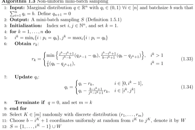
In Algorithm 1.3 we describe an approach that we used to generate a non-uniform mini-batch sampling of mini-batchsizeb from a given marginal distributionq. Without loss of gener-ality, we assume that the qi ∈(0,1)for i∈[n]are sorted from largest to smallest.

We now state several facts about Algorithm 1.3.

1. Algorithm 1.3 will terminate in at mostniterations. This is because the update rules forqi(which depend on rk at each iteration), ensure that at least oneqi will reduce to

become equal to someqj < qi (i.e., eitherqik+1₋₁=q_b orq_jk+1₊₁ =q_b) and since there

(32)

Algorithm 1.3 Non-uniform mini-batch sampling

1: Input: Marginal distribution q ∈_Rn _with_q

i ∈(0,1)∀i∈[n]and batchsize bsuch that

Pn

i=1qi =b. Defineqn+1 = 0

2: Output: A mini-batch samplingS (Definition 1.5.1)

3: Initialization: Index set i, j∈_Nn_{, and set}_k_{= 1}_.

4: fork= 1, . . . , ndo 5: ik= mini{i:pi =qb}, jk= maxi{i:pi =qb} 6: Obtain rk: rk= ( min n jk₋_ik₊₁ jk₋_b (qik₋₁−q_b),j k₋_ik₊₁ b−ik₊₁ (qb−qjk₊₁) o , ik >1 j b(qb−qjk₊₁), ik = 1 (1.33) 7: Update qi: qi= ( qi−rk, i∈[0, ik−1], qi− b−i k₊₁ jk₋_ik₊₁rk, i∈[ik, jk] (1.34)

8: Terminate if q= 0, and setm=k

9: end for

10: SelectK∈[m]randomly with discrete distribution(r1, . . . , rm)

11: Chooseb−iK+ 1coordinates uniformly at random fromiK to jK, denote it byW

12: S={1, . . . , iK−1} ∪W

i, j∈[n]. Note that if the algorithm begins withqi =qj for alli, j∈[n], which implies

a uniform marginal distribution, the algorithm will terminated in a single step.

2. For Algorithm 1.3 we must have Pm

i=1ri = 1, where we assume that the algorithm

terminates at iterationm∈[1, n], since overall we havePm

i=1bri =Pni=1qi=b.

3. Algorithm 1.3 will always generate a proper sampling because when it terminates, the situation pi =pj >0, for all i6=j, will always hold. Thus, any subset of size b has a

positive probability of being sampled.

4. It can be shown that this algorithm works on an arbitrary given marginal probabilities as long asqi ∈(0,1), for alli∈[n].

Figure 1.1 is a sample illustration of Algorithm 1.3, where we have a marginal distribution for 4 coordinates given by (0.8,0.6,0.4,0.2)T and we set the batchsize to beb = 2. Then, the algorithm is run and findsr to be(0.2,0.4,0.4)T. Afterwards, with probabilityr1= 0.2,

we will sample 2-coordinates from (1,2). With probability r2 = 0.4, we will sample 2

(33)

at random and with probability r3 = 0.4, we will sample 2-coordinates from (1,2,3,4)

uniformly at random.

Note that, here we only need to perform two kinds of operations. The first one is to sample a single coordinate from distribution d (see Section 1.5.1), and the second is to sample batches from a uniform distribution (see for example [74]).

r3=0.4 r2=0.4 r1=0.2 q1=0.8 q2=0.6 q3=0.4 q4=0.2 r3/2 r3/2 r3/2 r3/2 r2 r2/2 r2/2 r1 r1

Figure 1.1: Toy demo illustrating how to obtain a non-uniform mini-batch sampling with batch size b= 2 fromn= 4 coordinates.

1.5.3 Mini-batch adfSDCA algorithm

Here we describe a new adfSDCA algorithm that uses a mini-batch scheme. The algorithm is called mini-batch adfSDCA and is presented below as Algorithm 1.4.

Algorithm 1.4 Mini-Batch adfSDCA

1: Input: Data: {xi, φi}ni=1

2: Initialization: Choose α(0) ∈_Rn _{and set batchsize}_b

3: fort= 0,1,2, . . . do

4: Calculate dual residue κ(_it)=φ0_i(xT_i w(t)) +α(_it), for all i∈[n]

5: Generate the adaptive probability distribution p(t) ∼κ(t)

6: Choose mini-batchS ⊂[n]of sizebaccording to probabilities distributionp(t)

7: Set step-sizeθ(t)∈(0,1)as in (A.36) 8: fori∈S do 9: Update: α(_it+1) =α(_it)−θ(t)(bp(_it))−1κ(_it) 10: end for 11: Update: w(t+1)=w(t)−P i∈Sθ(t)(nλbp (t) i ) −1_κ(t) i xi 12: end for

Briefly, Algorithm 1.4 works as follows. At iteration t, adaptive probabilities are gener-ated in the same way as for Algorithm 1.1. Then, instead of updating only one coordinate, a mini-batch S of size b ≥ 1 is chosen that is consistent with the adaptive probabilities. Next, the dual variablesα(_it), i∈S are updated, and finally the primal variablewis updated according to the primal-dual relation (1.6).

(34)

In the next section we will provide a convergence guarantee for Algorithm 1.4. As was discussed in Section 1.3, theoretical results are detailed under two different assumptions on the type of loss function: (i) all loss function are convex; and (ii) individual loss functions may be non-convex but the average over all loss functions is convex.

1.5.4 Expected Separable Overapproximation

Here we make use of the Expected Separable Overapproximation (ESO) theory introduced in [74] and further extended, for example, in [72]. The ESO definition is stated below.

Definition 1.5.2 (Expected Separable Overapproximation, [72]). Let Sˆ be a sampling with

marginal distribution q = (q1,· · ·, qn)T. Then we say that the function f admits a v-ESO

with respect to the samplingSˆ if∀x, h∈_Rn_{, we have}_v

1, . . . , vn>0, such that the following

inequality holds _E[f(x+h_{[ ˆ}_S_])]≤f(x) +Pn

i=1qi(∇if(x)hi+ 1 2vih2i).

Remark 1.5.3. Note that, here we do not assume thatSˆis a uniform sampling, i.e., we do

not assume that qi =qj for all i, j∈[n].

The ESO inequality is useful in this chapter because the parametervplays an important role when setting a suitable stepsizeθ in our algorithm. Consequently, this also influences our complexity result, which depends on the sampling Sˆ. For the proof of Theorem 1.5.5 (which will be stated in next subsection), the following is useful. Letf(x) = 1₂kAxk2_{, where}

A= (x1, . . . , xn). We say that f(x) admits av-ESO if the following inequality holds

E[kAh_Sˆk2]≤

n

X

i=1

viqih2i. (1.35)

To derive the parameter v we will make use of the following theorem.

Theorem 1.5.4([72]). Letf satisfy the following assumptionf(x+h)≤f(x)+h∇f(x), hi+

1 2h

T_AT_AhT_, _where _A _{is some matrix. Then, for a given sampling} _S,_ˆ _f _{admits a} _v-ESO,

where v is defined by vi = min{λ0(P( ˆS)), λ0(ATA)}Pm_j₌₁A2_ji, i∈[n].

HereP( ˆS)is called a sampling matrix (see [74]) where elementpij is defined to bepij =

P

(35)

M, i.e., λ0(M) = maxkhk=1{hTM h : Pni=1Miih2i ≤ 1}. We may now apply Theorem 1.5.4

because f(x) = 1₂kAxk2 _{satisfies its assumption. Note that in our mini-batch setting, we}

have P_S_∈_Sˆ(|S| = b) = 1, so we obtain λ0(P( ˆS)) ≤ b (Theorem 4.1 in [72]). In terms of

λ0(ATA), note that λ0(ATA) =λ0(Pm

j=1xjxTj) ≤maxjλ0(xjxTj) = maxj|Jj|, where|Jj| is

number of non-zero elements of xj for each j. Then, a conservative choice from Theorem

1.5.4 that satisfies (1.35) is

v_i0 = min{b,max

j |Jj|}kxik

2_, _i_∈_[_n_]_. _(1.36)

Now we are ready to give our complexity result for mini-batch adfSDCA (Algorithm 1.4). Note that we use the same notation as that established in Section 1.3 and we also define Q0def= 1 n n X i=1 v0_i. (1.37)

Theorem 1.5.5. Let L,˜ κ(_it), γ D(t), v_i0, C0 and Q0 be as defined in (1.5), (1.7), (1.12),

(1.13), (1.36), (1.21) and (1.37), respectively. Suppose that φi is L-smooth and convex for

all i∈[n]. Then, at every iteration t≥0 of Algorithm 1.4, run with batchsize b we have

E[D(t+1)|α(t)]≤(1−θ∗)D(t), (1.38)

where θ∗ = Pn nλ2b

i=1(v

0

iγ+nλ2)

. Moreover, it follows that whenever

T ≥ n b + ˜ LQ0 bλ log (λ+ ˜L)C0 λL˜ , (1.39) we have that E[P(w(T)−P(w∗))]≤.

It is also possible to derive a complexity result in the case when theaverage of thenloss functions is convex. The theorem is stated now.

Theorem 1.5.6. Let L, κ(_it), γ¯ D¯(t), v_i0, C¯0 and Q0 be as defined in (1.5), (1.7), (1.26),

(1.27),(1.36), (1.28)and (1.37)respectively. Suppose that everyφi, i∈[n]isLi-smooth and

that the average of then loss functions 1_nPn

(36)

t≥0 of Algorithm 1.4, run with batchsize b, we have

E[ ¯D(t+1)|α(t)]≤(1−θ∗) ¯D(t), (1.40)

where θ∗ = Pn nλ2b

i=1(v0i¯γ+nλ2)

. Moreover, it follows that whenever

T ≥ n b + Q0_n1Pn i=1L2i bλ log (λ+ ˜L) ¯C0 ¯ γ , (1.41) we have that _E[P(w(T))−P(w∗)]≤.

These theorems show that in worst case (by setting b = 1), this mini-batch scheme shares the same complexity performance as the serial adfSDCA approach (recall Section 1.2). However, when the batch-size bis larger, Algorithm 1.4 converges in fewer iterations. This behavior will be confirmed computationally in the numerical results given in Section 1.6.

1.6

Numerical experiments

Here we present numerical experiments to demonstrate the practical performance of the adfSDCA algorithm. Throughout these experiments we used two loss functions, quadratic loss φi(wTxi) = 1₂(wTxi −yi)2 and logistic loss φi(wTxi) = log(1 + exp(−yiwTxi)). Note

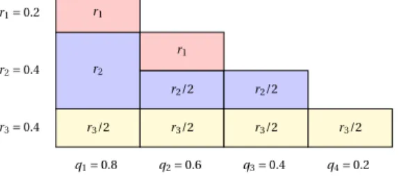
that these two losses have Lipschitz gradient. The regularization parameter λ in (1.1) is set to be 1/√n, where n is the number of samples of the dataset. The experiments were run using datasets from the standard library of test problems (see [11] and http:

//www.csie.ntu.edu.tw/~cjlin/libsvm), as summarized in Table 1.1.

Dataset #samples #features #classes sparsity

mushrooms 8,124 112 2 18.8%

ijcnn1 49,990 22 2 59.1%

rcv1 20,242 47,237 2 0.16%

news20 19,996 1,355,191 2 0.034%

(37)

1.6.1 Comparison for a variety of adfSDCA approaches

In this section we compare the adfSDCA algorithm (Algorithm 1.1) with both dfSCDA, which is a uniform variant of adfSDCA described in [83], and also with Prox-SDCA from [87]. We also report results using Algorithm 1.2, which is a heuristic version of adfSDCA, used with several different shrinkage parameters.

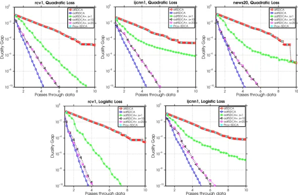
Figure 1.2 compares the evolution of the duality gap for the standard and heuristic variant of our adfSDCA algorithm with the two state-of-the-art algorithms dfSDCA and Prox-SDCA. For these problems both our algorithm variants out-perform the dfSDCA and Prox-SDCA algorithms. Note that this is consistent with our convergence analysis (recall Section 1.3). Now consider the adfSDCA+algorithm, which was tested using the parameter values s = 1,10,20. It is clear that adfSDCA+ with s = 1 shows the worst performance, which is reasonable because in this case the algorithm only updates the sampling probabili-ties after each epoch; it is still better than dfSDCA since it utilizes the sub-optimality at the beginning of each epoch. On the other hand, there does not appear to be an obvious differ-ence between adfSDCA+used withs= 10ors= 20with both variants performing similarly. We see that adfSDCA performs the best overall in terms of the number of passes through the data. However, in practice, even though adfSDCA+ may need more passes through the data to obtain the same sub-optimality as adfSDCA, it requires less computational effort than adfSDCA.

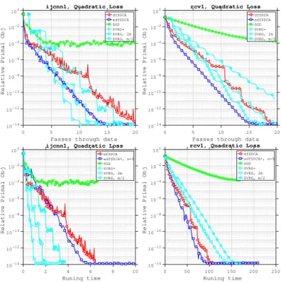
In Figure 1.3, we compare SGD, SVRG, dfSDCA and our proposed adfSDCA(+) al-gorithm in terms of the number of passes through the data and total running time. For the SGD and SVRG algorithms, the duality gap is not directly computable. Hence, in this numerical experiment, the relative primal objective valueP(w)−P( ˆw) is used as the stop-ping condition, where wˆ is the optimal weight given by the best run among all algorithms. The SGD algorithm is implemented using the same set-up as in [85], where a diminishing step-size is used, and SVRG is implemented following [36].

We remark that for the SVRG algorithm, the user must tune its two hyper-parameters, namely, the number of iterations in the inner loop, and the step-size. Proper tuning of these hyper-parameters is essential to get the best performance from the SVRG algorithm. In this

(38)

2 4 6 8 10 10−10 10−8 10−6 10−4 10−2 100 rcv1, Quadratic Loss

Passes through data

Duality Gap dfSDCA adfSDCA adfSDCA+, s=1 adfSDCA+, s=10 adfSDCA+, s=20 Prox−SDCA 2 4 6 8 10 10−10 10−8 10−6 10−4 10−2 100

ijcnn1, Quadratic Loss

Passes through data

news20, Quadratic Loss

Passes through data

Duality Gap dfSDCA adfSDCA adfSDCA+, s=1 adfSDCA+, s=10 adfSDCA+, s=20 Prox−SDCA 2 4 6 8 10 10−10 10−8 10−6 10−4 10−2 100 rcv1, Logistic Loss

Passes through data

ijcnn1, Logistic Loss

Passes through data

Duality Gap dfSDCA adfSDCA adfSDCA+, s=1 adfSDCA+, s=10 adfSDCA+, s=20 Prox−SDCA

Figure 1.2: A comparison of the number of epochs versus the duality gap for the various algorithms.

experiment, we tuned the hyper-parameters for SVRG, and we used SVRG+ to denote the best performing SVRG variant, and we usemto denote the corresponding ‘best’ number of inner loop iterations. As a means of comparison, we also plot the performance of the SVRG algorithm using m/2 and 2minner loop iterations (i.e., SVRG without optimal tuning).

Figure 1.3 shows that, for the rcv1 dataset with a quadratic loss, adfSDCA is the best performing algorithm in terms of the number of passes through the data; it is even better than the ‘best’ tuned SVRG algorithm. For the ijcnn1 dataset with a quadratic loss, SVRG+, the optimally tuned SVRG algorithm, performs better than the adfSDCA algorithm. However, tuning the hyper-parameters for SVRG is not free, and this is a com-putational cost that is not required for adfSDCA. This highlights one of the benefits of adfSDCA, which does not require parameter tuning, and the specific step-size needed is given explicitly in Theorem 1.3.1.

We also present plots showing the total running time for these algorithms. We follow the set up in [13], and present the running time results using the heuristic algorithm adfSDCA+ with the shrinkage parameter set to s = 5(see Section 1.4). Recall that the rcv1 dataset

(39)

0 5 10 15 20 Passes through data

10-14 10-12 10-10 10-8 10-6 10-4 10-2 100

Relative Primal Obj

ijcnn1, Quadratic Loss

dfSDCA adfSDCA SGD SVRG+ SVRG, 2m SVRG, m/2 0 5 10 15 20

Passes through data

10-14 10-12 10-10 10-8 10-6 10-4 10-2 100

Relative Primal Obj

rcv1, Quadratic Loss dfSDCA adfSDCA SGD SVRG+ SVRG, 2m SVRG, m/2 0 2 4 6 8 10 Runing time 10-14 10-12 10-10 10-8 10-6 10-4 10-2 100

Relative Primal Obj

ijcnn1, Quadratic Loss

dfSDCA adfSDCA+, s=5 SGD SVRG+ SVRG, 2m SVRG, m/2 0 50 100 150 200 250 Runing time 10-14 10-12 10-10 10-8 10-6 10-4 10-2 100

Relative Primal Obj

rcv1, Quadratic Loss dfSDCA adfSDCA+, s=5 SGD SVRG+ SVRG, 2m SVRG, m/2

Figure 1.3: A comparison of the number of epochs versus the relative primal object value for SGD, dfSDCA, adfSDCA(+) and SVRG. SVRG+ denotes the parameter-tuned, best performing SVRG algorithm, where m denotes the corresponding number of inner loop iterations. We also show results for the SVRG agorithm using bothm/2 and2m inner loop iterations, to demonstrate the performance of SVRG without optimal tuning.

has n = 20,242 and d = 47,237, so the number of samples is comparable to the number of features. For this experiment, Figure 1.3 shows that the total running time needed for adfSDCA+ is much less than SVRG. However, for the ijcnn1dataset, SVRG outperforms adfSDCA+ in terms of running time. To gain some insight into why this is happening, recall that the ijcnn1 dataset has n = 49,990 and d = 22, so the number of samples is much more than the number of features. Note that adfSDCA+ must compute the residuals for each coordinate at every iteration, and because the number of samples is far greater than the number of feature, there is a high running time overhead for this non-uniform sampling of coordinates for adfSDCA+. This suggests that it is beneficial to use adfSDCA when the number of features is comparable with the number of samples.

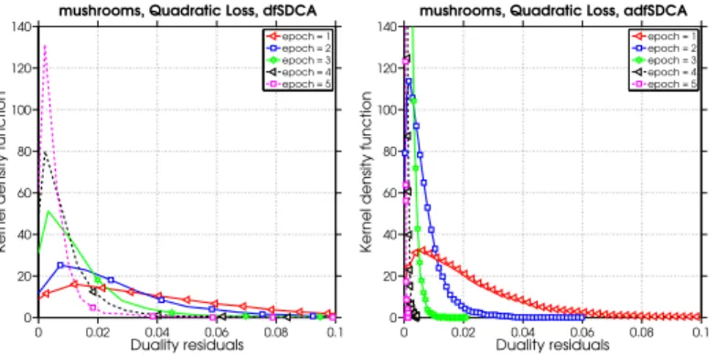
Figure 1.4 shows the estimated density function of the dual residue |κ(t)| after1,2,3,4

and 5 epochs for both uniform dfSDCA and our adaptive adfSDCA. One observes that the adaptive scheme is pushing the large residuals towards zero much faster than uniform

(40)

dfSDCA. For example, notice that after 2 epochs, almost all residuals are below 0.03 for adfSDCA, whereas for uniform dfSDCA there are still many residuals larger than0.06. This is evidence that, by using adaptive probabilities we are able to update the coordinate with a high dual residue more often and therefore reduce the sub-optimality much more efficiently.

0 0.02 0.04 0.06 0.08 0.1 0 20 40 60 80 100 120 140

mushrooms, Quadratic Loss, dfSDCA

Duality residuals

Kernel density function

epoch = 1 epoch = 2 epoch = 3 epoch = 4 epoch = 5 0 0.02 0.04 0.06 0.08 0.1 0 20 40 60 80 100 120 140

mushrooms, Quadratic Loss, adfSDCA

Duality residuals

Kernel density function

epoch = 1 epoch = 2 epoch = 3 epoch = 4 epoch = 5

Figure 1.4: Comparing absolute value of dual residuals at each epoch between dfSDCA and adfSDCA.

1.6.2 Mini-batch adfSDCA

Here we investigate the behavior of the mini-batch adfSDCA algorithm (Algorithm 1.4). In particular, we compare the practical performance of mini-batch adfSDCA using different mini-batch sizesbvarying from1to 32. Note that ifb= 1, then Algorithm 1.4 is equivalent to the adfSDCA algorithm (Algorithm 1.1). Figures 1.5 shows that, with respect to the different batch sizes, the mini-batch algorithm with each batch size needs roughly the same number of passes through the data to achieve the same sub-optimality. However, when considering the computational time, the larger the batch size is, the faster the convergence will be. Recall that the results in Section 1.5 show that the number of iterations needed by Algorithm 1.4 used with a batch size ofbis roughly1/btimes the number of iterations needed by adfSDCA. Here we compute the adaptive probabilities every b samples, which leads to roughly the same number of passes through the data to achieve the same sub-optimality.

(41)

0 2 4 6 8 10 10−8 10−6 10−4 10−2 100

Passes through data

Duality Gap b = 1 (adfSDCA) b = 2 b = 4 b = 8 b = 16 b = 32 0 100 200 300 400 10−8 10−6 10−4 10−2 100

Runing time Duality Gap b = 1 (adfSDCA) b = 2 b = 4 b = 8 b = 16 b = 32 0 2 4 6 8 10 10−8 10−6 10−4 10−2 100 rcv1, Logistic Loss

Passes through data

Duality Gap b = 1 (adfSDCA) b = 2 b = 4 b = 8 b = 16 b = 32 0 50 100 150 200 250 300 10−12 10−10 10−8 10−6 10−4 10−2 100 rcv1, Logistic Loss Runing time Duality Gap b = 1 (adfSDCA) b = 2 b = 4 b = 8 b = 16 b = 32

Figure 1.5: Comparing the number of iterations of various batch size on different losses.

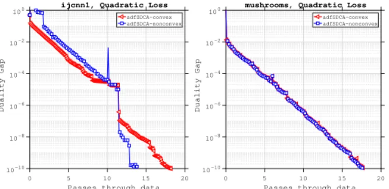
1.6.3 adfSDCA for non-convex loss

Here we investigate the behavior of adfSDCA when applied to problems that involve some nonconvex loss functions. We describe the experimental set-up now. Suppose that we have convex loss functions φi(xTi w), where i∈ [n]. Then, it is possible to construct nonconvex

loss functions by subtracting a quadratic from each of the convex losses as follows:

¯

φi(xTi w) =φi(xTi w)−Cikwk2. (1.42)

Note that if Ci >0 is large enough (up to the Lipschitz gradient constant of φi(xTi w)), the

new lossφ¯i(xT_iw)derived by (1.42) will be nonconvex. On the other hand, ifCi <0, we will

have the new loss being strongly convex.

Now, functions of the form (1.42) will satisfy the requirements of Case II in Section 3.2 (i.e., that the individual loss functions can be nonconvex, but that the average over all the losses is convex) as long as some of the hyperparametersCi are large enough to make (1.42)

nonconvex andPn

i=1Ci= 0. Using this set-up, we present a numerical experiment to show

(42)

due to that the new loss (1.42) would be nonconvex when Ci > 0, since the Hessian of

each quadratic loss of xi has the smallest eigenvalue 0. In particular, we let Ci = 0.01×

(−1)i, where i∈ [n]. We use themushrooms and ijcnn1 datasets for this experiment, and because these datasets both have an even number of samples, the property thatPn

i=1Ci = 0

will hold. The results of this experiment are shown in Figure 8, where we compare the performance of adfSDCA with respect to the running time and number of passes over the data. Figure 8 shows that adfSDCA performs well on such problems and is able to find an accurate solution (where the duality gap is less than 10−10) in less than20 passes over the data.

0 5 10 15 20

Passes through data 10-10 10-8 10-6 10-4 10-2 100 Duality Gap

ijcnn1, Quadratic Loss adfSDCA-convex adfSDCA-nonconvex

0 5 10 15 20

Passes through data 10-10 10-8 10-6 10-4 10-2 100 Duality Gap

mushrooms, Quadratic Loss

adfSDCA-convex adfSDCA-nonconvex

Figure 1.6: Comparing adfSDCA for two cases on quadratic loss.

1.7

Conclusion

In this chapter, we present dual free SDCA variants with adaptive probabilities for Empir-ical Risk Minimization problems. The theoretEmpir-ical complexity of the proposed methods is analyzed in two cases: when the individual loss functions are all convex and when the av-erage over the losses is convex but individual loss functions may be nonconvex. A heuristic variant of adfSDCA is proposed to reduce the computational effort required and its practical convergence performance is demonstrated via a numerical experiment. We also extend our convergence theory to cover a mini-batch adfSDCA variant and a novel nonuniform sampling strategy for mini-batches is developed. Our experimental results show speedups in terms of the number of passes through the data and/or running time of the proposed methods, when compared with the original dual free SDCA, as well as other state-of-art primal methods.

(43)

The numerical experiments related to the use of mini-batches match our theoretical analysis and suggest that using mini-batches is beneficial in practice.

Acknowledgement

We would like to thank Professor Alexander L. Stolyar for his insightful help with Algo-rithm 1.3.

(44)

Chapter 2

Large-scale Distributed Hessian-Free

Optimization for Deep Neural

Networks

2.1

Introduction

Deep learning has shown great success in many practical applications, such as image classi-fication [43, 89, 27], speech recognition [31, 81, 1], etc. Stochastic gradient descent (SGD), as one of the most well-developed method for training neural network, has been widely used. Besides, there has been plenty of interests in second order methods for training deep networks [51]. The reasons behind these interests are multi-fold. At first, it is generally more substantial to apply weight updates derived from second order methods in terms of optimization aspect, meanwhile, it takes roughly the same time to obtain curvature-vector products [39] as it takes to compute gradient which make it possible to use second order method on large scale model. Furthermore, computing gradient and curvature information on large batch (even whole dataset) can be easily distributed across several nodes. Recent work has also been used to reveal the significance of identifying and escaping saddle point by second order method, which helps prevent the dramatic deceleration of training speed around the saddle point [17].

(45)

Line search Newton-CG method (also known as the truncated Newton Method), as one of the practical techniques to achieve second order method on high dimensional optimization, has been studied for decades [65]. Recent work to apply Newton-CG method has been proved as a practical and successful achievement on training deep neural network[51, 39]. Indeed, for Newton-CG method, at each iteration, an approximated Hessian matrix is constructed, and naïve conjugate gradient (CG) method is applied to obtain a descent direction. The naïve CG method is, however, designed to solve positive definite systems, i.e., it requires the approximate Hessian matrix to be positive definite. Otherwise, the CG iteration is terminated as soon as a negative curvature direction is generated. Note that Newton-CG method does not require explicit knowledge of Hessian matrix, and it requires only the Hessian-vector product for any given vector. One special case for using Hessian-vector product is to train deep neural network, also known as Hessian-free optimization, and such Hessian-free optimization is exactly used in Marten’s HF [51] methods.

As discussed in [17], identifying and escaping saddle points significantly improve training performance. This implies the necessity to use negative curvature direction. Conventionally with Newton-CG methods, the negative curvature direction is simply ignored, which may lead to unsatisfactory training. In this chapter, we highlight the importance of the using of negative curvature direction and the its impact therein on training, with a small demo example. we go to further derive ways to find negative curvature direction and propose a novel algorithm to use such negative curvature effectively.

Moreover, it is well known that traditional SGD method is inherently sequential and be-comes very expensive (time-to-train) to apply on very large data sets. More detail discussion can be found in [102], wherein Momentum SGD (MSGD) [92], ASGD and MVASGD [70], are considered as alternatives. However, it is shown that these methods have limited scaling potential, due to the limited concurrency. However, unlike SGD, Hessian-free methods (in this work, we are focus on full gradient and stochastic Hessian-vector product evaluation) can be distributed naturally, allow for large mini-batch sizes (increased parallelism) while improving convergence rate and also the better the quality of