Automatic Detection of Optic Disc in Digital Retinal
Images
Kittipol Wisaeng
Computer Science Department of Computer Science, King Mongkut's Institute of Technology
Ladkrabang, Thailand
Nualsawat Hiransakolwong
Computer Science Department of Computer Science, King Mongkut's Institute of Technology
Ladkrabang, Thailand
Ekkarat Pothiruk
Ophthalmology Unit Khonkean Hospital,
Khonkean, Thailand
ABSTRACT
On the research work leading to automatic detection of optic disc from retinal images is very essential and crucial for expert ophthalmologists to diagnose diseases. Many of techniques can achieve good performance on retinal feature that is clearly visible. Unfortunately, it is a normal situation that the color retinal images in Thailand are poor-quality images. The existing algorithm cannot detected poor-quality images. Therefore, this study is a part of larger efforts to develop a novel method for detection of optic disc in poor-quality retinal images. A novel method is presented towards the development for detection of optic disc in poor-quality retinal images. The digital retinal images are detected by using morphological method and Otsu’s algorithm after the key preprocessing steps, i.e., color normalization, contrast enhancement and noise removal. This enables the difference in the proposed method compared to other approaches and the algorithm can achieve good performance even on poor-quality retinal images. The proposed method was evaluated using the local dataset and the publicly available of the STARE project’s dataset. The optic disc was detected correctly in 91.35% using the STARE dataset and 97.61% using the local dataset. This system intends to help expert ophthalmologists in screening process to detect of optic disc faster and more easily.
General Terms
Medical Image ProcessingKeywords
Optic Disc, Morphological Method, Otsu’s Methods, STARE Databases, Expert Ophthalmologists
1.
INTRODUCTION
The optic disc is considered one of the main features of a retinal image (Fig. 1), where methods are described for its automatic detection. The detection of optic disc is a key pre-processing component in many algorithms designed for the automatic extraction of retinal anatomical structures and lesions. Unfortunately, in a normal situation, digital retinal images in Thailand are poor-quality images. The detection of optic disc in poor-quality images is difficult; taking a long processing time and the expensive computational cost becoming a bottleneck that limits clinical application. Some methods estimated the boundary of the optic disc as a circle or an ellipse [1], [2], [3], [4]. Other methods have been proposed for the exact detection of the optic disc contour, e.g., snakes [5], pyramidal decomposition [6] and a Hausdorff-based template matching [7], gradient vector flow [8], which largely have the ability to bridge discontinuities of the edges.
However, these algorithms often fail for poor quality retinal images with a large dataset.
After starting the motivations of localized the optic disc, defining the optic disc and highlighting the difference between disc detection and disc boundary detection, the remaining part of the study is organized as follows. In Section 2, a description of the used material is given. Section 3, presents the proposed algorithm. The experimental results are presented in Sections 4. Finally, conclusions of the article are found in Section 5.
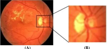
(A) (B)
Fig 1: (A) Typical image (B) Optic disc close-up view
2.
MATERIALS AND METHODS
2.1
Patients
[image:1.595.315.542.353.457.2]2.2 Data Preparation
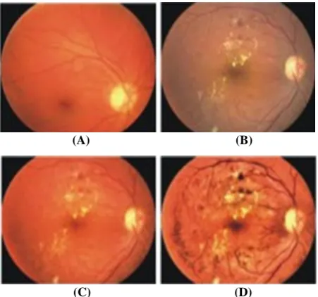
[image:2.595.55.282.123.383.2]Typically, there is wide variation in the color of retinal images from different patients that are strongly correlated to person’s race and iris colors (Fig. 3).
Fig. 2. The outline of ours the proposed system for automatic detection of optic disc
(A) (B)
Fig. 3. (A) and (B) Example of poor quality retinal images
Hence, we put our retinal images through four pre-processing steps before commencing the detection of optic disc. The first step is to color normalize the color of the retinal images across the dataset. We selected a retinal image as a reference (the image was chosen in agreement with the expert ophthalmologist) and then applied histogram specification [9] to modify the value of each image in the dataset. After the procedure of normalization, the contrast of retinal images was not sufficient due to the intrinsic attributes of optic disc and decreasing color saturation, especially in the periphery. Consequently, in the second preprocessing step, the contrast between the optic disc and the retina background was enhanced to facilitate later detection. We applied local contrast enhancement to distribute the values of pixels around the local mean [10].
Consider a sub-image W of the size M×M pixels centered on a pixel. Let mean and standard deviation of the intensity within W be <f>W and σW respectively. Also denotes fmax and fmin as the maximum and minimum intensities of the whole image. Then the adaptive local contrast enhancement transformation is defined by Eq. (1).
W W min
W max W min Ψ (f)-Ψ (f ) g(x, y) = 255
Ψ (f ) - Ψ (f )
(1)
where, the sigmoidal function w is defined by Eq. (2).
1 W
W
W (f ) f (x, y) 1 exp
(2)
And fmax and fmin are the maximum and minimum intensity values in the whole image, while <f>w and σw indicate the
local window mean and standard deviation which are defined as Eq. (3).
w 2
(i, j) w (k,l)
1
f
f (i, j)
M
(3)2
w 2 w
(i, j)w (k,l)
1
(f (i, j)
f
)
M
(4)where, (x, y) represents the location of each pixel within window w. The size of window M should be chosen to be large enough to contain a statistically representative distribution of the local variations of pixels. The exponential function (Eq. (2) produces significant enhancement when the contrast is low (σw is small), while it provides less enhancement if the contrast is already high (σw is large)). While the contrast enhancement improves the contrast of optic disc it also enhances the contrast of some artifact (e.g., noise). Therefore, these pixels may wrongly be detected as optic disc. There are several ways to remove or reduce noise in an image. We found the median filtering is better able to remove these outliers without reducing the sharpness of the image [11]. The benefit of median filter is simultaneously reducing noise and preserving edges. Therefore, a median filtering operation is applied on the intensity band in third preprocessing step. Finally, Red, Green and Blue (RGB) space of original retinal image is transformed to Luv color space. The result of all preprocessing step is illustrated in Fig. 4.
(A) (B)
(C) (D)
Fig. 4. Color normalization and contrast enhancement results; (A) the reference images, (B) poor quality retinal
image, (C) the color normalized version of (B), (D) contrast enhanced version of (C), modified from []
2.3 Optic Disc Detection
[image:2.595.316.542.402.613.2]cup. In either case the cup appears as a smaller, brighter region within the optic disc. Whereas locating the optic disc is an apparently simple task for as expert to trace the boundary, traditional general-purpose boundary detection algorithms have not fully succeeded in detecting the optic disc due to fuzzy boundaries, inconsistent image contrast, variability in appearance or missing edge features. Therefore, a reliable optic disc localization is difficult. Some of example difficult in optic disc localization is illustrated in Fig. 5.
Fig. 5. Optic disc and optic cup in retinal image
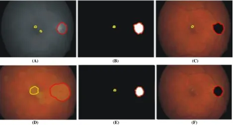
Consequently, in order to effectively detect the optic disc, in this study two techniques are combination of morphology methods and Otsu’s algorithms are presented. The morphological methods generally work by two images and a structuring element (instead of a single image and structuring element). One image, the marker, is the starting point for the transformation. The other image, the mask, constrains the transformation. This task is made extremely difficult since the optic disc region is fragmented into multiple sub regions by blood vessels.
Furthermore, the blood vessels enter the optic disc from different directions with a general tendency to concentrate
around the nasal side of the optic disc region [12]. Therefore, in the first stage, we used morphological closing for gray scale images on the intensity channel to remove and closing the blood vessels to create a fairly constant optic disc region. This stage, a structuring element (SE = strel(‘disk’, R)) creates a flat, disk-shaped structuring element, where R specifies the radius. R must be a non-negative integer such as 0, 4, 6, or 8. In this work, a flat structuring element 8 is used. The result of closing for gray scale images on the intensity image is illustrated in Fig. 6A. It is evident that this approach produces a more homogeneous region while preserving the optic disc edges. The examples above illustrate the use of gray-scale reconstruction in optic disc analysis tasks. However, it is probably for binary segmentation that this operation is most useful. Therefore, in the second stage, a global image threshold using Otsu’s method is used to convert an intensity image to a binary image, separating brighter regions from dark background. A global threshold (level=graythresh (image_close)) that can be used to convert an intensity image to a binary image with im2bw(image_close, level) is a normalized intensity value that lies in the range [0, 1]. The graythresh function uses Otsu’s method, which chooses the threshold to minimize the intraclass variance of the black and white pixels. This stage, intensity with a fixed value with 0.7 is used. The result of retinal image is binarized with thresholding is show in Fig. 6B. Afterward, all pixel from Fig. 6B is used as mask and they were overlaid on the original images to candidate optic disc regions. An example of the maker images is shown in
Fig. 6C. Consider from Fig. 6D, imdilate image was applied on the previously overlaid image. The argument of a structuring element object, or array of structuring element objects, returned by the strel function. This stage, structuring element with a fixed value with 5 is used. In the fourth stage, convert image to binary image, based on threshold (image_threshold2) with im2bw (image_Luv-op3).
The output image BW replaces all pixels in the input image with luminance greater than level with the value 1 (exudates
(A) (B) (C)
(D) (E) (F)
[image:3.595.64.535.476.728.2]pixels) and replaces all other pixels with the value 0 (background pixels). Specify level in the range [0, 1]. In this stage, a level value of 0.70 is used separating between exudates and background. The resulting retinal image is binarized with thresholding is show in Fig. 6E. As a result, high intensities are reconstructed while the rest is removed.
Pseudo Code 1 is the algorithm for the optic disc boundary detection.
Pseudo Code 1: Optic Disc Boundary Detection Inputs: Image_rgb = imfile; %imread(imfile)
image_Luv = rgb2luv(image_rgb); Output: 1. se = strel(‘disk’, 8);
image_close = imclose(image_luv(:,:,3), se); level = graythresh(image_close)+0.21; image_threshold = im2bw(image_close, level);%image_gray>=0.70;
2. OP2 = image_luv; OP2_1 = op2(:,:,1); OP2_2 = op2(:,:,2); OP2_3 = op2(:,:,3);
OP2_1(find(image_threshold==1)) =0; OP2_2(find(image_threshold==1)) =0; OP2_3(find(image_threshold==1)) =0; OP2 = cat(3,op2_1,op2_2,op2_3); 3. se2 = strel(‘disk’, 5);
OP3 = imdilate(op2, se2); while numel(find(op3==0)) > 0 OP3 = imdilate(op3, se2); end
4. level2 = graythresh(op3);
image_threshold2 = im2bw(image_luv-op3, 0.01); %image_gray>=0.70;
OP4 = image_threshold2; %image_luv-op3;
Typically, the optic disc can be seen brighter than the surrounding area. Despite its brightness, an accurate localization is not an easy task as some part are obscured by crossing blood vessels and in some case, such as the affected of bright the lesions. However, the shape of optic disc is round; therefore the optic disc region selection process needs to be made specific to the largest one among the regions and compactness whose shapes are circular by using Pseudo Code 2.
Pseudo Code 2: Optic Disc Localization Inputs: OP4 (Optic Disc4)
Output: 1. maxGroup = max(L(:)); M = zeros(1, maxGroup); for i=1:maxGroup [r, c] = find(L==i); rc = [r c];
max_r = abs(r(1)-r(end)); max_c = abs(c(1)-c(end)); if (max_r < max_c) radius = max_r; else
radius = max_c; end
area = numel(rc); if (area>3000)
region border= 2*pi*(radius/2);
mm = 4*pi*(area/(region border * region border)); M(i) = abs(area-mm);
else
M(i) = inf; end
end
2. se3 = strel(‘disk’, 7); LL = imdilate(LL, se3); while numel(find(LL==0)) > 0 LL = imdilate(LL, se3); end
3. OP5 = origin; OP5_1 = op5(:,:,1); OP5_2 = op5(:,:,2); OP5_3 = op5(:,:,3); OP5_1(find(L==cc(1))) =0; OP5_2(find(L==cc(1))) =0; OP_3(find(L==cc(1))) =0;
From Pseudo Code 2, maxGroup = max(L(:)) returns the largest elements along different dimensions of an array. L is a vector, max(L) returns the largest element in L. M = max(L,[],dim) returns the largest elements along the dimension of L specified by scalar dim. For example, max_r = absolute (r, [1],-r) produces the maximum values along the first dimension of L while max_c = absolute (c,[1],-c) produces the maximum values along the second dimension of L. If max_r less than max_c, the radius of the conducting in max_r. The area is the number of pixels in the region while region border is the total number of pixel around the boundary of each region. If area more than 3000 pixels, the maxgroup of optic disc regions is calculated by Eq. (5) and the result is illustrated in Fig. 6F.
2 4 (area) max Group
(region border)
(5)
3. RESULTS
The retinal image with varying shapes, size and location of optic disc were used in this process. The resulting segmentation is compared against manually labeled ground-truth produced by an expert ophthalmologist and the final contour to illustrate the close match achieved. Fig. 7 shows a satisfactory detection for a circular shaped optic disc. We quantify the accuracy of the boundary localization against the manually labeled ground-truth produced by expert. We use a simple and effective overlap measure of the between two regions by using Eq. (6).
n(R T)
M 100
n(R)
(6)
(A) (B) (C)
Fig. 7. Optic disc boundary extraction results (A) hand-labeled (B) final contour (C) overlay of (A) and (B)
4. CONCLUSION AND DISCUSSION
We have shown several work retinal image analysis. We dealt with the problem of non-uniform illumination and poor contrast in color retinal images. The pre-processing stage showed remarkable gain in contrast enhancement related to retinal structures against background. The background exhibited a much more uniform illumination distribution. Weintroduce a different algorithm for detection of optic disc by mathematical morphology and Otsu’s algorithm. The algorithm yielded a fair approximation to the actual hand-labeled optic disc. The accuracy result is quite successful with accuracy of 91.35% compared to accuracy of the STARE dataset and achieved better results compared to the reviewed methods. In addition, the accuracy result is successful with accuracy of 97.61% compared to accuracy of the local dataset.
The speed of algorithm is approximately 34 sec (for one image). One visible advantage of this method is that the optic disc is detected even though the boundary of the optic disc is not continuous, blurred and different location. The system can be used even on a very poor computer system, such as those that may be available in rural area in developing countries
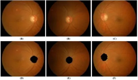
(B) (B) (C)
[image:5.595.58.536.183.460.2](D) (E) (F)
Fig. 8. The effect of rotation on one sample retinal image (A), (B) and (C) a typical retinal image (D), (E) and (F) optic disc area localized version of (A), (B) and (C), respectively
Table 1. The OD detection result for our proposed and literature reviewed methods
Author Method Local dataset (%) STAREdataset (%)
Sinthanayothin [1] Highest average variation 99.10 42.00
Lalonde [4] Hausdorff-based template matching 100.00 71.60
Li and Chutatape [5] Brightness guided 99.00 -
Haar [6] Resolution pyramid using a simple Haar-based 89.00 70.40
Osareh et al. [8] Averaged optic disc-images 100.00 58.00
Walter and Klein [13] Largest brightest connected object 100.00 58.00
Chrastek et al. [14] Highest average intensity 97.30 -
Barrett et al. [15] Hough transform as implemented by frank ter haar - 59.30
Hoover [16] Fuzzy convergence - 89.00
Lowell et al. [17] OD laplacian of gaussian 99.00 -
Tobin et al. [18] Vasculature-related OD 81.00 -
Abramoff and Niemeijer [19] Vasculature related OD properties and a kNN regression 99.90 -
[image:5.595.63.536.517.670.2]where both ophthalmologists and high performance computers are rarely available.
5. ACKNOWLEDGMENTS
This study was supported by the Commission on Higher Education, Mahasahakham University and in a part by King Mongkut's Institute of Technology Ladkrabang. We also would like to thank Mahasarakham Hospital for the retinal image used in this experiment.
6. REFERENCES
[1] Sinthanayothin, C., 1998. Automated localization of the optic disc, fovea and retinal blood vessels from digital colour fundus images. Br. J. Ophthalmol., pp: 902-910. PMID: 10413690
[2] Gagnon, L., Marc, L., Marie-Carole, B. 2001. Procedure to detect anatomical structures in optical fundus images. Processing of the Conference on Medical Image, (MI 01), San Diego, pp: 1218-1225. DOI: 10.1117/12.430999 [3] Abdel-Ghafar, R. A., 2004. Detection and characterization of the optic disc in glaucoma and diabetic retinopathy. Proceedings of the Medical Image Understanding Analysis Conference, (AC ‘04), London, UK, pp: 23-24.
[4] Lalonde, M. 2001. Fast and robust optic disc detection using pyramidal decomposition and Hausdorff-based template matching. IEEE Trans. Med. Imaging, PMID: 11700746
[5] Li, H., Chutatape, O. 2003. A model-based approach for automated feature extraction in fundus images. Proceedings of the 9th IEEE International Conference on Computer Vision, (CV ‘03), IEEE Computer Society. pp: 394-399. DOI: 10.1109/ICCV.2003.1238371
[6] Haar, T. F. 2005. Automatic localization of the optic disc in digital color images of human retinal. Utrecht University.
[7] Xu, C., 1997. Gradient vector flow: A new external force for snakes. Proceeding of the IEEE Conference on Computer Vision Pattern Recognition, Jun. 17-19, IEEE Xplore Press, San Juan, pp: 66-71. DOI: 10.1109/CVPR.1997.609299
[8] Osareh, A., Mirmehdi, M., Thomas, B., Markham, R. 2002. Classification and localisation of diabetic-related eye disease. Proceeding of the 7th European Conference on Computer Vision Copenhagen, Vision, May 28-31, Denmark, pp: 502-516. DOI: 10.1007/3-540-47979-1_34S
[9] Sinthanayothin, C., 1999. Image analysis for automatic diagnosis of diabetic retinopathy, Ph.D. Dissertation, UK.
[10]Meenalosini, S., Janet, J., Kannan, E. 2012. A novel approach in malignancy detection of computer aided diagnosis. Am. J. Applied Sci., 9: 1020-1029. DOI: 10.3844/ajassp.2012.1020.1029
[11]Osareh, A. 2009. Retinal markers for early detection of eye disease, automated image detection of retinal pathology. DOI: 10.1201/9781420037005.ch5
[12]Andres, G., Millán, M. S. 2011. Retinal image analysis: Preprocessing and feature extraction. J. Physics, 274: 1-8. DOI: 10.1088/17426596/274/1/012039
[13]Walter, T., Klein, J. C. 2001. Segmentation of color fundus images of the human retina: Detection of the optic disc and vascular tree using morphological techniques. Proceedings of the 2nd International Symposium on Medical Data Analysis, Oct. 8-9, pp: 282-287. DOI: 10.1007/3-540-45497-7_43
[14]Chrastek, R., Matthias, W., Klaus, D., Georg, M., Heinrich, N. 2002. Optic disc segmentation in retinal images. Bildverarbeitung Fur Die Medizin, pp. 263-266. DOI: 10.1007/978-3-642-55983-9_60
[15]Barrett, S. F., Naess, E., Molvik, T. 2001. Employing the hough transform to locate the optic disk. Biomed. Sci. Instrum., PMID: 11347450
[16]Hoover, A. 1998. Fuzzy convergence. Proceeding of the Conference Computer Vision and Pattern Recognition, Jun. 23-25, IEEE Xplore Press, Santa Barbara, pp: 716-721. DOI: 10.1109/CVPR.1998.698682
[17]Lowell, J., Hunter, A., Steel, D., Basu, A. 2004. Optic nerve head segmentation. IEEE Trans. Med. Image, 23: 256-264. DOI: 10.1109/TMI.2003.823261
[18]Tobin, K. W., Tobin, J. R., Chaum, E., Govindasamy, V.P., Karnowski, T. P., 2006. Characterization of the optic disc in retinal imagery using a probabilistic approach. Med. Image, 6144: 1088-1097. DOI: 10.1117/12.641670