ScholarWorks @ Georgia State University
ScholarWorks @ Georgia State University
Biology Dissertations Department of Biology
Summer 8-5-2012
Development of a Novel Method for Biochemical Systems
Development of a Novel Method for Biochemical Systems
Simulation: Incorporation of Stochasticity in a Deterministic
Simulation: Incorporation of Stochasticity in a Deterministic
Framework
Framework
Amit Sabnis
Georgia State University
Follow this and additional works at: https://scholarworks.gsu.edu/biology_diss
Recommended Citation Recommended Citation
Sabnis, Amit, "Development of a Novel Method for Biochemical Systems Simulation: Incorporation of Stochasticity in a Deterministic Framework." Dissertation, Georgia State University, 2012.
https://scholarworks.gsu.edu/biology_diss/120
INCORPORATION OF STOCHASTICITY IN A DETERMINISTIC FRAMEWORK
by
AMIT SABNIS
Under the Direction of Robert W. Harrison
ABSTRACT
Heart disease, cancer, diabetes and other complex diseases account for more than half of
human mortality in the United States. Other diseases such as AIDS, asthma, Parkinson’s disease,
Alzheimer’s disease and cerebrovascular ailments such as stroke not only augment this mortality
but also severely deteriorate the quality of human life experience. In spite of enormous financial
support and global scientific effort over an extended period of time to combat the challenges
posed by these ailments, we find ourselves short of sighting a cure or vaccine. It is widely
be-lieved that a major reason for this failure is the traditional reductionist approach adopted by the
scientific community in the past. In recent times, however, the systems biology based research
com-ogy which is largely driven by mathematical modeling and simulation of biochemical systems.
The most common methods for simulating a biochemical system are either: a) continuous
deter-ministic methods or b) discrete event stochastic methods. Although highly popular, none of them
are suitable for simulating multi-scale models of biological systems that are ubiquitous in
sys-tems biology based research. In this work a novel method for simulating biochemical syssys-tems
based on a deterministic solution is presented with a modification that also permits the
incorpora-tion of stochastic effects. This new method, through extensive validaincorpora-tion, has been proven to
possess the efficiency of a deterministic framework combined with the accuracy of a stochastic
method. The new crossover method can not only handle the concentration and spatial gradients
of multi-scale modeling but it does so in a computationally efficient manner. The development of
such a method will undoubtedly aid the systems biology researchers by providing them with a
tool to simulate multi-scale models of complex diseases.
INCORPORATION OF STOCHASTICITY IN A DETERMINISTIC FRAMEWORK
by
AMIT SABNIS
A Dissertation Submitted in Partial Fulfillment of the Requirements for the Degree of
Doctor of Philosophy
in the College of Arts and Sciences
Georgia State University
Copyright by Amit Sabnis
INCORPORATION OF STOCHASTICITY IN A DETERMINISTIC FRAMEWORK
by
AMIT SABNIS
Committee Chair: Robert W. Harrison
Committee: Irene T. Weber
Chung-Dar Lu
Xiaolin Hu
Electronic Version Approved:
Office of Graduate Studies
College of Arts and Sciences
Georgia State University
DEDICATION
This work is dedicated to my parents, Abhilasha Vijay Sabnis and Vijay Kamalakant
ACKNOWLEDGEMENTS
I always liked to think of myself as a self-made man until experience proved me wrong.
A self-made man does not exist but what does exist is the acute illusion of being self-sufficient.
It is so easy and convenient for us to forget the countless number of people who have directly or
indirectly helped us towards our goal that any semblance of independent glory rationalizes as a
self-made victory in our minds. In this section, I hope to acknowledge the contributions of some
of those people towards what is officially recognized as my work. First of all, I would like to
mention my parents; without their emotional support I would not have pursued academia for as
long as I did. I would like to thank my friends at work, especially Xianfeng (Jeff) Chen, Nael M.
Abu-halaweh and Hao Wang who did an excellent job at tolerating me in the lab and of course
helping me whenever I needed them to. My friends (Rebecca Ebenezer, Anita Mall and Vishal
Michael) did a wonderful job giving me a life to live outside of my lab. Last but not least, I have
to thank my advisor Dr. Robert W. Harrrison for giving me the opportunity to work with him, for
showing me that big things can come out of small ideas and above all for being an excellent
mentor. I would also like to thank my committee members Dr. Weber, Dr. Hu and Dr. Lu for
TABLE OF CONTENTS
ACKNOWLEDGEMENTS ...v
LIST OF TABLES ... viii
LIST OF FIGURES ... ix
1 INTRODUCTION ...1
1.1 Why Study the new paradigm of systems biology? ...1
1.1.1 Limitations of reductionism ...1
1.1.2 Advent of high-throughput technologies ...5
1.2 Application of systems biology: A literature review...6
1.3 Why is computational systems biology important? ...9
2 MATHEMATICAL MODELING AND SIMULATION... 12
2.1 Deterministic simulation framework ... 12
2.1.1 Explicit numerical methods ... 17
2.1.2 Implicit numerical methods ... 20
2.2 Stochastic simulation framework ... 21
2.2.1 Exact stochastic simulation ... 22
2.2.2 Approximate stochastic simulation ... 24
3 DEVELOPMENT OF THE CROSSOVER METHOD ... 25
3.1.1 The need for multi-scale modeling... 25
3.1.2 Inadequacy of existing simulation frameworks ... 28
3.2 The crossover method ... 34
3.2.1 Rationale ... 34
3.2.2 Methodology ... 35
4 TESTING AND VALIDATION ... 45
4.1 Specific Aim 1 ... 45
4.2 Specific Aim 2 ... 50
4.3 Specific Aim 3 ... 53
4.4 Specific Aim 4 ... 64
4.5 Discussion ... 66
5 SUMMARY AND CONCLUSION ... 68
REFERENCES ... 74
LIST OF TABLES
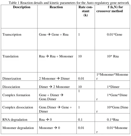
Table 1 Reaction details and kinetic parameters for the Auto-regulatory gene network .. 47
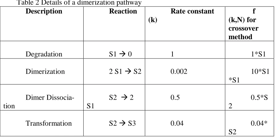
Table 2 Details of a dimerization pathway ... 51
Table 3 Noise levels in critical proteins... 55
Table 4 Details of the HPG axis ... 57
LIST OF FIGURES
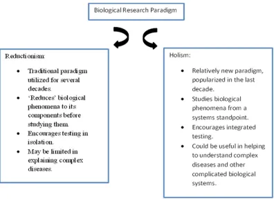
Figure 1 Conceptual differences between the two methodologies employed in biomedical
research ...4
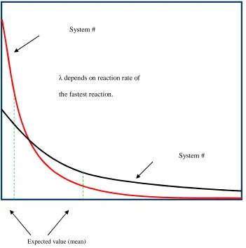
Figure 2 Comparison of the probability distributions for two hypothetical biochemical
systems used for predicting the time-step in the Gillespie algorithm. System # 2 evolves
slower than system # 1. ... 32
Figure 3 Illustration of a Bernoulli trial. A coin toss and a roll of dice are both examples
of a Bernoulli event. ... 36
Figure 4 Illustration of the use of Bernoulli trial to modify a deterministic framework. .. 37
Figure 5 Schematic comparison of continuous and exact stochastic solutions to a system
of differential equations. δt1and δt2 are the errors introduced in the time step ‘t’ of the
continuous solution by the crossover method. ... 37
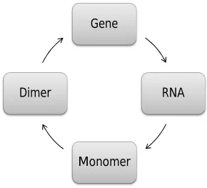
Figure 6 The scheme for an auto-regulatory gene network. The dimer negatively
regulates the gene. ... 46
Figure 7 Results of a single run (left panel) and median of 9 runs (right panel) of
crossover method (red) compared with the results from SSA (blue) and deterministic
(black) method... 48
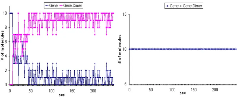
Figure 8 The sum of ‘Gene’ and ‘Gene.Dimer’ stays constant throughout the simulation.
... 49
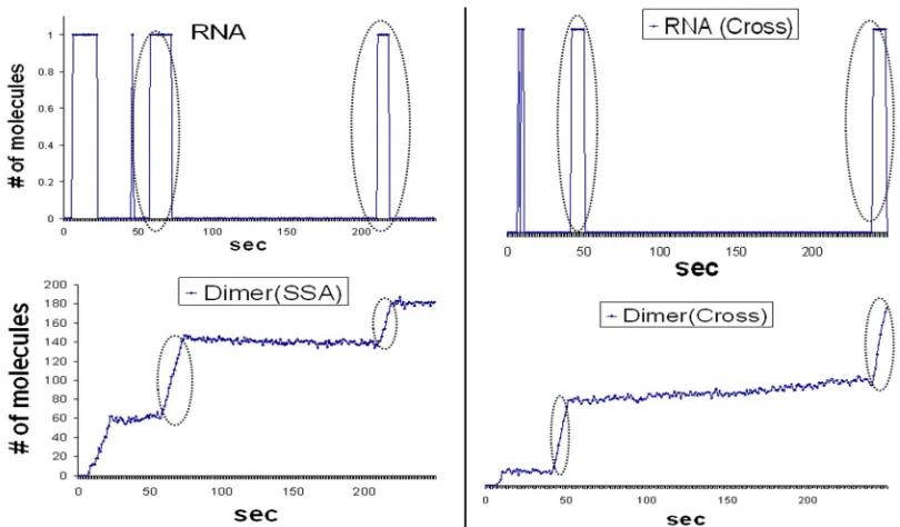
Figure 9 Dimer (bottom) responds to the random fluctuations in RNA (top). These
stochastic effects (dotted ovals) that are normally observed in SSA (left panel) are also
Figure 10 Crossover method displays stochastic effects as the S1 changes into a low
concentration (bottom) from a high concentration (top). ... 52
Figure 11 Stochastic effects are observed when S2 transitions into a lower concentration
(bottom)... 53
Figure 12 The interaction scheme for Blimp-1, Bcl-6 and Pax-5. Arrows indicate negative
regulation. ... 54
Figure 13 Evolution of three proteins critical for terminal B cell differentiation into
plasma cells. ...
... 56
Figure 14 Schematic representation of the HPG axis in vertebrates and its regulation.
Dashed lines indicate negative feedback. ... 57
Figure 15 The simulation output of gonadal hormones of the HPG axis for parameter set
1. Testosterone (left), GnRH and LH (right). Trajectories from A) Deterministic solution
(blue), B) SSA (green) and C) the crossover method (red). ... 63
Figure 16 The simulation output of gonadal hormones of the HPG axis for parameter set
2. Testosterone (left), GnRH and LH (right). Trajectories from A) Deterministic solution
(blue), B) SSA (green) and C) the crossover method (red). ... 63
Figure 17 The simulation output of gonadal hormones of the HPG axis for parameter set
3. Testosterone (left), GnRH and LH (right). Trajectories from A) Deterministic solution
(blue), B) SSA (green) and C) the crossover method (red). ... 64
Figure 18 Comparison of the execution times of the crossover method and the SSA for
1 INTRODUCTION
1.1 Why Study the new paradigm of systems biology?
Complex diseases such as heart disease, cancer and diabetes account for more than half
of human mortality in the United States. Other diseases such as AIDS, asthma, Parkinson’s
dis-ease, Alzheimer’s disease and cerebrovascular ailments such as stroke not only augment the
tality but also severely deteriorate the quality of human life experience. Although the global
mor-tality count associated with HIV-1 infections has abated, failure to produce a vaccine still
per-mits millions of new infections worldwide. In spite of being widely studied and well
character-ized, infectious diseases such as influenza and tuberculosis continue to provide a threat to human
life across the globe. There is no lack of financial support afforded for research in these areas and
has been, in fact, very generous. Each year, for the past four years, the National Institutes of
Health (NIH) in the United States has provided over 10 billion dollars for research projects
in-volving complex diseases like heart disease, cancer and diabetes (http://report.nih.gov). In spite
of the exorbitant financial investment and ever-increasing global scientific research efforts to
combat the challenges posed by these multifaceted ailments, the quest to find a cure or vaccine is
not yet complete (Phair R. D., 2012). It is well known that these complex diseases are not a
re-sult of a single element but a combination of genetic, environmental and lifestyle factors. Other
diseases that are not officially categorized as complex, for example Tuberculosis, are also more
often than not a combination of a variety of physiological factors (Kitano 2007).
1.1.1 Limitations of reductionism
For the past several decades, however, the traditional research paradigm that has been
method of breaking down a biological phenomenon into its constituent components in an attempt
to isolate and characterize the component responsible for the physiologically observed
pheno-type. The conceptual rationale for reductionism is that any physical phenomena can be explained
by a deterministic evaluation of its constituents. An example of this approach is trying to explain
the consciousness of human mind by ‘reducing’ the phenomenon to a set of chemical reactions
occurring in the brain and studying them in isolation (Bickle et al., 2003). This “reductionist”
approach of explaining high-level observations from activity of lower level components has
served the research establishment very well over several decades and has led to a very accurate
functional and structural annotation of the components under consideration. A major drawback
of this approach, however, is that it provides limited insights into the functional properties of the
system itself which can be important for a variety of reasons.
The study of systems biology relates to studying entire biological systems consisting of
many interacting networks that ultimately define the holistic character of any organism including
humans. Conversely, any biological entity can be viewed as nothing but an enormous complex
network of interacting sub-networks (Kitano 2000, 2002). The basic differences between
reduc-tionism and holism are explained in figure 1. It is now widely accepted that an important facet of
any biological system is the property of emergence (Kitano 2002, Van Regenmortel 2004). An
‘emergent’ property is the one that ‘emerges’ as a result of the system components coming
to-gether under specific circumstances and cannot be arrived at by simply adding the components.
For example, the three dimensional conformation of a protein molecule cannot be predicted by
simply lining up the amino acid sequence. The unique folding pattern adopted by the protein can
thus said to be an emergent property of the system. Similarly, biological systems characterizing
im-possible to be studied by the reductionist approach. Hence, a complex disease like cancer cannot
be studied in isolation of the environmental factors without sacrificing emergent properties.
An-other systems property of robustness is very important in the context of drug discovery and
vac-cine development (Kitano 2002). A biological system is composed of biochemical pathways,
gene regulatory networks, signaling pathways, protein interaction networks,
protein-nucleic acid interaction networks and a number of environmental factors engaged in a highly
structured yet complex interaction. Robustness is the ability of this system to adapt to any
per-ceived perturbations in its components. The effect of any one of these components on the entire
network is difficult to analyze with the current molecular biology methods. With most of the
re-ductionist techniques geared towards understanding the function of individual components, it is
almost impossible to predict what effect a local disturbance introduced into the system by a
dis-ease or a drug might have on a distant pathway which may not be part of the current system but
is nevertheless important in terms of function. System robustness is generally achieved via
re-dundancy of components where several parts of the system essentially serve the same purpose
and affecting one of them generally provides no appreciable difference in the overall phenotype.
In reductionism such a component would be simply ignored given the lack of its effect on the
phenotype and in process lose a potential drug target. Redundancy allows the system to be
modu-lar so that a failure in one part of a system does not mitigate to other areas and makes the system
‘robust’ to external insults. Hence from a drug discovery point of view, because diseases are a
result of variation in the biological homeostasis, knowledge of the inherent robustness of the
sys-tem becomes very critical. Global effects of local perturbations in a ‘diseased’ biochemical
net-work are difficult to predict by reductionist techniques that are designed to ignore the property of
It is for these reasons that some researchers argue that reductionism might have hit its
ceiling with regards to biological research (Mazzocchi F., 2008, Van Regenmortel 2004).
Anoth-er criticism of reductionism is that it also requires studying the component of intAnoth-erest extAnoth-ernal to
its natural environment and then attempts to extrapolate the results to the host environment. Such
extrapolation rarely works as evidenced by the failure of knockout mice experiments to be able
to translate to human systems. It is clear from the preceding discussion that employing the
sys-tems level paradigm for investigating biological processes holds significant potential in solving a
variety of complex problems in the areas of rational drug design, vaccine development, cancer
[image:17.612.109.505.344.632.2]therapy, metabolic engineering and personalized medicine.
1.1.2 Advent of high-throughput technologies
One key development that facilitated, and is arguably indispensable for, the shift from
re-ductionism to holism is the advent of high-throughput technologies for biological
experimenta-tion (Resendis-Antonio O., 2011, Nurse P., 2011). A number of technologies such as mass
spec-trometry, DNA / RNA expression microarrays and next-generation sequencing platforms are
now available to the molecular biologists. The literature offers a very detailed review of all the
available technologies (Simpson J. C.., 2006, Segata N., 2008, Chen B. S., 2008). Mass
spec-trometry is widely applied in the field of proteomics where it is utilized primarily for identifying,
quantifying and analyzing novel network components. In this technique, proteins are digested
with proteases and then subjected to liquid phase chromatography and gas phase fractionation.
The spectra thus obtained are used to determine the sequence of the protein. Mass spectrometry
can identify thousands of proteins in a given sample making it an ideal fit for systems biology
(Sabido E., 2011). DNA / RNA microarray technology is primarily used for detecting the up or
down-regulation of RNA transcripts expressed in a biological system. As this technique can also
detect thousands of transcripts at once, it fits nicely into the realm of systems biology. The RNA
fragments to be detected are attached to probes and then hybridized with fluorescence. Laser is
then used to detect the fluorescent intensity and determine the regulation status of RNA
tran-scripts. The data generated by the experiment is then analyzed statistically to draw an inference
and generate hypotheses that can be further tested. Microarray technology was one of the earliest
technologies that helped expedite the molecular biologist’s migration from reductionism to
sys-tems level interrogation. Other high-throughput technologies available target slightly different
areas of biology. For instance, next generation sequencing technologies have revolutionized the
in a matter of afew hours to days as opposed to several months required in the early part of the
last decade. Although the recent high throughput experiments have been successful in providing
a deluge of data to enable a systems view of a biological phenomenon, lack of adequate
technol-ogy for generating meaningful hypotheses without novel experimentation still remains one of the
major hindrances against successful treatment of fatal human diseases.
1.2 Application of systems biology: A literature review
One of the more obvious applications of holistic systems-level biology can be observed
in the process of drug discovery. The exorbitant amount of capital spent on introducing new
drugs in the market and the relatively high number of failed targets in clinical development
war-rants a review of current drug discovery process. Identification of drug targets and developing
drugs against most diseases requires a methodical approach to help decipher the interactions
among the participating biological factors, and ascertain how these factors contribute towards the
etiology of the disease. The advancement of high-throughput technologies in molecular biology
has allowed researchers to genotype and profile thousands of DNA markers and other molecular
phenotypes simultaneously in large number of individuals, thereby permitting the reconstruction
of those biological networks that are known to be associated with a particular disease. These
re-constructed networks are more integrative and predictive thus providing a more insightful
con-text for single genes that have been identified by traditional molecular biology techniques (Zhu
et. al., 2008, Schadt et. al. 2009). Another advantage of systems biology based drug discovery is
that in diseases such as AIDS where drug resistance is a major hindrance towards developing
new drugs, systems biology may be able to provide alternate targets based on the knowledge of
underlying interacting metabolic pathways (Andersen-Nissen E. et. al., 2012). The use of
analyze and integrate large datasets are studied in order to discover novel vaccines for HIV
in-fections (Buonaquro L., et. al., 2011, Haddad E. K., et. al., 2012). In a different approach to
studying HIV pathogenesis, researchers have started focusing on the so called elite controllers of
HIV. The elite controllers are individuals who have defied the presence of the virus in their
sys-tems and show no signs of transforming into full blown AIDS without the help of anti-retroviral
therapy. On a physiological level, holistic approaches are currently being used to study the
dif-ferential regulation of signaling pathways involved in T-cell depletion in these elite controllers of
HIV (Fonseca S.G. et. al., 2011). Systems biology has also been applied to shed more light on
how the sub-networks of an infected host act in concert to limit the damage to its immune system
especially in elite controllers of HIV and natural carriers of SIV (Hoof I. et. al., 2011). A similar
approach has also been reported for understanding the response by exposed uninfected women
(Burgener A. et. al., 2010). Vaccine development using systems biology principles, however, is
not restricted to one single disease and at least one study argues that using systems biology,
in-stead of the narrowly focused ‘isolate, inactivate, inject’ strategy, is a more efficient option for
vaccine development (Oberg A. L. et. al., 2011). Another study reports the application of
sys-tems biology principles in studying the integrated actions of innate and adapted immune
re-sponse as an essential part of vaccine development (Buonaquro L. and Pulendarn B., 2011).
In the area of neuroscience, systems biology has contributed in gaining insights into
mechanisms of synaptic plasticity (Kotaleski J. H. et. al., 2010) as well as addiction (Tretter F et.
al., 2008). Complex neurological diseases such as neurofibromatosis type 1 (NF1) are also being
explored from an integrative systems biology standpoint (Lee M. J. et. al., 2011). An integration
of genome wide association studies with the gene expression data for Parkinson’s disease
approach is adopted in the identifying new biomarkers and drug targets for the treatment of
neo-cortical epilepsy (Loeb J. A., 2010). Geshwind offers an excellent review on how the overall
concept of systems biology can be applied to various areas of neuroscience (Konopka G., 2011).
Understanding the etiology associated with complex medical conditions such as
congeni-tal heart diseases is greatly aided by systems biology (Sperling S. R., 2011) as is an elaborate
un-derstanding of the pathophysiology of heart disease (Dewey et. al., 2011). Recently systems
bi-ology has been instrumental in gaining systemic insight into cardiomyogenesis (Young D. A. et.
al., 2011). Other complex diseases such as cancer also lend themselves as ideal targets for
sys-tems biology based research. Biological cellular networks are routinely deregulated in tumor
me-tastasis. However, the resulting dynamics are not always comprehensible from an experimental
output. Systems based mathematical models are hence important to help make sense of the
com-plex behavior resulting from such a deregulation (Cloutier M. et. al., 2011). An example of this
type of investigation can be cited from a recent study regarding the hyperactivation of PI3k/AKT
pathway, where systems biological approaches were used to predict useful drug targets (Mosca
E. et. al., 2011). Another study focusing on the dynamics of JAK-STAT pathway as related to
cancer focuses on the application of systems biology in modeling cancer-relevant signal
trans-duction networks (Vera J. et. al., 2011). Similarly, work on the role of epidermal growth factor
receptors on cell migration in non-small cell lung cancer is also an extensive demonstration of
the use of systems biology principles (Bianconi F et. al., 2011). From a clinical standpoint,
holis-tic approaches are routinely utilized for identification of novel genes that could contribute to
re-duced efficacy of cancer treatments (Allen W. L. et. al., 2011).
It is clear from the above discussion that, systems biology has indeed been very useful in
par-adigm has been equally well employed. Two of the most impacted areas of molecular biology at
this level are the genetic regulatory system and the signal transduction system. On the genetic
regulation level, systems biology has been used to better understand the role of microRNA in
catalyzing the gene regulation process (Watanabe Y., 2011). As a specific example, in patients
with pancreatic cancer certain miRNAs involved in metastasis were found to be deregulated and
the epigenetic connection for the regulation of these miRNAs was investigated by using holistic
systems biology (Azmi A. S. et. al., 2011). In yeast, the GAL regulon encodes for genes that
al-low the processing of galactose as an energy source. Recently, a systems level interrogation of
this genetic network uncovered certain network properties of substrate regulation and
auto-sensing that are important for the adaption of yeast to its environment (Pannala V. R. et. al.,
2010). Experimental and computational systems biology has also been applied in the area of
gene therapy (Mac Gabhann F. et. al., 2010). High throughput approaches are routinely used in
identifying new members of the signal transduction family of G-protein-coupled receptors
(GPCR) that are intimately involved in signal transduction in the regulation of normal
mammali-an physiological function (Wu J et. al., 2012). In plmammali-ants, the dynamics of abscisic acid (ABA)
signaling pathway are better interrogated by using transcriptome analysis and
‘phosphoprote-omics’ approach (Umezawa T., 2011). Systems biology has also helped better understand the
apoptotic signaling network in eukaryotes (Lavrik I.N., 2010).
1.3 Why is computational systems biology important?
Experimental systems biologyfacilitated via high-throughput experiments are just one
part of the holistic process. The other part is to use a computational modeling methodology to
come up with experimentally testable hypothesis. As pointed out by Kitano in his review on the
other and engage in an iterative process where the quantitative predictions are constantly tested
in wet laboratories and the results are fed back into the computational model to generate refined
hypothesis. Although it is difficult to pinpoint the exact time when simulation of biological
sys-tems originated, it has its roots in the work done on quantitative modeling of kinetics in the
peri-od from 1900-1970. In 1952, Nobel Prize winners Alan Lloyd Hperi-odgkin and Andrew Fielding
Huxley successfully constructed a mathematical model describing the action along the axon of a
neuronal cell (Hodgkin et. al., 1952), which was probably the first notable application of
theoret-ical biology. However, lack of good quality data hindered this area of study from achieving its
full potential, validating the claim that a theoretical model is only as good as the data it works
with. This all changed when high-throughput experiments developed in the 1990s brought a
del-uge of genomic and proteomic data that could be used for quantitative modeling. When this
de-velopment was coupled with a revolution in the computation technology available to scientists,
numerical simulation once again topped the list in scientific discussions. An important
conse-quence of this inclusion of computation technology in life science research was the idea of a
sys-tems level integration of biological components to quantitatively understand the exact behavior
of a biological system. Opposing the traditional view, systems biology tends to analyze any
bio-logical process as a network of interacting systems. There is now increasing consensus among
the scientific community that this systems level perspective is poised to answer a wide range of
biological questions that have immediate consequences in areas of rational drug design, cancer
therapy and personalized medicine. Several methodologies including kinetic modeling,
bio-simulations, predictive metabolism, data mining, and disease modeling are a critical part of
sys-tems biology. Computational syssys-tems biology can hence be defined as a part of syssys-tems biology
using mathematical techniques to provide the ability to make predictions about future
experi-mental hypotheses (Rodriguez et al. 2010). A typical project starts with a reconstructed network
map of all the components of the network which is then translated into a mathematical model
(Sible et. al. 2007). Although the term ‘mathematical model’ can have various implications, in
computational systems biology a mathematical model usually refers to a system of ordinary
dif-ferential equations (ODEs) that has been formulated using the kinetic data available for every
non-constant component of that system. This system of ODE is then solved using appropriate
initial conditions to realize a time course evolution of each component. Once the simulation
re-sults are consistent with previously known experimental observations, this model can be used to
generate predictions for future experiments. The various kinetic parameters that are a part of the
ODE system can be tweaked and twiddled to represent a local perturbation in the network and
the global effects due to the artificial disturbance can be observed from the simulation results.
Thus the ability to simulate a mathematical model that can provide experimentally testable
hy-potheses is central to the systems level study of a biological process. For example, a detailed
mathematical model for TNFα – NFκB signaling was recently developed in conjunction with a
protein-protein interaction map to quantitatively describe the signaling mechanism (Visvanathan
M., 2010). Such a model can now be tweaked around and ‘played with’ to mimic specific
sce-narios as regards to disease or drug intervention and the response in turn could lead to
develop-ment of new hypotheses. Similarly, in the drug discovery process, computational systems
biolo-gy based network analysis enables the action of drug targets to be considered in the context of
the whole genome thus making them an important tool in comprehending the complex
relation-ship between a drug and the target genes (Berger et.al. 2009, Materi W. et. al., 2007). In general,
mathematical / computational modeling is an integral part of such an effort (Ewing G. W., et. al.,
2011, Meyer-Hermann M., et. al., 2009, Groh A., et. al., 2008, Palme K., 2006).
2 MATHEMATICAL MODELING AND SIMULATION
As observed in the previous chapter, systems level investigation of biological processes
holds significant potential in solving a variety of complex problems in the areas of rational drug
design, cancer therapy, metabolic engineering and personalized medicine. The computational
aspect of such an investigation routinely utilizes mathematical modeling techniques to test the
dynamics of a biochemical system and generate experimentally testable hypotheses from them.
The intention to mathematically model a physical system is to create a quantitative
rep-resentation of the role of participating species (reactants) and their interdependent behavior
(re-actions). The first stage of modeling is to create a stoichiometric model by extracting pertinent
information regarding the proportions of reactants in the system. This information is easily
ob-tained from network diagrams and technical literature. Next, a mathematically rigorous
descrip-tion of the system based on classical theory of mass acdescrip-tion kinetics and reacdescrip-tion stoichiometry is
obtained. This mathematical description can vary depending on the framework used for
subse-quent simulation of the model. In the field of biochemical reactions, two simulation frameworks,
deterministic and stochastic, are more popular than others. The work by Crampin E.J. (2004)
provides an excellent overview of the modeling process.
2.1 Deterministic simulation framework
In the widely popular deterministic framework, the goal is to try to represent the behavior
of a homogeneous physical system by a system of ordinary differential equations (ODE) derived
terms of concentration (usually moles/liter) which allows the overall dynamics of the system to
evolve continuously in time. Developed several decades ago, the law of mass action states that
the velocity of an elementary chemical reaction (i.e. a reaction without any intermediates) is
di-rectly proportional to the product of the concentration of the reactants participating in the
reac-tion. The constant of proportionality, called rate constant, is most often a function of the reaction
environment. It logically follows that, the net change in concentration of a reactant of a
biochem-ical system will be the sum of the changes in concentration for every elementary reaction the
re-actant is a part of. Mathematically, for ‘m’ reversible elementary reactions and ‘n’ rere-actants, the
statement can be represented as,
, ↔ , = 1,2 … … … … . … … … . . (1)
where, ‘u’ and ‘v’ in equation (1) are stoichiometric coefficients of reactants and
prod-ucts (S) respectively. In terms of a differential equation, the net rate of change in reactant ‘S’ can
then be written as:
= , = 1 … … . … … … . … … … . (2)
where, ‘R’ is the rate of reaction ‘j’. Applying the law of mass action, we get
, = , − ,
,
− , = 1 … , = 1 … … . … … … . . (3)
cj and c-j are the reaction constants for the forward and reverse reactions respectively. For
example, in the following hypothetical elementary reaction:
+ → +
=− [ ][ ] =− [ ] … . … … … . … … … … (4)
In equation (4), [A] is the concentration of reactant A while ‘c’ is the reaction rate
con-stant. The negative sign indicates that ‘A’ is being consumed as the reaction proceeds. Similar
equations can be written for ‘B’ and ‘C’ as well. Assuming it to be the only reaction in the
sys-tem, the three differential equations (each for A, B and C) taken together would form a system of
ODE for the entire biochemical network and when integrated as a function of time would yield
time course trajectories for all three species reflecting the dynamics of the biochemical network.
The literature offers a more detailed description of kinetic modeling in biological systems
(Gri-ma R., 2011, and Crampin E. J. et. al., 2004). Unfortunately, biochemical reactions cannot
al-ways be characterized by simple elementary kinetics and complex kinetics such as the
Michelis-Menten scheme is often used to describe the reactions more accurately.
The most common situation where the reactions have to be represented by complex
kinet-ics is when a biochemical reaction is catalyzed by an enzyme. The resulting kinetkinet-ics from such
an encounter are inherently non-linear and hence difficult to analyze quantitatively. The most
common enzyme catalyzed reaction scheme is as described in Segel (1975):
+ ⇒ +
‘S’ in the above scheme is the substrate, ‘E’ is the enzyme catalyzing the reaction, ‘ES’ is
the enzyme-substrate complex and ‘P’ is the product. c1f’, c1r are the reaction rate constants for
the forward and reverse reactions of the first half of the reaction while c2 is the rate constant for
the final half of the interaction. The rate of reaction can only be derived using a set of
assump-tions collectively known as the quasi-steady state assumption (QSSA). In the above scheme, it
can be reasonably assumed that the overall reaction is limited by the rate of product formation
= ∙[ ] = … . … … … . . . … … … . (5)
The rate of change of [ES] can be written as,
[ ]
= ∙[ ][ ]− ∙[ ]− ∙[ ] … … … . … … … . . (6)
The first of the QSSA states that, the concentration of the enzyme-substrate complex does
not change over time and hence the first derivative, d[ES]/dt, will be equal to zero. Applying this
assumption to equation (6), we get,
[ ]
= ∙[ ][ ]− ∙[ ]− ∙[ ] = 0 … . … … … . … … … . (7)
Solving for [ES] gives,
[ ] = ∙[ ][ ]
+ … . … … … . . (8)
For simplicity, equation (7) can be rewritten as,
[ ] = [ ][ ] … . … … … . … … … … . . (9)
where, KM is known as the Michelis-Menten constant and is equal to the ratio ((c2
+c1r)/c1f)
Substituting equation (8) into equation (5) gives,
= ∙[ ][ ] … … … . . . (10)
Equation (10) is an acceptable and theoretically correct form of reaction rate expression
except for the fact that the transient concentration of enzyme, [E], cannot be readily measured in
a laboratory. Hence for practical reasons, it is more desirable to use the [E] as a function of total
any given time during a reaction, the total enzyme concentration is equal to the sum of the
transi-ent conctransi-entration and the enzyme associated with the enzyme-substrate complex. Therefore,
= [ ] + [ ] … … … . … … … . (11)
Substituting [E] in terms of [ES], as obtained from (11), in equation (9) gives,
[ ] = {[ ]−[ ]} ∙[ ] … . … … … . … … … . (12)
Solving equation (12) for [ES] gives,
[ ] = [ ]∙[ ]
[ ] + … . … … … . . . (13)
Hence, the rate of reaction becomes,
= [ ]∙[ ]
[ ] + … . … … … . … … … . … . . . (14)
The third and final QSSA states that, the concentration of enzyme, [E] is far less than the
concentration of substrate, or [S] >>> [E], thereby making the maximum reaction rate limited by
the total concentration of enzyme ([Etotal]). So the maximum reaction rate (Vmax) equals the
prod-uct of c2 and [Etotal]. With these adjustments, the rate equation finally takes form as,
= [ ]∙[ ]
[ ] + … . … … … . … … … . . . (15)
Equation (15) is known as the Michelis-Menten equation and quantitatively relates the
in-itial rate of reaction with the substrate concentration for enzyme catalyzed biochemical reactions.
This is the simplest reaction scheme for enzyme catalyzed reactions. Other enzyme mediated
re-actions include competitive, uncompetitive and non-competitive enzyme inhibition as well as
multi-substrate reactions. Needless to say, the rate expressions for those schemes are much more
complicated than equation (15) but are nevertheless based on Michelis-Menten kinetics. Finally,
class of kinetics called sigmoidal kinetics is used to describe them. An expression called the Hill
equation is used to represent the dynamics of such enzymes.
=
+ = + … … … . . (16)
In (16), θ is the fraction of binding sites occupied on the enzyme. ‘S’ is the substrate and
kd is the dissociation constant for the enzyme.
Enzymes obeying the Hill equation are generally allosteric in nature and promote
co-operative substrate / ligand binding. A parameter known as the Hill co-efficient (n) determines
the level of co-operation in binding. It can be clearly seen from the situations above that a
sys-tem of ODE derived from such kinetics would rarely exhibit a linear relationship and as such its
analytical solution may be extremely difficult to attain if not impossible. In such situations,
nu-merical methods have to be employed to approximate a solution of the ODE system. Two main
classes of numerical methods are described below:
2.1.1 Explicit numerical methods
The most intuitive and straightforward methods to solve an ODE are the explicit methods
belonging to a family of methods known as the Runge-Kutta methods. Euler’s method (a.k.a 1st
order Runge-Kutta method) is the simplest explicit numerical solution available to solve an
ODE. The mathematical problem can be stated as an initial value problem: Given an ODE of the
form,
= ( ), ( ) = … … … . … … … … . . (17)
it is required to find an approximate value of the function ‘y’ at time t1 so as to ‘simulate’
Δ
Δ = ( ) =
−
− … … … . (18)
= +ℎ ∙ ( ) … … … . … … … . . . (19)
In general, for i = 1, 2 … n
= +ℎ ∙ ( ) ………..………...… (20)
Equation (20) is the working equation for Euler’s method, where, yi+1 is the value of
function ‘y’ at time ti+1; yi is the value of ‘y’ at time ti (which is known from previous step); ‘h’
is the arbitrarily chosen constant time step equal to ti+1 – ti and f (yi) is the kinetic function
de-rived from the law of mass action. Clearly, equation (7) has to be repeated for ‘n’ steps covering
the entire time period of simulation, T = n x h.
Although Euler’s method is extremely straightforward to implement as an algorithm, it is
also the most impractical of all numerical methods. As can be clearly seen in the above
deriva-tion, the method is most accurate when Δt (or ‘h’) → 0, indicating the necessity of a very small
time step for it to deliver an acceptable approximation to the exact solution. In doing so, because
the period of simulation T is constant, the number of iterations ‘n’ can become very large (as h
→ 0, n → ∞). Although the local truncation error per step is proportional to h2, it can be an
accu-racy nightmare when accrued over large number of iterations. Also, because of the limitation on
the step size, this method is computationally inefficient.
The mid-point method (a.k.a second order Runge-Kutta) is more accurate than the Euler
method. Assuming the problem statement to be the same as before, the equation for the
mid-point method is,
= +ℎ ∙ ( ⁄ ) ……….……….…… (21)
⁄ = + ∙ ( ) ……….… (22)
Equation (22) is used to evaluate function f (yh/2) which in turn enables the use of
equa-tion (21).
The advantage that mid-point method has over the Euler method, in terms of increased
accuracy, comes at a steep price in computational cost. It can be clearly seen that the use of an
additional step per iteration essentially doubles the computational effort while not providing any
significant improvement in accuracy (local error is of order h3 compared to h2 for Euler) or step
size. Unless accuracy is of extreme importance, mid-point method is generally not a good choice
to solve an ODE. Also, even if accuracy is more important, 4th order Runge-Kutta method is
generally twice as accurate as mid-point method.
Runge-Kutta 4th order (RK4) is the most popular explicit method available to simulate a
system of ODE. The working equation for this method can be written as,
= + ( + 2 + 2 + ) ……….… (23)
=ℎ ∙ ( ) ………..… (24)
=ℎ ∙ ( + ) ……….. (25)
=ℎ ∙ ( + ) ………..… (26)
=ℎ ∙ ( + ) ……….… (27)
RK4 has a fourth order global error (O (h4)) and a local truncation error of O (h5). It is
one of the most accurate explicit methods because of the additional ‘k’ factors which essentially
work as correctors for the slope obtained for Euler’s method. RK4 also has a problem with being
computationally intensive but its major criticism stems from its inherent inability to handle ‘stiff’
2.1.2 Implicit numerical methods
It is common in biochemical systems to have some reactions operate at a vastly different
time scale than other simultaneous reactions. This disparity in time scales translates
mathemati-cally into what is described as ‘stiffness’ in the ODE system. Although an exact definition of
stiffness does not exist, it is generally observed when the solution of an ODE does not change
significantly over time but attempting to increase the step-size in order to speed up the
simula-tion causes the solusimula-tion to become unstable. Explicit methods, regardless of their accuracy, are
prone to instability when applied to stiff equations. Implicit methods, on the other hand, are
un-conditionally stable and generally faster.
The backward Euler formula is the most basic implicit method available. Again
consider-ing the problem statement to be the same as in section 2.1.1, the solution equation can be written
as,
= +ℎ ∙ ( ) ………..… (28)
A quick comparison of equation (28) with equation (20) reveals that the earlier
expres-sion is ‘explicit’ in the right hand side where all the terms are known beforehand. In (28)
howev-er, the function ‘f’ has to be evaluated at time ti+1 before proceeding. There are several ways to
handle this challenge but the most common is to replace it with a linear approximation obtained
from Taylor series.
The problem with backward Euler is the same as with the forward Euler method
de-scribed in 2.1.1. Although, backward Euler is stable for stiff problems, its accuracy is limited.
Also, it is much more sensitive to its step-size than other implicit methods. Computationally,
backward Euler is difficult to encode and the marginal improvement in running time is usually
One of the more popular implicit methods is the Adam-Moulton 2nd order method (aka
trapezoidal rule) whose equation is shown below.
= + [ ( ) + ( )] ………...… (29)
This method enjoys several advantages including stability, speed of computation
(be-cause of large step sizes) as well as accuracy (being a second order method). Its accuracy can be
drastically improved by combining an explicit method to ‘predict’ the solution and then ‘correct’
it using the trapezoidal method. Such methods are called predictor-corrector methods and are
ex-tremely useful for differential equations with complex functions.
2.2 Stochastic simulation framework
Deterministic methods have been extremely useful in modeling biochemical systems and
have been used by physical scientists to model cellular behavior for several decades. These
methods, however, are not without limitations (Wilkinson 2006). First, there exist several
bio-chemical systems where the number of interacting reactants is extremely low. A gene regulatory
system is an excellent example of such a system. The concentration of gene molecules in these
systems is so low compared to the overall volume of the cell that using concentration units to
predict the dynamical behavior of the system usually leads to erroneous results. Secondly, some
biological systems are bi-stable and deterministic simulation in general fails to describe the
dy-namics of such systems (Zhang 2010). More importantly, random fluctuations could be
physio-logically important to the dynamics of the overall cell. For example, failure to capture random
fluctuations in genetic regulation might interfere with the prediction of protein translation
dy-namics. Thus random behavior in certain situations can actually be a desired property rather than
2.2.1 Exact stochastic simulation
It is for the need to accurately simulate the biochemical network that stochastic
simula-tion framework was introduced in 1977 by Daniel T. Gillespie. The underlying logic of a
sto-chastic framework is that biochemical reactions occur due to the random collisions between two
or more reacting species. The biochemical species in a stochastic model are represented in terms
of discrete number of molecules instead of concentration and hence the entire system dynamics
can be updated discretely rather than continuously as in a deterministic framework. The reaction
rate parameters in this framework are linearly related to the deterministic kinetic parameters and
serve as hazard functions that identify the probability of a reaction event occurring. If and when
a reaction event occurs, only the reactants corresponding to that particular reaction are updated
while others are left unaltered. Multiple runs of this random procedure yield a mean value for the
state of the system which is then reported. As can be clearly seen, because the system is allowed
to evolve discretely in time, the dynamics of species present in lower numbers of molecules (and
hence lower concentration) can be effectively captured. From a mathematical standpoint, the
sto-chastic framework attempts to adopt a Monte Carlo approach to solve the chemical master
equa-tion (Gillespie D. T., 1992).
( , | , )
= ℎ − − , | , − ℎ ( ) ( , | , )] . (30)
Equation (29) describe the rate of change of probability of system ‘n’ having ‘M’
reac-tions each having parameters ‘c’ and ‘h’. The solution of the equation (30) as obtained by the
stochastic simulation algorithm (SSA) is a probability density function that is a product of two
mutually exclusive and statistically independent random events. The first event is the random
selection of the reaction event that brings about this evolution. The probability functions for the
first event (p1) is an exponential decay function with a decay factor of ‘a’ which is a function of
the parameters ‘c’ and ‘h’. The function for the second event (p2) is a linear function of ‘c’ and
‘h’ and is similar to the one used by the roulette wheel selection process of a genetic algorithm.
= =
As the two events are mutually exclusive and independent, the total probability will be
given by = ∙ .
In this way, the next reaction chosen is always the one having either the most number of
molecules or the one that has the highest propensity based on reaction rate constant or both. On
the other hand, the time step is selected from a continuous function rather than from a discrete
one and that makes this method an ‘exact’ solution to the chemical master equation (Kierzek A.
M., 2002). The algorithm is implemented by the following steps:
Initialize the system with number of reactions, number of initial molecules for every
reac-tion, the type of reaction and the parameters ‘c’ and ‘h’ for each reaction.
Use the parameters to calculate the hazard functions for each reaction.
Pick two random numbers from a uniform distribution.
Use the first random number to generate a time step τ according to the distribution p1
Use the second random number to generate the index for the next reaction according to p2
Update the system according to the reaction stoichiometry.
Update the hazard functions for each reaction.
Repeat the above steps until end of time T
The algorithm has to be run several times to produce trajectories that generate statistically
2.2.2 Approximate stochastic simulation
Computational time can be a drawback for exact stochastic simulation. To tackle this
problem, methods that attempt to combine the best of both deterministic and stochastic
frame-works called hybrid methods are developed (Salis, 2006). Hybrid methods operate on the
prem-ise that any reaction system can be categorized into a subset of ‘fast’ (high concentration) and
‘slow’ (lower concentration) reactions. Both subsets are then simulated simultaneously using the
appropriate simulation method i.e. deterministic for ‘fast’ and stochastic for ‘slow’ reactions. For
a more information on hybrid methods, the work by Bentele M, (2004) provides a much detailed
description. Hybrid methods tend to sacrifice accuracy of simulation results for gain in
computa-tional speed and are hence known as approximate methods. Hybrid methods are not the only
ap-proximate stochastic solutions available. The Tau-leaping algorithm and slow-scale stochastic
simulation algorithm are just a couple of examples of attempts to provide approximate solutions
to stochasticity. For further details the reader is referred to a review by Daniel T. Gillespie
3 DEVELOPMENT OF THE CROSSOVER METHOD
3.1 Why develop a new computational method?
3.1.1 The need for multi-scale modeling
Studying biology at a systems level to investigate emergent network properties
encom-passes a wide spectrum of time scales and physiological detail and as such mandates the use of
multi-scale modeling techniques to construct mathematical models (Meier-Schellersheim M. et.
al., 2009). For example, a seemingly trivial problem of testing the role of a particular enzyme in
an organism would have to include description of genetic regulation and protein-protein
interac-tion at an intracellular level as well as cellular dynamics at a cell populainterac-tion level. The
corre-sponding time scale of reactions can possibly range over a few orders of magnitude and
address-ing this layer of complexity is imperative for effective systems biology.
Multi-scale modeling is typically implemented via either a bottom-up or top-down
meth-od. A bottom-up method starts with the molecular interactions at an intracellular level and makes
its way to the physiological function while top-down method goes the other way. Both methods
have their own benefits. While bottom-up methods seem to be an intuitive approach to build a
model, the biochemistry of a significant number of biological processes is not very well
charac-terized at the cellular level. This forces the model building efforts to stall at the very elementary
stage even if the ultimate physiological phenotype is well understood. Conversely, if the
bio-chemical reaction parameters are known, a bottom-up approach can be used to construct a
com-prehensive model to generate meaningful experimental hypotheses about the physiological
func-tion. A top-down approach, on the other hand, is designed to take an observed higher level
phe-notype and make testable hypotheses about its underlying molecular mechanism. In this
additional details at every relevant layer of biological complexity until the lowest level of detail
is reached. Hypotheses are generated and tested systematically at every level to determine the
optimum path to the following layer. This approach, because it starts from the actual observation,
is reliable in regenerating the phenotype. However, at sub-cellular level, there are several
chan-nels to achieve a desired experimental observation and therefore it is difficult to pin-point the
exact pathway or mechanism responsible for the observed phenomenon. A typical systems
biol-ogy project actually involves a combination of both approaches and the experimental output to
form a hybrid solution. Regardless of the approach used, it is clear that a systems biology
appli-cation has to account for multi-scale complexity as it is the only way to correctly investigate
emergent network properties.
The issue of multi-level complexity becomes even more critical for studying complex
diseases where the mechanism of pathogenesis itself is complex across biological strata (Vicini
P., 2010, Dewey F. E., 2011, Hatzikirou H., 2011). One of the most insightful descriptions of this
issue is observed while studying genesis and metastasis of cancerous cells (Hatzikirou H., et. al.,
2011). As tumor cells originate from a single cell but grow to form a mass of tissue made up of
an ensemble of various cell types, it is imperative to focus on the subcellular scale during
model-ing tumor genesis. At this scale, in addition to carcinogenic biochemical mechanisms, one must
also consider other factors that influence cancerous behavior such as epigenetic regulation. Next,
at the cellular level the interactions between tumor cells and their microenvironment such as
in-tercellular signaling and transport become dominant and have to be accounted for in the model.
Although the spatial scales at these levels do not present any complexity, the time scales do and
the modeling framework has to be able to handle it. Finally, at the tissue scale, the spatial scales
model-ing perspective. Usmodel-ing agent based modelmodel-ing in conjunction with sensitivity analysis to predict
therapeutic targets for cancer is another recent area where multi-scale modeling is applied (Wang
Z., et. al., 2011). The use of multi-scale modeling is also relevant in the area of diabetes research.
For example, the interplay between insulin secretion on a physiological scale and the
inter-cellular events on a higher scale can be understood by simulating models incorporating an
inte-grated scale of detail (Pederson M.G., et. al., 2011). Most of the common heart diseases like
my-ocardial ischemia and arrhythmia can be studied most effectively by looking beyond the simple
genetic association. Building integrative models of mechanism of ventricular arrhythmia in a
healthy as well as diseased heart, models for initiation of arrhythmia and image-based models are
all examples of extensive modeling efforts spanning multiple scales (Trayanova N. A. et. al.,
2009). Such efforts not only help understand the complex mechanisms of heart disease but also
allow testing the efficacy of antiarrhythmic drugs at multiple biological levels (Dux-Santoy L. et.
al., 2011).
The success of systems biology as a paradigm is inherently coupled with the necessity to
develop integrative multi-scale models. Complex diseases, especially, can be studied effectively
only with such a multi-scale approach. While it may seem intuitive to use multi-scale models as
an antithesis to reductionism, it is still a fairly complicated process which is not very well
under-stood. A bigger problem, however, is the lack of an appropriate computational framework to
simulate such a multi-scale model. To encourage researchers into applying systems biology, it is
absolutely essential for the computational biology community to provide them with the tools that
make the effort of building multi-scale models worthwhile. As discussed earlier, building a
quan-titative model and its subsequent simulation are tied together and one is useless without the
complexities in isolation from building a model, the reverse is not true. It is quite likely that the
frequent influx of novel experimental data from high-throughput biological experiments will
have a qualitative impact on the nature of the model being simulated. This would require having
to rebuild the model from scratch as none of the current infrastructure supports partial
modifica-tion of any model. For real time systems biology applicamodifica-tions that have the capability to support
experimental research, it is highly imperative that an appropriate simulation mechanism be
de-veloped that can inherently adapt to the complexities presented by any biological model
multi-scale or not.
3.1.2 Inadequacy of existing simulation frameworks
As discussed in the previous chapter, a plethora of integration methods employing
deter-ministic, stochastic and hybrid techniques exists to simulate mathematical models. However,
their suitability for systems biology, particularly in context to multi-scale modeling, is woefully
inadequate. Here we look at the most popular methods and discuss how their shortcomings can
limit the potential of systems biology.
Limitations of deterministic methods:
The continuous deterministic methods based on ODEs are the most popular methods to
simulate a biological network. All methods in this family are easy to implement and almost all
physical scientists are familiar with them. These methods are generally robust and can handle a
wide range of complex kinetic expressions. In fact, these methods would be a perfect fit for
sys-tems biology if not for one glaring disadvantage: deterministic methods cannot replicate the
ran-dom fluctuations that are ubiquitous in biomolecule copy numbers. Such ranran-domness also
re-ferred to as stochasticity or ‘noise’ is known to play very important role from a biological point
understand-ing how noise at genetic and molecular level leads to variability in gene expression and hence
protein translation (Stewart-Ornstein J. et. al., 2012, Munsky B. et. al. 2012). The effects at
mo-lecular level are often transduced to the metabolic level and therefore it is critical for any
simula-tion method to acknowledge the existence of such noise. Logically it could be deduced that in
multi-scale modeling, where the models often start with a description of lower level
phenome-non, ignoring stochasticity can lead to erroneous results further up the levels. Deterministic
methods are fueled by kinetic rate expressions which do not change with time or with
concentra-tion and hence output a smooth soluconcentra-tion to the system of ODE. The parameters of the kinetic
ex-pressions are often a representation of the average behavior of the system and hence the noise
within the system is impossible to capture by pure continuous functions. The amplitude of these
random fluctuations is generally not very high and at higher concentration of biomolecules the
fluctuations may not make a significant impact thereby making the deterministic solution closely
match the experimentally observed values. At lower concentration, however, the fluctuations can
appear dominant and a deterministic solution may not seem satisfactory. For example, if the
numbers of molecule X are fluctuating between 1000 and 1001, a deterministic value of say
1000.30 seems like a close match. If, however, a molecule Y is varying between 1 and 2, the
de-terministic solution of say 0.95 seems insufficient and maybe even incorrect.
To address this issue, there have been efforts directed towards using stochastic
differen-tial equations (SDE) to model the biochemical reactions. While a detailed discussion about SDEs
is beyond the scope of this work, it is critical to note that SDEs act by simply adding a ‘noise’
term to the regular differential equation and integrating it as an Ito differential term. The results
concentration of less than 3 molecules, the results are generally inaccurate. ODE or SDE based
methods are therefore unsuited for systems biology based applications.
Limitations of stochastic methods:
One of the key developments in the 1970s, with regards to biochemical simulation, was
the development of a Monte Carlo method to accurately solve the chemical master equation.
Popularly called the Gillespie algorithm after its developer Daniel T. Gillespie, this method
pre-dicts which biochemical reaction, from a given biochemical system, is “most likely” to occur and
the time at which it will occur. The fundamental idea behind this method is that if we reduce any
biochemical system to set of elementary molecular reactions it is possible to simulate, within
ac-cepted statistical boundaries, the Brownian motion of molecules. In this way, it ensures that any
random fluctuations that might arise because of the random motion of molecules are effectively
captured.
There are two critical problems, however, regarding its applicability to systems biology.
First, the Gillespie algorithm derives its statistical parameters from the available kinetic data for
the simulated reactions. There is an innate assumption here that these kinetic data are readily
available for every single reaction and that they are accurate. This may not be always true.
Ex-perimental determination of the kinetic parameters is sometimes not possible for certain reactions
while the ones that are possible might have experimental errors in them. The quality of stochastic
simulation trajectory is then dependent on the quality of kinetic data available just as in the
de-terministic method. During the process of modeling if the modeler encounters missing kinetic
data, it is a common practice to lump the missing reactions together and generalize its behavior
with an approximate kinetic expression. The Michelis-Menten kinetic expression is an excellent
Michelis-Menten type of kinetics without significantly sacrificing the accuracy of the solution. It is
rea-sonable to assume that in a complex multi-scale model, Michelis-Menten type of kinetic rate
ex-pressions would be more of a norm than exception and the stochastic method will fall far short of
need.
Second, and more important, issue is with the computational efficiency of the Gillespie
algorithm. This method updates the biochemical system one reaction at a time based on the
pro-pensity of the reaction to occur. This is a major handicap for system with large number of
reac-tions especially when a system scales to a larger size. Another issue is the manner in which the
time step is chosen for the occurring reactions. As shown in figure 2, the algorithm randomly
picks a number from an inverse exponential distribution. The scaling factor (λ) of the distribution
depends upon the kinetics of the reactions and hence the time step cannot be adjusted to make
the simulation run faster. Any attempt to select a bigger time step in essence jeopardizes the
ac-curacy of the method.
Moreover, stochastic simulation methods are not built to handle ‘stiff’ differential
equa-tions. Stiffness in an ODE system occurs when a majority of the reactions evolve very slowly
(low reaction rate) compared to a few fast ones (high reaction rate). As a result, the time
evolu-tion of the system slows down considerably. The reason for this slow down can be explained
Figure 2 Comparison of the probability distributions for two hypothetical biochemical systems used for predicting the time-step in the Gillespie algorithm. System # 2 evolves slower than system # 1.
The two curves in figure 2 represent the probability distribution of the time step for
sys-tems 1 & 2. Assume that the two biochemical syssys-tems are evolving independently of each other.
Also, assume that system # 2 has a reaction that evolves much faster than others making the
scal-ing factor λ higher than system # 1 which consists of reactions with rate constants in the same
order of magnitude. The Gillespie algorithm randomly chooses a value (μ) from this distribution
as its time step for the respective system. The expected value or the value most likely to be
cho-sen for the distribution can be clearly seen to be larger for system # 1 than system # 2. In other
words, system # 1 is morelikely to choose a larger time step and hence evolve faster than system
λ depends on reaction rate of
the fastest reaction.
Expected value (mean)
System #
# 2. In the above example, system # 2 can be described as being “stiff” and is a common
occur-rence in multi-scale models.
Limitations of hybrid methods:
The accuracy afforded by pure stochastic methods such as the Gillespie algorithm is
im-portant for a variety of simulation based applications. To overcome the drawbacks outlined in the
previous section, there has been a rapid development of hybrid methods. These methods can
usu-ally be divided into two categories: The algorithms in the first category classify the biochemical
system into groups of fast and slow reactions and treat them with either deterministic (fast) or
stochastic (slow) methods. The problem with such a classification is that it is not entirely clear as
to what criteria is suitable to justify such a division. Also, in some instances it might be
im-portant to study fluctuations for fast reactions and it would be impossible to do so because they
are solved with a continuous method. Additionally, for stiff systems only a few reactions are fast
which means the total computational efficiency is still controlled by the slow stochastic reactions
thereby nullifying the apparent speed up in performance. The other category consists of methods
that modify the time step calculation in the Gillespie algorithm. These methods generally
re-ferred to as ‘Tau-leaping’ methods approximate a time step for the Gillespie method without
los-ing the statistical significance of the outcome. The limitation of such an approximation is
two-fold: 1) the use of an “approximation” step for a stochastic algorithm is essentially a sacrifice of
accuracy for gain in performance. This loss of accuracy defeats the purpose of using stochastic
simulation in the first place. 2) Even if we accept that the loss of accuracy is minimal, which is
true for some cases, question marks still remain on whether the performance enhancement is