Positioning And Motion Control For Mobile Robot

International Journal of Emerging Technology and Advanced Engineering

498

Positioning And Motion Control For Mobile Robot

S. I. Amer , M. N. Eskander

, Aziza M. Zaki

1,2_{Electronics Research Institute (ERI), Dokki, Cairo, Egypt.}

Abstract - Odometry is the most widely used navigation

method for mobile robot positioning. In this paper motion control and positioning for a mobile robot working in a warehouse is presented. Odometry system configuration and wheel encoder used are detailed. The calculations of the distance travelled compared to the actual measured distance show some difference that are due to internal and external causes. The errors arising during robot working were discussed and suggestions to correct these errors were presented.

Keywords - Mobile robot , Motion Control, Navigation,

Odometry, Positioning.

I. INTRODUCTION

Navigation means the ability to wander in the environment without colliding with obstacles, the ability to determine one's own position, and the ability to reach certain goal locations. The vehicle also can construct an internal representation to its environment on the form of a map. This map can be used in planning paths towards its goals locations.

So, navigation system may imply the following components:

1- Robot positioning system. 2- Path planning.

3- Map building

The positioning system is the most essential component. The role of positioning system is to answer the question " Where am I ?. The answer can be a relative or absolute position to the robot.

Odometry is the most widely used navigation method for mobile robot positioning. It is well known that odometry provides good short-term accuracy, is inexpensive, and allows very high sampling rates. However, the fundamental idea of odometry is the integration of incremental motion information over time, which leads inevitably to the accumulation of errors. Particularly, the accumulation of orientation errors will cause large position errors which increase proportionally with the distance traveled by the robot. Despite these limitations, most researchers agree that odometry is an important part of a robot navigation system and that navigation tasks will be simplified if odometric accuracy can be improved. Odometry is used in almost all mobile robots, for various reasons:-

- Odometry data can be fused with absolute position measurements to provide better and more reliable position estimation [1-3].

- Odometry can be used in between absolute position updates with landmarks. Given a required positioning accuracy, increased accuracy in odometry allows for less frequent absolute position updates. As a result, fewer landmarks are needed for a given travel distance.

- Many mapping and landmark matching algorithms assume that the robot can maintain its position well enough to allow the robot to look for landmarks in a limited area and to match features in that limited area to achieve short processing time and to improve matching correctness.

- In some cases, odometry is the only navigation information available; for example: when no external reference is available, when circumstances preclude the placing or selection of landmarks in the environment, or when another sensor subsystem fails to provide usable data.

In this paper, the odometry navigation system used in a mobile robot system is described and discussed. Section 2, presents the robot positioning system using odometry and the errors that can affect the accuracy of the positioning of the robot, section 3 describes the mobile robot system used and the odometry system, section 4 shows the robot positioning calculations and the encoder used, section 5 presents the motion control subsystem, section 6 gives the conclusions extracted from the work.

II. ROBOT POSITIONING (ODOMETRY)

Odometry is based on simple equations that are easily implemented and that utilize data from inexpensive incremental wheel encoders. However, odometry is also based on the assumption that wheel revolutions can be translated into linear displacement relative to the floor. This assumption is only of limited validity. One extreme example is wheel slippage: if one wheel was to slip on, say, an oil spill, then the associated encoder would register wheel revolutions even though these revolutions would not correspond to a linear displacement of the wheel.

International Journal of Emerging Technology and Advanced Engineering

499

Non-systematic errors are errors that may appear unexpectedly such as when travelling on rough surfaces with significant irregularities, or on slippery floors.

It is noteworthy that many researchers develop algorithms that estimate the position uncertainty of a dead-reckoning robot [3,4]. With this approach each computed robot position is surrounded by a characteristic "error ellipse", which indicates a region of uncertainty for the robot's actual position, figure (1) [3,5]. Typically, these ellipses grow with travel distance, until an absolute position measurement reduces the growing uncertainty and thereby "resets" the size of the error ellipse. These error estimation techniques must rely on error estimation parameters derived from observations of the vehicle's dead-reckoning performance. Clearly, these parameters can take into account only systematic errors, because the magnitude of non-systematic errors is unpredictable [6,7].

Fig. 1 Growing "error ellipses" indicate the growing position uncertainty with odometry.

III. ROBOT SYSTEM DESCRIPTION AND ODOMETRY

SYSTEM

A.Robot System Description

A mobile robot for working in a warehouse is the aim of this work. The robot has the following specifications:

1- Moving forward and backward without rotation. 2- Moving asides (right and left) without rotation. 3- Have a facility to rotate in a complete circle. 4- The control unit and battery charges should be on

the robot itself.

5- The robot battery assembly has total volt 48V (operating voltage of the motors used for driving the wheels).

B. Kinematic and Dynamic Model

The kinematic model takes the velocities of the steering angles and the linear velocity of the robot and transforms it into the generalized coordinate vector. The dynamic model transforms the torques given to it into rotational acceleration of the steering wheels and linear acceleration of the frame.

B.1. Coordinate Frames and Transformations

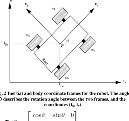
First the robot absolute position in the earth frame has to be described. Figure (2) shows the robot with its center fixed body frame (Ex, Ey) placed inside the inertial frame

(Ix, Iy). The absolute position of the robot with respect to

the inertial frame can be described by the posture vector shown in figure (3).

 = [ x y  ] T (1) The rotation matrix describes the transformation of a point in the inertial frame called Ix,to the body frame Ex.

This is shown in figure (3): Ix to Ex.

Fig. 2 Inertial and body coordinate frames for the robot. The angle

 describes the rotation angle between the two frames, and the coordinates (Ix, Iy)

(2) The transformation from the body frame to the inertial frame is done using the inverse R() -1. Because of R() being an orthogonal matrix, R() -1= R() T

(3)

B.2.Wheels Position

The four wheels of the robot named w1 to w4 are

interconnected two by two such that the angles 1 to 4

seen in Figure ( 3) are related as follows:

1 = 4 and 2 = 3 (4)

B.3. Wheels Rotation Angles

International Journal of Emerging Technology and Advanced Engineering

500

(5)

Fig. 3 The position angle 1 of wheel w1 with respect to the body frame. angle α1 and the argument  describes the position of the

contact point A1

B.4. General Coordinates of the Robot

The three vectors describing the vehicles position, steering angle and wheel rotation angle can be composed to one single vector q, as in eq.(6), which then describes the whole system.

(6)

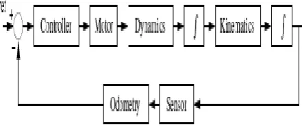
C. General Navigation System

The kinematic modeling of the robot is described in this section after describing the general model of the navigation system. The general model is divided into different components. The overall structure of the system is illustrated on figure (4). The input and output of the different components in the system is shown in table [1].

Fig . 4 Illustration of the system

Table 1

Input and output of the model components.

The system operation is described as follows:

Controller The control law of the system is defined

within the controller. The controller takes the error in position as input and generates the electrical signals for the motors, where a is the armature voltage.

Motors The employed motors takes a voltage as input

and gives torque as output.

Dynamics The dynamic model takes the torque from

the motor model as input, and estimates the accelerations of the system.

Kinematics This part of the model estimates the

velocities according to the inertial earth frame. It takes the linear velocity and the derivative of the steering angles as input.

Odometry This model estimates the position of the

robot with use of the sensor output.

The kinematic model describes the geometrical changes of the robot with the angular velocity . of the wheels and the linear velocity  of the robot as inputs. The output from the model is the change in generalized coordinates q..

International Journal of Emerging Technology and Advanced Engineering

501

The contact between the wheel and the ground is supposed to satisfy the pure rolling without slipping conditions, meaning that the velocity in the contact point between the wheel and the horizontal plane is zero, the wheels does not slip in the ground.

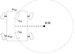
Two kinds of motion for the robot are considered, straight and turning. While the robot is moving in a straight direction, the conditions for pure rolling without slipping are easily satisfied. When the robot is turning, in order to satisfy the constraints of pure rolling without slipping, its motion at each instant can be viewed as an instantaneous rotation around an instantaneous center of rotation ICR whose position to the center of the frame can be varying. It has been assumed that when turning, the robot drives using two fictitious wheels, located in a central fictitious axle, see figure (5). This allows having an ICR around which the robot is rotating and avoids violating the constraints of equal steering angle for each two wheels.

Fig. 5 The robot is assumed to be moving among two imaginary central located wheels when it is turning

Assuming rolling without slipping, the velocity of a point "A" where the wheel touches the ground is given by:

R = VA (7)

From figure (6), we can driven the velocity of the point "A" as:

VA=cos( + i) IA.x + sin ( + i) IA.y (8)

Fig. (6): The velocity components I_A

.xand IA .yare projected into the direction where the wheel is rolling

D. Control Steps

The flowchart of the implemented control algorithm is shown in figure (7). The linear velocity of the robot wheels is fixed to 5 cm/sec, and set as reference speed. The velocity of each motor is then measured at small intervals, checked with the reference velocity. If an error exists, the dc control voltage of the dc brushless motor connected to each wheel is modified and applied to the corresponding motor [8-10].

IV. ROBOT POSITIONING CALCULATIONS

International Journal of Emerging Technology and Advanced Engineering

502

Fig.7 Flowchart for tracking the mobile robot path

A.Rotational Displacement Equipment.

There are different types of rotational displacement and velocity sensors in use today:

1 Brush encoders. 2 Potentiometers. 3 Synchros. 4 Resolvers. 5 Optical encoders. 6 Magnetic encoders. 7 Inductive encoders. 8 Capacitive encoders.

For mobile robot applications incremental and absolute optical encoders are the most popular type, which are discussed in the following sections.

A.1 Optical Encoders

A focused beam of light aimed at a matched photodetector is periodically interrupted by a coded opaque/transparent pattern on a rotating intermediate disk attached to the shaft of interest. The rotating disk may take the form of chrome on glass, etched metal, or

photoplast . Relative to the more complex

alternating-current resolvers, the straight forward encoding scheme and inherently digital output of the optical encoder result in a low cost reliable package with good noise immunity. There are two basic types of optical encoders:

incremental and absolute. The incremental version

measures rotational velocity and can infer relative position, while absolute models directly measure angular position and infer velocity. If non volatile position information is not a consideration, incremental encoders

generally are easier to interface and provide equivalent resolution at a much lower cost than absolute optical encoders.

A.2 Incremental Optical Encoders

The simplest type of incremental encoder is a single-channel tachometer encoder, basically an instrumented mechanical light chopper that produces a certain number of sine- or square-wave pulses for each shaft revolution. Adding pulses increases the resolution (and subsequently the cost) of the unit. These relatively inexpensive devices are well suited as velocity feedback sensors in medium- to high-speed control systems, but run into noise and stability problems at extremely slow velocities due to quantization errors . The tradeoff here is resolution versus update rate: improved transient response requires a faster update rate, which for a given line count reduces the number of possible encoder pulses per sampling interval.

Is Yt = 4.0 m

Set VL=VR= Vlin,

calculate Xt = Xt + Vlin **cos (-/2), Yt = Yt + Vlin **sin (-/2)  = (-/2), and N=N + 

Is Xt = 8.0 m

End Start

Set starting pose (x, y, )Time step  Linear velocity Vlin

Enter Robot Dimensions: L, W and D

Apply gradual voltage "U" to wheel drives and measure 

Is Vlin= set value

Calculate Vlin=  D 

Set t = 1 sec and  = 0

Calculate Xt =no of counts* D/ppr or = Vlin**cos

Yt = Xt tan or = Vlin**sin N= t + 

Set t = t + , and  = 0 Calculate Xt=X t-1 + Vlin *t*cos

Yt = Y t-1+ Vlin, and N= t + 

Is Xt = 4.0 m

Calculate  = 2 Vlin / L , turn= (/2)/ ,

Set VL=-VR= Vlin for t = turn

Set Xt = Xturn, Yt =Y turn, and  =  turn, N =N + turn

Set VL=VR= Vlin,

calculate Xt = Xt + Vlin **cos (/2), Yt = Yt + Vlin **sin (/2)  = (/2), and N=N + 

International Journal of Emerging Technology and Advanced Engineering

503

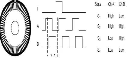
In addition to low-speed instabilities, single-channel tachometer encoders are also incapable of detecting the direction of rotation and thus cannot be used as position sensors. Phase-quadrature incremental encoders

overcome these problems by adding a second channel, displaced from the first, so the resulting pulse trains are 90 degrees out of phase as shown in figure (8). This technique allows the decoding electronics to determine which channel is leading the other and hence ascertain the direction of rotation, with the added benefit of increased resolution.

Fig. 8 The observed phase relationship between Channel A and B pulse

B . Determining Wheel Velocity

Relative position estimation is extremely dependant on the measurement of the robot’s velocity. As mentioned before, for wheeled mobile robot applications, the most inexpensive and most popular are incremental optical encoders. The designed robot is equipped with a phase quadrature incremental optical encoder on each wheel. The spinning wheel produces pulse train square wave signal (i.e., 0 or 1 output). The frequency of the square wave signal corresponds to the rotation speed. The quadrature incremental optical encoders detects direction and angular position (relative to starting position), and has +4 x more resolution than tachometer encoders.

The employed Digital Encoder HEDM-550X provides 1000 pulses alternating between high and low signals. If the robot is moving straight ahead, we could simply count encoder pulses to determine its new location.

Distance traveled per pulse = wheel circumference/ no. of pulses per revolution= 10 /1000=0.0314cm/pulse

While turning is centered around a circle whose diameter equals the distance between wheels (85cm), i.e. whose diameter=267cm

Hence each pulse results in a turn = (0.0314/267)* 360o =0.042o per pulse

The sampling period  is determined approximately by considering the 8-bit counter of the encoder/controller interface HCTL2023 as follows:

Sampling period = (255 counts) / (no of encoder pulses at maximum rotational speed of the brushless motor)

Using the employed motor parameters and ratings the maximum rotational speed max= 12200rpm =

203.3333rps

Hence Sampling period = (255 counts) / 203.3 = 1.2msec

V. MOTION CONTROL SUBSYSTEM

The block diagram showing the layout of the components employed in motion control is presented in figure (9). Two microcontrollers were used. A slave microcontroller is used for controlling the 4-wheels motion. Besides the main components, the optical encoder HEDM-550X, the encoder interface IC HCTL 2032, and the slave microcontroller chip AT90S8535, latches, buffers, crystal oscillators, digital to analog converters are also employed.

The shown layout is briefly explained as follows: Each shaft encoder HEDM-5500 produces two out-of-phase pulse trains which are fed to one of the two quadrature decoder/counter interface IC of type HCTL-2032. The HCTL-2032 accepts the A, B and index connections from the incremental encoder and stores the accumulated count pulses in a dedicated 16-bit time base. If phase A leads phase B, then the direction of the motor is forward. If phase A lags phase B then the direction of the motor is reversed. All peripherals necessary to interface the optical encoder to the microcontroller, and the microcontroller to the wheel drives are determined. These peripherals include decoders, address decoders, latches, buffers, and digital to analogue converters. Latches are used to sense overflow or underflow. Other latches are employed to store the speed commands of the four wheels. Also a latch is employed to decide the direction of wheel rotation.

Calculation of the actual speed and traveled distance is done in the slave microcontroller, in which the reference speed and the time interval are stored.

Any error in the command speed of each wheel, output from the microcontroller, is changed into analog signal fed to the motor driving the corresponding wheel. Buffers are employed wherever needed.

VI. CONCLUSIONS

International Journal of Emerging Technology and Advanced Engineering

504

The errors can be systematic resulting in inaccuracy in the wheels system on non-systematic that are caused from the working environments of the robot such as surface roughness, slippery surface…

During testing the robot system navigation using odometry, errors in the calculation of its positioning was measured. To overcome this difficulty, it was decided

that another navigation aid such as ultrasonic sensors should be used to correct the positioning calculated by odometry at constant time intervals. This correction will be conducted using artificial landmarks or natural landmarks.

Fig.(9) Block Diagram of Motion Control

REFERENCES

[1 ] F.Chenavier and J.Crowley, "Position Estimation for a Mobile Robot using Vision and Odometry," Proc. of IEEE Int. Conf. on Robotics and Automation, ICRA'92, Nice, France, May 12-14, pp.2588-2593.

[2 ] J.M.Evans, "HelpMate: An Autonomous Mobile Robot Courier for Hospitals" Proc. of the Int. Conference on Intelligent Robots and Systems, IROS'94, Munich, Germany, Sept 12-16, pp.1695-1700.

[3 ] Y. Tanoushi, T. Tsubouchi, and S. Arimoto, "Fusion of Dead-reckoning Positions with a Workspace Model for a Mobile Robot by Bayesian Inference", Int. Conf. on Intelligent Robots and Systems, IROS'94, Munich, Germany, Sept 12-16, pp.1347-1354. [4 ] K. Komoriya, E. Oyama, Position Estimation of a Mobile Robot

Using Optical Fiber Gyroscope (OFG)", Int. Conf. on Intelligent Robots and Systems, IROS'94, Munich, Germany, Sept 12-16, pp.143-149.

[5 ] M. Adams et al, "Control and Localisation of a Post Distributing Mobile Robot", Int. Conf. on Intelligent Robots and Systems, IROS'94, Munich, Germany, Sept 12-16, pp.150-156.

[6 ] J.Borenstein and L.Feng, "Measurement and Correction of Systematic Odometry Errors in Mobile Robots", IEEE Journal of Robotics and Automation, May 1995.

[7 ] K.S. Chong and L.Kleeman, "Accurate Odometry and Error Modelling for a Mobile Robot", Int. Conf. on Robotics and Automation, 1997, pp.2783-2788.

[8 ] T D Barfoot, "Odometry for Four-Wheeled Vehicles", Technical Report, University of Toronto, Institute for Aerospace Studies, 16 May, 2003, <[email protected]>

[9 ] E.Olson, " A Primer on Odometry and Motor Control", December 2004.