Predicting Head Pose From Speech
David Greenwood
A thesis presented for the degree of
Doctor of Philosophy
School of Computer Science
University of East Anglia
United Kingdom
April 2018
David Greenwood
2018
Abstract
Speech animation, the process of animating a human-like model to give the impression it is talking, most commonly relies on the work of skilled animators, or performance capture. These approaches are time consuming, expensive, and lack the ability to scale. This thesis develops algorithms for content driven speech animation; models that learn visual actions from data without semantic labelling, to predict realistic speech animation from recorded audio.
We achieve these goals by first forming a multi-modal corpus that represents the style of speech we want to model; speech that is natural, expressive and prosodic. This allows us to train deep recurrent neural networks to predict compelling animation.
We first develop methods to predict the rigid head pose of a speaker. Predicting the head pose of a speaker from speech is not wholly deterministic, so our methods provide a large variety of plausible head pose trajectories from a single utterance. We then apply our methods to learn how to predict the head pose of the listener while in conversation, using
Predicting Head Pose From Speech
David Greenwood
© This copy of the thesis has been supplied on condition that anyone who consults it is understood to recognise that its copyright rests with the author and that use of any information derived there from must be in accordance with current UK Copyright Law. In
addition, any quotation or extract must include full attribution.
I want to thank...
I first want to thank Barry-John Theobald. Quite simply, Barry allowed me to believe I could do this work, and set me off on the path that brought me to where I am now. When Barry’s great talents were recognised elsewhere, Stephen Laycock and Andy Day provided the steady guidance and support I needed, and I warmly thank them both.
I especially want to thank my wife Jayne, and my children Lilly, Tom and Ben. You are the most important people in my world, thank you for giving me the things no one else could, that helped me so much along the way to my goal.
I must thank all the people who I met during the course of this work, and before, who gave insight and advice; you are so many I can’t name you all.
Last, but definitely not least, I want to thank Iain Matthews. Without Iain, so much of this work would not have been possible.
Abstract i Declaration ii Dedication iii Acknowledgements iv Contents iv List of Figures x
List of Tables xiv
1 Introduction 1
1.1 Motivation and Research Objective . . . 2
1.2 Contributions . . . 3
1.3 Publications . . . 3
1.4 Thesis Outline . . . 4
2 Literature Review 5 2.1 Speaker Head Motion . . . 5
2.2 Listener Head Pose . . . 9
2.5 The Uncanny Valley . . . 16 3 Corpus 19 3.1 Actors . . . 19 3.2 Video . . . 19 3.3 Audio . . . 20 3.4 Tracking . . . 23
3.4.1 Active Appearance Models . . . 23
3.4.2 Model Fitting . . . 24
3.5 Camera Calibration . . . 26
3.5.1 Pinhole Camera Model . . . 26
3.5.2 Distortion Parameters . . . 28
3.6 Stereo Triangulation . . . 29
3.7 Data Processing . . . 32
3.7.1 Annotation . . . 32
3.7.2 Shape Model . . . 32
3.7.3 Separation of Deformation and Transformation . . . 33
3.8 Remarks on Data Collection . . . 37
3.8.1 FutureWork . . . 38
4 Feature Extraction 39 4.1 Audio Features . . . 39
4.1.1 Mel Frequency Cepstral Coefficients . . . 40
4.1.2 Vocal Tract Model . . . 43
4.1.3 Energy . . . 44
4.1.4 Pitch . . . 44
4.1.5 Filter Bank Features . . . 45
4.2 Trained Audio Features . . . 47
4.2.3 Network 1 . . . 50
4.2.4 Network 2 . . . 51
4.2.5 Trained Features Results . . . 52
4.2.6 Trained Features Discussion . . . 54
4.3 Forced Alignment . . . 55 4.4 Phonemes . . . 55 4.5 Text Parsing . . . 59 4.6 Word Embedding . . . 60 4.7 Discussion . . . 62 5 Neural Networks 63 5.1 Multi-Layer Perceptron . . . 64
5.2 Recurrent Neural Networks . . . 65
5.3 Long Short Term Memory . . . 68
5.4 Bi-Directional Long Short Term Memory . . . 72
5.5 Generative Models . . . 73
5.5.1 Autoencoders . . . 74
5.5.2 Variational Autoencoders . . . 75
5.5.3 Conditional Variational Autoencoder . . . 76
5.6 Dropout . . . 77
5.7 Data Augmentation . . . 78
5.8 Alternate Models . . . 79
5.8.1 Hidden Markov Models (HMMs) . . . 79
6.1 Related Work . . . 83
6.2 Corpus . . . 84
6.2.1 Data Augmentation . . . 84
6.3 Evaluation and Existing Baselines . . . 87
6.3.1 Canonical Correlation Analysis (CCA) . . . 88
6.3.2 Head Pose Expectation . . . 90
6.3.3 User Preference . . . 92
6.4 Model Topology . . . 93
6.5 Bi-Directional Long Short Term Memory . . . 93
6.5.1 Training . . . 94
6.5.2 Audio Features . . . 95
6.5.3 Phone Features . . . 100
6.6 Conditional Variational Auto Encoder . . . 104
6.6.1 Training . . . 104
6.6.2 CVAE Results . . . 105
6.7 Subjective Testing . . . 112
6.8 Comparison with Prior Work . . . 114
6.9 Discussion . . . 115
7 Listener Head Pose 118 7.1 Motivation . . . 119 7.2 Corpus . . . 119 7.3 BLSTM model . . . 122 7.3.1 Training . . . 123 7.3.2 Results . . . 124 7.4 CVAE Model . . . 127 7.4.1 Training . . . 129 7.4.2 Results . . . 129
8 Facial Expression 135
8.1 Related Work . . . 136
8.2 Dimensionality Reduction . . . 136
8.3 Audio Features to PCA Shape Values . . . 140
8.3.1 Subject A Results . . . 142
8.3.2 Subject B Results . . . 146
8.3.3 Audio to PCA discussion . . . 148
8.4 Phone to PCA Shape Values . . . 149
8.4.1 Phone Model Results . . . 150
8.4.2 Phone Model Discussion . . . 154
8.5 Principal Components to Head Pose . . . 154
8.5.1 Principal Components to Head Pose Results . . . 155
8.6 Joint Learning of Facial Expression and Head Pose . . . 157
8.6.1 Model Description . . . 158
8.6.2 Training . . . 160
8.6.3 Joint Learning Results . . . 160
8.6.4 Subjective User Study . . . 161
8.7 Comparison with other methods . . . 165
8.8 Discussion . . . 168
9 Discussion 169 9.1 Contributions . . . 170
List of Figures
2.1 The Uncanny Valley . . . 16
3.1 The two actors. . . 20
3.2 Cameras are arranged in a radial pattern. . . 21
3.3 Three cameras synchronised to give multi-view stereo. . . 21
3.4 Subject B has three synchronised cameras. . . 22
3.5 Point Distribution Model (PDM) for Speaker A, centre camera. . . 25
3.6 Illustration of an ideal pinhole camera. . . 27
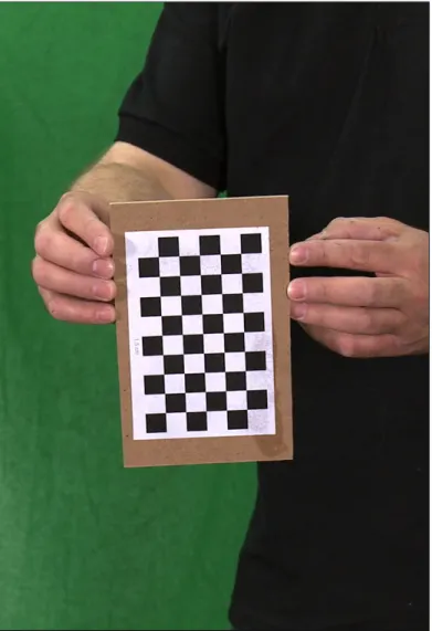
3.7 Cameras were calibrated using a chequerboard pattern. . . 30
3.8 Epipolar geometry. . . 31
3.9 Two stereo pairs allow the triangulation of two sets of 3D points. . . 31
3.10 A neutral pose for each speaker. . . 34
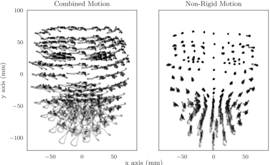
3.11 Separating the rigid and non-rigid motion of Speaker A. . . 35
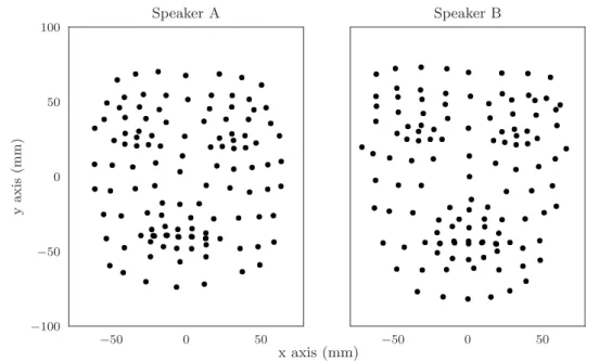
3.12 Here we plot the motion of the landmarks on Speaker B. . . 35
4.1 Feature extraction. . . 39
4.2 Feature alignment. . . 41
4.3 Mel scaled filter bank . . . 42
4.4 Our standardised Audio Feature: Log Filter Bank (LogfBank) . . . 46
4.5 Learning features, Network 1. . . 51
4.6 Learning features, Network 2. . . 52
4.7 Words are force aligned to the waveform. . . 55
4.8 Phones are force aligned to the waveform. . . 58
4.9 A phone is emitted at the sample frequency of the motion. . . 58
4.11 Corpus vocabulary word embedding. . . 61
5.1 Neural Network complexity. . . 63
5.2 The MLP is the basic building block of the ANNs used in this work. . . 65
5.3 A compact diagram for the Multi-Layer Perceptron (MLP). . . 66
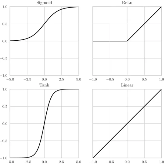
5.4 Activation functions. . . 67
5.5 An RNN has cyclic feedback. . . 68
5.6 Unrolled RNN. . . 69
5.7 Many to many RNN. . . 70
5.8 Asymmetric RNN. . . 70
5.9 Temporal compression RNN. . . 71
5.10 Temporal inflation RNN. . . 71
5.11 LSTM data flow diagram. . . 72
5.12 The deep BLSTM. . . 73
5.13 Autoencoders compress data via a latent space. . . 74
5.14 Variational Autoencoder. . . 75
5.15 Conditional Variational Autoencoder. . . 77
6.1 The axes of head rotation. . . 81
6.2 The head pose trajectory of Subject A. . . 82
6.3 Distribution of Speaker head pose angle. . . 85
6.4 CCA evaluation . . . 89
6.5 Comparing the same transcript repeated by Subject B. . . 91
6.6 User preference of head pose 1 . . . 92
6.11 Head pose results for Subject B from audio features 2. . . 99
6.12 Results for Subject A for phone features 1. . . 101
6.13 Results for Subject A for phone features 2. . . 102
6.14 The topology of the CVAE. . . 105
6.15 Results for Subject A CVAE model, example scene 1. . . 106
6.16 Results for Subject A CVAE model, example scene 2. . . 107
6.17 Results for Subject B CVAE model, example scene 1. . . 108
6.18 Results for Subject B CVAE model, example scene 2. . . 109
6.19 100 random samples of nod trajectory. . . 110
6.20 Extracts from an animation of speaker A. . . 111
6.21 The data collected from a user study. . . 113
6.22 Qualitative counterpart example. . . 115
7.1 Listener head pose . . . 118
7.2 Motivation for learning listener pose from audio. . . 120
7.3 Distribution of Listener head pose angle. . . 121
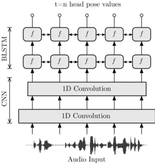
7.4 Modelling listener head pose with a BLSTM. . . 123
7.5 Listener head pose plot Subject A. . . 124
7.6 Listener head pose plot Subject A. . . 125
7.7 Listener head pose plot Subject B. . . 126
7.8 The topology of the listener CVAE. . . 128
7.9 CVAE result for Subject A listening. . . 130
7.10 CVAE result for Subject B listening. . . 131
7.11 100 variations on listening. . . 133
8.1 The 3D deformations over time. . . 135
8.2 Reconstructing the deformation shape for Subject A. . . 138
8.3 Reconstructing the deformation shape for Subject B. . . 139
8.6 Speaker A result for prediction from audio features. . . 142
8.7 Detail result for prediction from audio features for Speaker A. . . 145
8.8 Subject B result for prediction from audio features. . . 146
8.9 Detail result for prediction from audio features for Subject B. . . 147
8.10 Speaker A result for prediction from phones. . . 151
8.11 Detail result for prediction from phone features for Speaker A. . . 152
8.12 Predicting head pose from principal components. . . 156
8.13 The topology of the deep BLSTM model. . . 159
8.14 Prediction of joint learning expression values. . . 162
8.15 Prediction of joint learning head pose values. . . 163
8.16 The data collected from a user study. . . 164
List of Tables
4.1 Speaker A and B correlation coefficients. . . 48
4.2 Correlation with higher dimension features. . . 49
4.3 Spectral features for speaker A and B . . . 50
4.4 Results for each network showing correlation. . . 54
4.5 CMU Phonemes Table. . . 57
4.6 The parse table for our example utterance. . . 59
6.1 Distribution of Subject A head pose angle. . . 86
6.2 Distribution of Subject B head pose angle. . . 86
6.3 Baseline results for head pose prediction. . . 87
6.4 CCA against sinusoid and linear variables. . . 89
6.5 Comparing the same transcript repeated by Subject B. . . 90
6.6 Head pose results for Subject A from audio features. . . 96
6.7 Head pose results for Subject B from audio features. . . 99
6.8 Head pose results for Subject A from phone features. . . 102
6.9 Head pose results for Subject A for CVAE model. . . 108
6.10 Head pose results for Subject B for CVAE model. . . 109
6.11 Speaker head pose user study. . . 113
6.12 Sensitivity index of speaker user study. . . 113
6.13 Comparison of our method with related work. . . 114
7.1 Distribution of Subject A listening head pose angle. . . 120
7.2 Distribution of Subject B listening head pose angle. . . 122
7.3 Listener head pose results for Subject A from audio features. . . 126
7.5 Listener head pose results for Subject A for CVAE model. . . 132
7.6 Listener head pose results for Subject B for CVAE model. . . 132
8.1 Predicting facial variation during speech from audio features. . . 144
8.2 Subject A reconstruction loss during speech from audio features. . . 144
8.3 Speaker B prediction of facial variation during speech from audio features. . 148
8.4 Speaker B reconstruction loss during speech from audio features. . . 148
8.5 Speaker A predicting facial variation during speech from phone features. . . 153
8.6 Speaker A reconstruction loss during speech from phone features. . . 153
8.7 Comparison of Principal Component Analysis (PCA) models. . . 153
8.8 Results for PCA to Head Pose. . . 156
8.9 Quantitative evaluation for joint learning of face and head pose. . . 161
8.10 Joint Modality user study. . . 164
8.11 Sensitivity index of user study. . . 164
8.12 Comparison of quantitative results. . . 166
1
Introduction
Speech animation involves transforming and deforming a human-like model, temporally synchronised to an audible utterance, to give the appearance that the model is speak-ing. The problem is challenging, as human viewers are very sensitive to natural human movement. Practical applications of speech animation, for example computer games and animated films, often rely on motion capture devices or laborious hand animation. Both of these approaches are expensive, time consuming and are unable to scale. Content-driven animation is rich and complex motion derived from easily obtained sparse input, offering appealing properties of lower costs, faster production, and scalability. However to date, there have been few convincing examples.
Human discourse essentially flows in two modes: the explicit mode of audible speech that carries the semantic meaning of some utterance, and a more supportive visual mode where non-verbal gestures complement and enhance the audible mode. Research suggests that speech and gesture may stem from the same internal process and share the same semantic meaning.
There are significant differences between these modes that are pertinent to the work in this thesis. Speech can be processed as a language. A language has grammatical rules and structure and has no ambiguity in meaning. Collecting speech data is relatively easy, and processing is fast and efficient on modern hardware.
Non verbal communication, on the other hand, is far less well understood. There have been many efforts to understand the meaning of gesture. Much of this work seeks a taxonomy, for example Birdwhistell [1952] proposes an equivalent to phonemes, dubbed ‘kinemes’ to describe such action. Ekman and Friesen [1978] develop the Facial Action Coding
tem(FACS), to account for the motion of the face. Although it appears, with the advent of pocket video cameras, as simple to capture visual speech as audio, the issues extend beyond mere hardware. Notwithstanding any discussion regarding the accuracy of the FACS anal-ogy, to extract the coding from video is non trivial. In fact, any such taxonomy requires human experts to create an annotation, a clear limit to scalability.
The central aim of this thesis is to develop models that can learn visual actions from data without semantic labelling, and then, provide compelling speech animation from easily recorded sound.
1.1
Motivation and Research Objective
The pose of the head during speech has interesting properties that present unique modelling challenges. Some activity on the head, most obviously the motion of the lips, the jaw, gen-erally theorofacial area have an obvious direct correspondence with speech. Lip accuracy is important, as mismatches between audio and visual can change what a viewer believes they have heard [McGurk and MacDonald, 1976]. Other activity, perhaps the upper facial areas, and notably, the rigid transformations of the skull appear to be independently controlled, yet have been shown to have correspondence with speech, and even contribute to speech comprehension [Munhall et al., 2004].
Increasingly, we find ourselves in a world with great demands on high quality animation, not only for the most obvious use cases within the motion picture and gaming industry, but also for projecting our presence remotely whether on screen, or indeed, immersive virtual reality environments. We also see increasing requirements for high quality animation for therapeutic use.
Predicting Head Pose From Speech
that is less clearly connected; motion with non deterministic output that must still appear appropriate and plausible.
1.2
Contributions
Our key contributions to the field are three fold. First, we introduce a data-driven method to predict a diverse range of rigid head pose that dispenses with the idea that learning from speech data requires labelling or categorising the motion. We achieve this by de-veloping a corpus that closely represents the emphatic style of speech we find in natural, unrestrained discourse. By recognising that gestures that accompany speech have a many to many relationship, we introduce the Conditional Variational Autoencoder (CVAE) to the task of modelling the rigid pose of the speaker’s head. Not only does our method ac-commodate this difficult task, we gain scalability as our model differentiates the style of multiple speakers.
Secondly, the head pose of the listener in dyadic conversation provides important cues for the speaker. We show that we can directly learn from the voice of the speaker, without resorting to labelling moments of response, or following rule based algorithms, to synthesise these important listener responses.
Finally, the pose of the head is part of a complex bio-mechanical system that may not be best modelled by considering individual components. We develop an algorithm that allows us to predict lip sync, facial expression and rigid head pose, directly from speech. The end result is animation that is visually coherent, accurate, convincing and well received by viewers.
1.3
Publications
The following publications have resulted from the work in Chapters 6, 7 and 8:
• Predicting Head Pose from Speech with a Conditional Variational Autoencoder, Greenwood, D., Laycock, S., and Matthews, I. In Proceedings of InterSpeech 2017, pages 3991–3995.
• Predicting Head Pose in Dyadic Conversation,
Greenwood, D., Laycock, S., and Matthews, I. InInternational Conference on Intel-ligent Virtual Agents, pages 160–169.
• Joint Learning of Facial Expression and Head Pose from Speech,
Greenwood, D., Matthews, I., and Laycock, S. In Proceedings of InterSpeech 2018, pages 2484-2488.
1.4
Thesis Outline
This document is structured into three main parts:
In Chapter 2 we first discuss the history of co-speech activity of the head, and why it represents a difficult modelling task, best approached by learning from data.
Chapter 3 describes in detail the development of a multi-modal corpus that we use to learn appropriate speech animation. We describe our methods of speech feature extraction in Chapter 4 and in Chapter 5 we describe the tools we select and develop for modelling from our data.
Chapter 6 describes how we model the rigid head pose of the speaker learnt from data. We go on to describe the modelling of the listener’s head pose in dyadic conversation in Chapter 7, and finally we describe how we can predict the full facial expressionand rigid head pose of the speaker in Chapter 8.
2
Literature Review
This chapter reviews related work in modelling co-speech gesture and expression, focusing on the motion of the head, the expression of the face and the motion of the lips. We also touch on other co-speech activity involving manual gesture as some of the discussion has relevance for head motion. Finally, we close this section with views on the difficulty of modelling human likeness.
2.1
Speaker Head Motion
Speaker head motion is a rather intriguing aspect of visual speech. Head motion has been shown to contribute to speech comprehension, [Munhall et al., 2004] yet, unlike the articu-lators, it is under independent control. As the speech channel contains the most complete information stream in an utterance, it is a reasonable strategy to seek a mapping from within this stream that might enable plausible predictions of head pose. Indeed, many authors have been motivated by the significant measurable correlation between speech and head motion Deng et al. [2004]; Busso et al. [2005]; Hofer and Shimodaira [2007]; Busso et al. [2007].
When we speak, we encapsulate the semantics of our utterance in the words of our language. We have already stated that rigid head motion is strongly tied to speech, but consider how that occurs. For example, if we are expressing agreement, nodding the head is a common gestural supplement. However, just considering that simple gesture, speaking the same utterance at another time could well have the nodding action at a different phase or frequency. In considering just that simple case, we can appreciate that head pose should be considered as a one to many mapping. And yet there is more to it. When we speak naturally,
we do not issue a monotone dialogue, our voices are highly animated. We use expression, emphasis, intonation orprosody to make speech much more than merely words. With that in mind, we must consider that speech to head motion has a very diverse expectation.
It is interesting to consider the variety of approaches to synthesising the movement of the head during speech. Early approaches depend on hand labelling of audio or text input to form rule based systems, although some of these systems extend their output target to facial expression and manual gesture. Later work is inspired by Automatic Speech Recognition (ASR) techniques, particularly the Hidden Markov Model (HMM). More recent approaches use Artificial Neural Networks (ANNs), but we had to wait for the development of Graphics Processor Unit (GPU) processing for this idea to gain traction.
More than twenty years ago Cassell et al. [1994] presented a system claiming that it:
“. . . automatically generates and animates conversations between multiple human-like agents with appropriate and synchronised speech, intonation, facial expressions, and hand gestures”
Perhaps we would not recognise the animation as being very lifelike today, but the impor-tance of the synchronisation of speech with emotion, gesture, gaze, facial expression and all other aspects of visual prosody was central to its concept. Using a rule based approach, the system tied together audio speech synthesis, facial animation, based on Ekman’s FACS, and a gesture generator using a look-up in a table of predefined gestures.
At the turn of the century, HMMs are the de facto standard in ASR applications [Young et al., 1997; Rabiner, 1989]. Many of the methods for ASR are recognised as applicable for the speaker head pose task by a number of authors. Busso et al. [2005] describe a method using a data-driven approach to synthesise appropriate head motion by sampling
Predicting Head Pose From Speech
They capture the close temporal relation between head motions and acoustic prosodic fea-tures using a bi-gram model trained from multi-modal data, similar to the language models used in speech recognition. The output from HMMs is not continuous, so the head motion must be represented discreetly. For this reason, the Linde-Buzo-Gray Vector Quantization (LBG-VQ) algorithm [Linde et al., 1980] is used to define kdiscrete head poses.
Busso et al. [2005] quote results using Canonical Correlation Analysis (CCA) of r ≈ 0.8, although it is worth noting that the data they collect displays similar levels of prosodic correlation, which is regarded as highly dependent on context and speaker [Yehia et al., 2000]. Their approach involves considerable post processing as the model outputs a square waveform.
Hofer and Shimodaira [2007] maintain the HMM approach but add the refinement of mod-elling head motion from trajectories [Zen et al., 2007]. Of particular note are the correlation analysis results. Hofer and Shimodaira [2007] seek to verify the claims of Busso et al. [2005], but record the correlation within their own corpus as somewhat lower,r ≈0.08. This rep-resents further confirmation of the dependency on context and speaker.
More recently, Ben Youssef et al. [2013] proposed an improved clustering for motion. Whether clustering or quantisation, all of these approaches rely on a suitable labelling of the resulting motion units, either manually or automatically, which is a challenging problem in itself.
Kuratate et al. [1998] presented a paper describing a system that recorded facial motion using opto-electronic tracking to record a speaker’s movements. Kuratate et al. [1998] made a sequence of laser scanned polygonal models of the speaker, capturing vowel visemes and non verbal facial poses during speech. Using PCA they decomposed the polygon data and created a parametric representation that could be controlled with the first five principal components. A linear estimator allowed the mesh to be controlled by the 18 tracked markers. Their model is effectively an Active Appearance Model (AAM).
Following on from this work, [Yehia et al., 2000] established figures showing the correlation between head pose and Fundamental Frequency (F0) speech features:
“ The experimental results show that about 80% of the variance observed for F0 can be determined from head motion.”
It was noted however that the reverse mapping was far less: 25 to 50%, and further, these figures are highly speaker and utterance dependent.
Building on his earlier work, Kuratate et al. [1999] used the correlation between prosodic au-dio features and the motion of facial features to drive the speech animated model, the multi-linear mapping between different modalities, (speech data and Electromyography (EMG) recordings of facial motion) was transformed using a small ANN of ten sigmoid neurons. Recent advances using the GPU [Bergstra et al., 2010; Jia et al., 2014] permit much larger and expressive models.
Li et al. [2013] argues that predicting head motion is better modelled as a regression problem noting that classification relies not only on the definitions of typical head motion patterns, but also the accurate recognition of these patterns. As well, the relationship between speech and head motion is regarded as a non-deterministic, many-to-many mapping problem.
Ding et al. [2014] propose a method that uses MLPs regression model to understand this relationship and predict Euler angles of nod, yaw and roll. They report advantages over the previous HMM based approaches and were able to avoid the problem of clustering the motion. They develop a corpus derived from news broadcast anchors tracked from video recordings in a studio environment. They make the observation that many face and head tracking methods involve placing markers and using special cameras, that might influence the behaviour of the subject. Ding et al. [2014] refer to the correlation analysis of Busso et al.
Predicting Head Pose From Speech
models using Mel-Frequency Cepstral Coefficients (MFCCs), fBank and Linear Predictor Coefficient (LPC).
Deep Bi-Directional Long Short Term Memory (BLSTM) models appear in Ding et al. [2015], where they report improvements over their own earlier work. More recently Haag and Shimodaira [2016] uses BLSTMs and Bottleneck features [Gehring et al., 2013].
2.2
Listener Head Pose
An avatar is a virtual representation of a human being. Strictly for the definition, an avatar is completely controlled by a human. Bailenson and Blascovich [2004] define an avatar as: “a perceptible digital representation whose behaviours reflect those executed, typically in real time, by a specific human being.” Conversely, Embodied Conversational Agents (ECAs) have behaviour that is controlled by computer algorithms.
Many studies have shown that ECAs, elicit social behaviour in the human interlocutor [Bailenson et al., 2003; Cassell et al., 2002; Simons et al., 2007] , making ECAs a com-pelling argument for Human-Computer Interaction (HCI). ECAs allow interaction with machines using communication modalities with lifelong familiarity. These include speech, facial expression and gesture. Importantly, ECAs can also play an important role in Cogni-tive Behavioral Therapy (CBT) and behavioural study [Lisetti, 2008; Klinger et al., 2005; Dautenhahn and Werry, 2004; Hubal et al., 2008]. To succeed in these domains, ECAs must possess human-like behaviour while speaking and whilelistening.
In face to face communication, human interlocutors provide “back channels”. Yngve [1970] introduced the term back channel to describe how “... both the person who has the turn and his partner are simultaneously engaged in both speaking and listening. This is because of the existence of what I call the back channel, over which the person who has the turn receives short messages such as ’yes’ and ’uh-huh’ without relinquishing the turn.” The term implies there are two channels in conversation, the dominant channel of the speaker, and
the secondary channel of the listener. Back channels can be both verbal and non-verbal in nature. Although Yngve’s description only concerns turn taking, later research [McCarthy, 2003; Allwood et al., 1992] suggested this linguistic feedback can also convey perception, comprehension, agreement, acceptance and empathy. Back channels include mimicry, that promotes engagement [Bevacqua et al., 2012].
Cassell et al. [2000], argues that the listener head nods could be driven by the speaker’s raised voice. Ward and Tsukahara [2000] claimed back channels were, in part, invoked by the speaker’s voice, when low pitched periods with specific intervals raised signals. They defined their model with the Algorithm 1.
Algorithm 1:Rule based back channel model Upon detection of
P1: a region of pitch less than the 26th percentile pitch level and
P2: continuing for at least 100 milliseconds
P3: coming after at least 700 milliseconds of speech,
P4: providing you have not output back channel feedback within the preceding 800 milliseconds,
P5: after 700 milliseconds wait, you should produce back channel feedback.
Maatman et al. [2005] described a system that include posture features detected by a “tracker” as well as audio features from the speaker’s voice. They were able to support the claims of Ward and Tsukahara [2000] but reported a need to relax their rules on inter-val timing.
Predicting Head Pose From Speech
machine. The videos of the listener were also annotated by hand labelling the occurrence of back channels, for example listener nods. Most interestingly, they provide a quantitative evaluation of their own method and compare with the pitch and pause model of Ward and Tsukahara [2000]. They report an F1 score of 0.22 and 0.15 for their method and Ward’s respectively.
Bevacqua et al. [2012] describe a sophisticated rule based system that includes a model with personality traits. The back channel timing adheres to the generally held views regarding pitch and timing of the speaker’s voice. Their agent has rules that define nods and also facial expression based on FACS action units (AUs) [Hjortsj¨o, 1969; Ekman and Friesen, 1978]. The back channel type and frequency of the model were controlled by a Listener Intent Planner module. Interestingly, in their evaluation of the personality aspects of the model, they found that the personality type described as aggressive was far more easily identified than, for example, the trait described as pragmatic.
2.3
Facial Animation
The automatic production of realistic speech animation is a long held goal of many areas of graphics, speech and language research, and work extends deeply into the literature. The work often crosses domain boundaries, with authors working in 2D, 3D, capturing performance, and using linguistic and rule based models. The goals also differ, many works are concerned with ECAs that have a role in HCI and Human Machine Interface (HMI), and therapeutic psychology. The other significant research goal targets the entertainment industry, that places weighty demands on realistic high volume speech animation.
Many of the authors concerned with ECAs are interested in speech animation that not only gives the appearance the agent is talking, but that it should also convey personality and emotion. A number of authors pursue a rule based system to model this ambitious goal [Cohen and Massaro, 1993; Cassell et al., 1994] with a predefined set of face shapes. The
expressive, emotional aspects of speech are also modelled with rules, interpolating between categorically labelled emotional states [Cassell et al., 2001; Heylen et al., 2001].
Rule based systems have some advantages in orchestrating the output to suit specific do-mains, but arguably, data-driven methods have greater scope for modelling the subtle as-pects of speech animation, facial expression, and emotion [Cao et al., 2005; Anderson et al., 2013; Li et al., 2016; Sadoughi and Busso, 2017].
Speech animation first appears in the graphics community. Lewis and Parke [1986] describe a lip syncing model based on LPCs to predictvisemes [Fisher, 1968], the visual counterpart of phonemes. In this early work they acknowledge the importance of other aspects of speech animation, notably head pose, for fully expressive automated character animation. They also remark on the strong perceptual effects that we now refer to as the ‘Uncanny Valley’ (Section 2.5).
Linguistic based methods to produce plausible facial animation have been developed over several decades [Lewis, 1991; Mattheyses and Verhelst, 2015], either 3D mesh [Wang et al., 2011] or 2D video [Bregler et al., 1997] based. Their common requirement is some form of alignment of the phoneme content either as transcript or by prior processing with external tools [Taylor et al., 2017].
Taylor et al. [2017], described a method for animating the lips of a speaking character by training a Deep Neural Network (DNN) to predict AAM parameters, subsequently re-targeted to an animators blend shape rig. The temporal aspect of the speech input utilises an overlapping sliding window processing the audio to a feature vector of phoneme labels. Taylor et al. [2017] claim the overlapping sliding window outperforms Long Short Term Memory (LSTM) networks, and earlier Decision Tree methods of Kim et al. [2015]. They use an interesting feature vector format that includes transition labelling in addition to the
Predicting Head Pose From Speech
The complex relationship between co-articulated phonemes and visemes is defined as a many-to-many mapping in the work of Taylor et al. [2012], superseding the static shape-to-shape model of Fisher [1968]. Lip sync is a subset of facial animation that has especially high demands on accuracy, with incorrect lip motion leading to viewer distraction and confusion. It has been shown that mismatch between visual and audio speech can change perceived hearing McGurk and MacDonald [1976].
Data-driven, or machine learning based models that rely only on the input of audio have a similarly lengthy history. Voice Puppetry [Brand, 1999] is a notable example that uses HMMs for trajectory sampling. Most recently Suwajanakorn et al. [2017] use a regression model of LSTM [Hochreiter and Schmidhuber, 1997] networks to produce highly plausible 2D lip animation. Karras et al. [2017] employ a deep neural network combining fully connected layers and Convolutional Neural Networks (CNNs) to model facial animation with emotional content.
The recent work by Taylor et al. [2017], Suwajanakorn et al. [2017] and Karras et al. [2017], arguably represent the state of the art for data driven facial animation, and these three works appeared in the literature at the same time. These three works all used a deep learning approach, but remarkably diverse architecture. The 2.5D video model of Suwajanakorn et al. [2017] uses a deep LSTM to accurately replace the lip motion of Barack Obama, Karras et al. [2017] use CNN to drive a canonical mesh, and Taylor et al. [2017] use a deep MLP to drive an AAM. Interestingly, the latter two 3D methods had hand animated head pose applied to reduce perceptual dissonance when presented.
2.4
Gesture
What do we mean by gesture? In the context of this work we are interested in the function of gesture in parallel with speech. That is gesture that occurs at the same time as speech, rather than any gesture that is intended to replace speech such as the emblematic gesture
described by Ekman and Friesen [1969]. In the same way, we exclude gestures that oc-cur when a speaker is performing lexical search, and gestures that ococ-cur when speech fails [Butterworth and Beattie, 1978], as clearly, to synthesise animation to accompany speech, moments of silence present additional challenges. Of course, we also remove from consider-ation language transmitted as hand signals, for example sign language used by deaf people or descriptive gestures used by people in noisy environments.
2.4.1 The Function of Gesture
People gesture spontaneously during speech, and a considerable body of evidence shows that gesture seems to support and expand the audible mode and is closely related to many aspects of language. There is far less agreement of the function of gesture. Some research claims that gesture is a post speech process, a translation of speech, in language production [Butterworth and Hadar, 1989]. Other research [Kendon, 1972; McNeill, 1992], suggests both gesture and speech stem from the same underlying propositional representation that has both visual and linguistic aspects. The claim is that speech and gesture work together to convey meaning.
Goldin-Meadow et al. [1996] discusses the role of gesture as a language substitute. They observe that when gesture exists as the sole modality, it assumes grammatical properties of human language, particularly segmentation and hierarchical combination. During co-speech gesturing, gesture and co-speech synchronise grammatically forming a unified linguistic system.
Predicting Head Pose From Speech
are interested in co-speech gestures that may serve a function similar to speech or support speech. McNeill [1992] described four types of gesture shown to occur during narrative discourse.
Iconic Gestures
Iconic gestures are closely related to speech and support an action or event that is be-ing described; for example “he climbed the ladder” accompanied by the hand risbe-ing up-wards.
Metaphoric Gestures
Metaphoric gestures also illustrate actions or events, but explain abstract concepts that may not have a physical form. Such gestures describe for example, the passing of time, or symbolise complexity.
Deictic Gestures
Deictic gestures describe physical space and direction, in relation to the speaker. An ex-ample might be; “Alice looked at Bob, and he looked back...”, with a hand pointing first left then right. McCullough [1992] claims deictic gestures accurately describe space and direction.
Beat Gestures
Beat gestures are small rhythmic gestures that do not change in form with the content of the speech. Beats can be a single staccato strike, or a repetition maintained for as long as necessary to make a particular point. Beats are used to add emphasis and stress to the spoken utterance.
2.5
The Uncanny Valley
The Uncanny Valley is a hypothesis that suggests that as human models look and be-have closer to real human beings, human observers be-have increasing feelings of revulsion. The level of acceptance dips considerably as realism within the model increases, before returning to high levels when the model is completely lifelike. Figure 2.1 illustrates the phenomenon. Dynamic Static Reaction + _ Human Likeness 0 % 100% corpse industrial robot humanoid robot real human Uncanny Valley
Figure 2.1: Mori’s original hypothesis states: “That as the appearance of a robot is made more human, a human observer’s emotional response to the robot will become increasingly positive and empathic, until a point is reached beyond which the response
Predicting Head Pose From Speech
The term was first used by the robotics professor Masahiro Mori [Mori, 1970], although a 1906 work by Ernst Jentsch [Jentsch, 1997] referred to the concept, and in an essay on the nature of the ‘uncanny’ from 1919, Freud [1955] describes his extreme discomfort at seeing someone wearing a prosthetic limb.
There is considerable anecdotal evidence for the Uncanny Valley from animation, robotics and art works, but this does not in itself support the valley model. Brenton points out that, in the Graph 2.1, an asymptote goes through the first third and another through the last third. The middle section is referred to as a valley, but only because it has been drawn that way. It could also be represented as a stepped discontinuity [Brenton et al., 2005].
Gathering more empirical evidence, Saygin et al. [2010] performed a Functional Magnetic Resonance Imaging (fMRI) study of the perception of human and artificial agents. Partic-ipants were shown videos of body movements performed by a realistic android, the same movements performed by the human actor the android was modelled on, and finally the android again but with its synthetic skin removed exposing its mechanism. Considerable brain activity was recorded in areas sensitive to body movements (anterior intraparietal cortex).
“We interpret these results within the framework of predictive coding and sug-gest that the uncanny valley phenomenon may have its roots in processing con-flicts within the brain’s action perception system.”
Numerous highly detailed animations have been achieved e.g. [Borshukov et al., 2005; Alexander et al., 2009], often using motion tracked data from multiple cameras. Claims have been made suggesting some of these examples are indistinguishable from human perfor-mances, and although impressive, many people are not convinced of those claims. Certainly, not all animation aims to be realistic in the sense of human characters. Many animations are of non-human characters. Often greatly exaggerated expressions are performed, but are accepted by viewers because the rules governing their movement is based on realistic sub-structure.
One interesting report from Moore [2012] offers a “Bayesian Explanation” of the Uncanny Valley. He argues the disparity of findings within the literature may in part be related to the semantics of the original Japanese terminology. He presents a Bayesian model of categorical perception, an extension to Feldman’s model [Feldman et al., 2009], to account for differential perceptual distortion across multiple cues. He claims the model is the first quantitative explanation of the Uncanny Valley.
3
Corpus
We believe clean, unbiased data is an essential part of supervised learning and, in the absence of readily available multi-media corpora, we develop our own corpus. In this chapter we describe the data collection process, from the recording of audio and video, tracking, and the process of converting raw audio and video footage into useful data for training subsequent models.
3.1
Actors
We hired two actors, one female (Subject A, Amanda, shown in Figure 3.1a ), one male (Subject B, Joshua, shown in Figure 3.1b) to recite from a scripted set of short conversa-tional scenarios. The actors were encouraged to speak emotively and emphatically in order to provide natural, expressive and prosodic speech.
3.2
Video
The cameras, Sony®PMW-EX3 XDCAM HD422, were arranged in a radial pattern (Figure 3.2), such that three cameras were aimed at each individual actor. A central camera gave the frontal view, and a left and right camera at approximately 45 degrees off the centre axis provided generous image and landmark correspondence for both the left-centre and right-centre stereo pairs. The focal plane of the cameras were approximately two metres from the subject, giving a natural perspective, and minimising distortion.
The recordings were made simultaneously for both actors, so in all six cameras were syn-chronised. The actors were seated, back to back, and a beam splitter for prompts also
(a)Subject A, Amanda (b)Subject B, Joshua
Figure 3.1: Our two actors, showing the arrangement of marked landmark sites on their faces that were tracked, in combination with the natural sites around the lips, eyes, brows and nose, using AAMs.
displayed their interlocutor. Figure 3.2 illustrates this arrangement. The cameras were ori-ented to portrait to maximise the recording area. The video resolution is 1280×720, with a sample rate of 59.94 Frames per Second (FPS). We used SMPTE time code to maintain synchronisation during subsequent edits of the footage. Figures 3.3 and 3.4 illustrate the view of each camera triplet.
3.3
Audio
Con-Predicting Head Pose From Speech beam splitter beam splitter green screen
Figure 3.2: Cameras are arranged in a radial pattern to give generous correspondence across three images. Distance from subject is around two metres to give a natural per-spective. The two subjects are seated back to back but separated by a green curtain. They can see each other by virtue of the centre camera being projected to the counter-part beam splitter, that also displays the text prompts.
Figure 3.3: Three cameras synchronised to give multi-view stereo. Here we show a combined frame from the three cameras, we can see the degree of correspondence in the landmarks across each view for Subject A.
Figure 3.4: Subject B has three synchronised cameras. When we show the three images together, we can see the correspondence across the three views.
“You have won a set of your very own cupcake tins!”
Speaker B would respond with:
“I am the happiest baker on the planet right now!”
Then, a further utterance by A:
“And I am thrilled to announce that as a bonus prize, you will also receive a year’s worth of batter.”
Finally, the response from B:
“I will make the most amazing red velvet cupcakes the world has ever seen!”
This A to B, A to B exchange represents a completevignette, of which 314 were recorded. Each vignette was enacted, sometimes twice, with three speaking styles, and the actors exchanged A and B roles. In all, around 3600 utterances were captured, giving a total of near six hours of speech. Care was taken that the dialogue accurately reflected the script,
Predicting Head Pose From Speech
3.4
Tracking
We tracked the landmarks in all the camera views using AAMs [Cootes et al., 2001], trained on a selected set of extreme poses. The training data was hand annotated by marking each landmark position, on each selected frame, for each camera view, for each actor. To be clear, we created a unique model for every video stream.
3.4.1 Active Appearance Models
AAMs may refer to both models, or, models along with their fitting algorithms. They are a deformable tracking method for modelling photo-realistic appearance, used successfully for whole or part faces, medical imaging and other diverse applications [Edwards et al., 1998; Cootes and Taylor, 2001; Baker and Matthews, 2001; Matthews and Baker, 2004; Trutoiu et al., 2011; van der Maaten and Hendriks, 2012]. Building an AAM requires a set of n
annotated images that havem corresponding landmarks identified on each image:
ln= (xn,1, yn,1, . . . , xn,m, yn,m) (3.1)
In our own example, we combined natural landmarks with marked sites on the faces of our subjects. The points in the training data are aligned using Procrustes Analysis, to give shapes:
s1, . . . , sn (3.2)
The variation in the shapes is parametrised by forming a matrixS of all the shapes less the
mean shape and performing PCA:
¯ s= 1 n n X i=1 si S = (s1−¯s, . . . , sn−s¯) (3.3)
Now any shape scan be represented by a set of parameters bs, the shape eigenvectors Ps and the mean shape ¯swith:
s= ¯s+Psbs (3.4)
We now need to parametrise the pixel data. Each image within the triangulated bounds of the shape model is warped to the mean shape, producing a set of image vectors that vary inappearance, but not shape.
a1, . . . , an (3.5)
In a similar way to the shape, appearance variation is parametrised using PCA. Again, a matrix A is formed by concatenating all the vectorised appearance vectors, less the mean appearance. ¯ a= 1 n n X i=1 ai A= (a1−a¯, . . . , an−a¯) (3.6)
Now an appearancea can be formed with:
a= ¯a+Paba (3.7)
where Pa are the appearance eigenvectors and ba are appearance parameters, and ¯a is the mean appearance. Our model retained independent shape and appearance, and used the project out, inverse composition, and gradient descent for fitting. Our tracking model is described in detail by Matthews and Baker [2004] and dubbed a Flexible Appearance Model (FAM).
Predicting Head Pose From Speech 0 50 100 150 200 250 300 350 400 x axis (px) 0 100 200 300 400 y axis (p x)
Figure 3.5: PDM for Speaker A, centre camera. The PDM is used, along with the pixel appearance, for our AAM face tracking. Here we show the landmarks and the triangulation that defines the area of the image used for the appearance model.
training data and rebuild the model. After a handful of iterations, we became confident that the model was adequately trained. We took care to ensure that the model tracked the facial features for as long as possible, but inevitably, at moments when the subject’s face was occluded, or left the frame, tracking would fail. At this point the tracking was stopped, returned to a point where the model could converge, and resumed. The model fitting rate was in the order of 10 FPS, and unfortunately required monitoring due to the aforementioned tracking failures. A future improvement would be a face detection algorithm, allowing automatic skipping of occluded or missing faces, with the hope that the process could proceed entirely automatically.
3.5
Camera Calibration
Camera calibration estimates parameters of a camera lens and image system. These param-eters include intrinsic, extrinsic and distortion coefficients. We used the method proposed by Jean-Yves Bouguet [Bouguet, 2002]. The method is aphotogrammetric calibration, where calibration is performed by recording images of a calibration object [Zhang, 1999].
3.5.1 Pinhole Camera Model
The 3×4 camera projection matrix P describes a mapping of 3D world points to 2D points in the image plane. If the world and image points are expressed in homogeneous coordinates, the perspective projection can be shown as a matrix multiplication:
u v = f 0 0 0 0 f 0 0 x y (3.8)
Predicting Head Pose From Speech c optical centre principal plane image plane principal axis principal pointp Z X Y m M v u
Figure 3.6: Illustration of an ideal pinhole camera.
This can be written compactly:
m=P M (3.9)
This equation holds only for the special case of the camera at the world origin and only has information about the focal length. More generally the camera will be transformed by some rotation and translation, and we need to take into account pixel aspect, skew and optical centre offsets. We can consider the projection matrix P, as the product of the intrinsic
matrix, K multiplied by the augmented matrix [R|t]; theextrinsic parameters.
P =K[R|t] (3.10) K = αu s u0 0 αv v0 0 0 1 (3.11)
with the five intrinsic parameters:
• αu is the scale factor in the u-coordinate direction
• αv is the scale factor in the v-coordinate direction
• sis the skew
• (u0, v0)T are the coordinates of the principal point. and where the extrinsic parameters:
• R is a rotation matrix
• tis a column vector, translating the optical centre.
A detailed explanation of the perspective camera can be found in [Hartley and Zisserman, 2004, chap. 6].
3.5.2 Distortion Parameters
The pinhole camera is an ideal model. Real world examples of cameras usually have some amount of radial (Equation 3.12) and tangential (Equation 3.13) distortion giving the co-efficients shown in Equation 3.14.
xdistorted=x(1 +k1r2+k2r4+k3r6) ydistorted=y(1 +k1r2+k2r4+k3r6) (3.12) xdistorted=x+ [2p1xy+p2(r2+ 2x2)] ydistorted=y+ [p1(r2+ 2y2) + 2p2xy] (3.13) Distortion coefficients : k1 k2 p1 p2 k3 (3.14) ®
Predicting Head Pose From Speech
plane. We recorded a number of frames of video, while moving the calibration target within the bounds of the camera field of view. We made sure to include in plane rotations of the target, as well as the other two axes, while taking care that the target was wholly visible in all three cameras at once. Calibration of an individual camera does not require calibration images across multiple views, we need this correspondence for stereo triangulation, described in Section 3.6. We note that a considerable excess of target images were required, as depth of field and motion blur reduced sharpness of some images, requiring rejection. Another artefact we did not anticipate was the degree of specular reflection of the black squares at certain angles of the target, and in these cases the Camera Calibration Toolkit would fail to find the target corners.
3.6
Stereo Triangulation
Epipolar geometry is a property of two views that has no dependence on scene structure and only depends on the intrinsic and extrinsic properties of the cameras [Hartley and Zisserman, 2004, chap. 9]. An image pointxback-projects to a raylin world space defined by the first camera centre, C, and x. This ray is a line, theepipolar line l0, in the second image plane. ThereforeX must lie on l0 (Figure 3.8) [Hartley and Zisserman, 2004, chap. 9].
The Fundamental Matrix F maps a point in one image to a point in the other image and satisfies :
x0TF x (3.15)
The Essential MatrixE describes the location of the second camera relative to the first in global coordinates.
We have a number of corresponding points in our calibration images. With the cameras previously calibrated, we again use the MATLAB® Camera Calibration Toolkit to form a stereo pair for each of our left-centre and centre-right pairs.
Figure 3.7: Cameras were calibrated using a chequerboard pattern, visible in all three cameras simultaneously. We recorded several seconds of video, while moving the calibration target within the bounds of the camera field of view.
Predicting Head Pose From Speech C C' e e' x x' X epipolar line for x l l'
Figure 3.8: Epipolar geometry. An image pointxback-projects to a ray l in world
space defined by the first camera centre,C, andx. This ray is a line,l0 in the second
image plane, soX must lie onl0 as image pointx0.
Figure 3.9: Two stereo pairs allow the triangulation of two sets of 3D points. The two sets of points are merged to one to form our complete shape model.
3.7
Data Processing
Now that we have recorded our data set, there remains a process of annotation and editing before we can use it to train predictive models. We will discuss parametrisation in the next chapter, so for now we can concentrate on removing noisy data, and preprocessing the tracking data.
3.7.1 Annotation
The audio was annotated using the PRAAT software package [Boersma and Weenik, 1996]. Each utterance was isolated, and any incorrect statements, social chat, cross talk or invol-untary sounds marked for removal. The timing of the trimmed sections of audio were used to define the in-out points of the tracked visual features. This was important, as moments of social chat and so on often had high levels of visual occlusion and subsequently experienced tracking failures. Excluding such extraneous material minimised the number of sequences that had to be manually removed after segmentation due to tracking inaccuracies.
3.7.2 Shape Model
For each subject we have defined a shape modelX described by a set ofmthree dimensional points shown in Equation 3.16.
X = x11 x12 x13 .. . ... ... xm1 xm2 xm3 (3.16)
Predicting Head Pose From Speech
3.7.3 Separation of Deformation and Transformation
The separation of rigid and non-rigid motion is an active research area itself, Nonrigid Structure from Motion (NRSfM) [Black and Yacoob, 1995; Dai et al., 2014; Ramakrishna et al., 2012]. However we can take advantage of some observations made of our data. Although all the landmark sites are free to deform, it is clear some sites deform far less than others. Areas around the mouth, for example, are highly deforming. Much less so, are the sites at the inner eye and bridge of the nose. Given this observation we are able to reduce the problem to one of Structure from Motion (SfM), a very well understood problem.
We examine the video sequences and select t consecutive tracked frames of our vectorised shape model, when the facial expression is neutral. We take the mean over time to eliminate any minor fluctuations (Equation 3.17).
S = s11 s12 . . . s1n s21 s22 . . . s2n .. . ... . .. ... st1 st2 . . . stn ¯ S = 1 t t X i=1 sij (3.17)
We then take the mean of each 3D landmark, subtract from the mean shape, to place our model at the origin. We now designate this as a neutral expression.
¯ X = vec(S¯)−m,31 Xneutral = ¯X− 1 m m X i=1 ¯ Xij (3.18)
The intention here is to create a reference pose and, by using Ordinary Procrustes Analysis (OPA), we can find the translation and rotation of all recorded head pose frames relative
−50 0 50 −100 −50 0 50 100 y axis (mm) Speaker A −50 0 50 Speaker B x axis (mm)
Figure 3.10: A neutral pose for each speaker, derived from the temporal mean of 10 frames of tracked video. Note, this figure shows the 3D model projected to 2D on the
zaxis.
to this reference. Note, this is not Generalized Procrustes Analysis (GPA), Gower [1975], which seeks to find the optimal alignment of a population ofn×mdata. To perform OPA, we first translate all the shapes to the origin. The Procrustes algorithm usually considers scale, but we know that in our case scale does not change, so we can ignore this step. The rotation matrix uniquely describes a rotation in R3. Due to the anatomical and environmental limits on head pose in our data set, we choose to use Euler angles to describe head pose, principally because the change of Euler angle over time will be a differentiable value. Given 3 Euler angles ψ, θ, φ, the rotation matrix R is the product of the rotation matrix about each axis, shown in Equations (3.19, 3.20).
Predicting Head Pose From Speech −50 0 50 −100 −50 0 50 100 y axis (mm) Combined Motion −50 0 50 Non-Rigid Motion x axis (mm)
Figure 3.11: Using Procrustes Analysis, we separate the rigid and non-rigid motion of Speaker A. Note the stability of the landmarks in the vicinity of the inner eye and at the bridge of the nose. These were chosen as the least deforming points for alignment process. −50 0 50 −100 −50 0 50 100 y axis (mm) Combined Motion −50 0 50 Non-Rigid Motion x axis (mm)
Figure 3.12: Here we plot the motion of the landmarks on Speaker B. The left hand figure shows the motion before we separate the rigid transformations from the non rigid deformations.
X = 1 0 0 0 cosψ −sinψ 0 sinψ cosψ Y = cosθ 0 sinθ 0 1 0 −sinθ 0 cosθ Z= cosφ −sinφ 0 sinφ cosφ 0 0 0 1 (3.19) R=XY Z (3.20)
The inverse of the rotation matrix is ambiguous, but in our case we know we will not experience gimbal lock, or rotation angles greater than 90 degrees, so can be derived by Equation 3.21. We have now separated deformations and transformations in our shape model.
ψ= arctan(r32/r33)
θ=−arcsin(r31)
φ= arctan(r21/r11)
Predicting Head Pose From Speech
3.8
Remarks on Data Collection
In this final section of this chapter, it is worth making some remarks about the data col-lection process. It can not be over stated how difficult it is to collect clean, unbiased multi-modal data. Great effort was taken to achieve this aim, yet, if the task were to be presented again, some mistakes could be corrected. Some of these errors, and there may be more as we continue to explore the data, are mentioned now.
Take One
We had an earlier data collection, collecting full body motion using a Microsoft Kinect® structured light depth camera and head pose with a Sony PS3® motion controller. Un-fortunately the data was simply too noisy to train meaningful models, further highlighting the difficulty in collecting such data.
Silence Model
As we collected the data, the goal was to explore head pose variation during speech. We did not fully consider the starting pose, and how we arrive at the starting pose from silence, or another mode such as listening. We would very much like to include this and what one might describe as ambient motion in any future data collection.
Uniform Landmarking
Although the marked face pattern was intended to be the same, when tracing Subject A’s eyebrows 7 points seemed adequate, but once we processed Subject B, we needed 8 points to accommodate the more angular brow pattern. Also, different levels of occlusion across our two subjects while recording, resulted in the final combined 3D point model having dissimilar numbers of points. We did not realise the significance of this difference while
developing models of rigid head pose prediction, but parametrising the face motion (in Chapter 8) required each subject to be considered separately.
3.8.1 FutureWork
A probable future direction, even for the data collected for this corpus, is to choose a different tracking method. Recent improvements to mesh fitting algorithms [McDonagh et al., 2016; Laine et al., 2017] for performance capture, present a convincing argument for doing this, and may permit tracking of the off script, social chat regions of our capture.
4
Feature Extraction
Feature Extraction
Audio Frame
t X
Figure 4.1: Feature extraction. Speech features are extracted by taking a short
durationt= 2/59.94 s of audio and transforming to a feature vectorX.
The key aim of the work is to synthesise speech animation from the recorded speech signal. As such, extracting useful information from the speech signal is a primary requirement. On hearing speech, considerable information is available to the listener. It is possible to distinguish gender, age or identify an individual. Depending on context, one can gather insight into emotion and truth. Of course, if we hear a language we understand, we gain the semantics of the spoken word. There is a plethora of literature focused on analysing speech. This chapter covers methods for extracting information from the speech in our corpus, evaluation of effective features and justification of feature choice.
4.1
Audio Features
For most people the first impression of speech is from hearing. Sound waves propagating through the fluid medium of the air around us reach our ears. The human ear, or more
specifically the cochlea, is in essence a frequency analysing device [Gold and Pumphrey, 1948]. Perhaps the most mature field of computational speech processing is Automatic Speech Recognition (ASR), so we must consider audio features employed in that domain. Many approaches to ASR respect the function of the cochlea, but also other aspects of speech production and hearing. We consider a number of audio features, particularly features in the frequency domain, but also some energy features.
4.1.1 Mel Frequency Cepstral Coefficients
The first audio feature to discuss is greatly influenced by the function of the cochlea and is arguably the de facto standard for ASR, the MFCC. MFCCs have also found application in speaker recognition [Tiwari, 2010], and in Music Information Retrieval (MIR) [Casey et al., 2008; Logan et al., 2000]. MFCCs are a frequency transformation, respecting the perceptions of human hearing.
MFCC Extraction
Audio speech signals are continually changing over time, so it is often convenient to consider short time frames (Figure 4.1). Within a short time frame, the speech signal is statistically stationary. Convention in the ASR community is to select a time frame between 20 to 40 ms. We maintain this convention for our corpus, as we can align our audio framing with our motion capture frequency while adhering to this standard. We frame our audio with a window duration of 2/59.94 s, and overlap each frame at 1/59.94, giving us a frequency stationary audio frame for every frame of video we recorded (Figure 4.2).
Predicting Head Pose From Speech
Feature Alignment
pose
1fs 2fs 3fs nfs
X1 X2
Figure 4.2: Feature alignment. Speech features are aligned to the sampling frequency of the head pose trajectory.
Motivated by observation of the cochlea as a frequency analyser, the periodogram [Schuster, 1898], or power spectrum, of each short time frame is calculated, by taking the squared absolute Discreet Fourier Transform (DFT).
The cochlea can not discriminate closely spaced frequencies, and as frequency increases, this limitation increases. Therefore, we group periodogram bins by convolving increasingly wider triangular filters as frequency increases. This gives an estimate of energy at different frequency regions. m= 2595 log10 1 + f 700 (4.1) f = 700expm/1127−1 (4.2)
The Mel scale relates perceived frequency to its actual measured frequency [Stevens et al., 1937]. By spacing the filters along the Mel scale, the energies more closely follow human hearing perception. Figure 4.3 shows a bank of forty triangular overlapping filters. Fre-quency is converted to Mel scale in Equation 4.1, and the inverse is Equation 4.2. A sound perceived as twice as loud requires approximately 8 times the energy. The logarithm of the filter bank is a compression operation that again is in response to human perception of sound. We show an illustration of the Log Filter Bank (LogfBank) in Figure 4.4. We will discuss stopping at this stage later, but for now MFCC extraction has one last step.
0 2000 4000 6000 8000 Frequency (Hz) 0 1 Filter V alue
Mel Scaled Filter Bank
Figure 4.3: Mel Scaled filter banks. We illustrate Mel scaled fBanks by showing our bank of 40 triangular filters, the parameters that we use for all our modelling.
Finally, the Discreet Cosine Transform (DCT) (Equation 4.3) is taken of the log filter bank. As the filters are all overlapping, there is a high degree of correlation in the energies. The DCT decorrelates those energies.
For ASR, the final step is to truncate the MFCCs, typically discarding coefficients above 12 or 13. We are not trying to perform speech recognition, rather we are using the MFCC as an established, perceptually motivated high compression of the speech signal. We opt not to discard the high frequency coefficients and instead allow our model to use them if necessary. Xk= N−1 X n=0 xncos π N n+1 2 k k= 0, . . . , N−1 (4.3)
In summary, our implementation steps of MFCC extraction are:
• Frame the audio signal into 2/59.94 s duration frames with an overlap of 1/59.94 s.
Predicting Head Pose From Speech
• For ASR, DCT coefficients are truncated, but for our task we retain all of them.
4.1.2 Vocal Tract Model
As MFCCs are motivated by the anatomy of the human ear and how we hear sounds, the Linear Predictor Coefficient (LPC) model is based on a simplified view of the vocal tract as a tube of varying diameter [Makhoul, 1975; Markel and Gray, 1982].
Linear Predictor Coefficients
Linear Predictive Coding is defined as a method for encoding a signal in which a future value is predicted by a linear function of the past values of the signal. At a time t, the speech sample s(t) is the linear function that is the weighted sum of k previous samples. The coefficients of the function characterise the shape of the vocal tract and offer a very compact representation.
Line Spectral Frequencies
Line spectrum pair (LSP) decomposition is a method developed for robust representation of the coefficients of linear predictive models [Itakura, 1975]. The angles of LSP polyno-mial roots are termed Line Spectral Frequencies (LSF) and they provide an unambiguous representation of the LP model. [B¨ackstr¨om and Magi, 2006; Sch¨ussler, 1976]
Early Experiments
Other researchers have experimented with vocal tract features, [Ding et al., 2014] to predict head pose, and report significantly lower performance compared with spectral features. Our early experiments using vocal tract modelling to predict head pose did not produce useful results so this particular feature type was abandoned early on.
4.1.3 Energy
The energy is the root mean square of each short time frame, shown in Equation 4.4. This feature vector is a useful guide to prosody and voice activity. A threshold of the energy performs as a simple Voice Activity Detection (VAD). Our early experiments included concatenation of an energy term to spectral features, later as we standardised on LogfBank features, we removed this step as it offered no advantage.
energy = s PN−1 i=0 x(i)2 N (4.4) 4.1.4 Pitch
Pitch is defined as “that auditory attribute of sound according to which sounds can be ordered on a scale from low to high.” Whereas that definition is from a psycho-acoustical terminology [of America Standards Institute, 1973], for practical purposes, pitch can be considered as the Fundamental Frequency (F0) of a harmonic signal. Pitch is a useful indicator of prosody, identifying voiced vowel sounds.
Time Domain
A simple technique for estimating pitch is to count the number of times that the signal crosses the 0 level reference. Although easy to calculate, Zero Crossing Rate (ZCR) lacks accuracy with noisy signals, or those where the partials are stronger than the fundamen-tal.
N−k−1
Predicting Head Pose From Speech
searching within a range of lags. De Cheveign´e and Ka