Evidential Clustering: A Review

HAL Id: hal-01397990

https://hal.archives-ouvertes.fr/hal-01397990

Submitted on 22 May 2017

HAL

is a multi-disciplinary open access

archive for the deposit and dissemination of

sci-entific research documents, whether they are

pub-lished or not. The documents may come from

teaching and research institutions in France or

abroad, or from public or private research centers.

L’archive ouverte pluridisciplinaire

HAL

, est

destinée au dépôt et à la diffusion de documents

scientifiques de niveau recherche, publiés ou non,

émanant des établissements d’enseignement et de

recherche français ou étrangers, des laboratoires

publics ou privés.

Evidential Clustering: A Review

Thierry Denoeux, Orakanya Kanjanatarakul

To cite this version:

Thierry Denoeux, Orakanya Kanjanatarakul. Evidential Clustering: A Review. 5th International

Symposium on Integrated Uncertainty in Knowledge Modelling and Decision Making (IUKM 2016),

Nov 2016, Da Nang, Vietnam. pp.24-35, �10.1007/978-3-319-49046-5_3�. �hal-01397990�

Evidential Clustering: A review

Sorbonne Universit´es, Universit´e de Technologie de Compi`egne, CNRS, UMR 7253 Heudiasyc, France, email:Thierry.Denoeux@utc.fr

2

Faculty of Management Sciences, Chiang Mai Rajabhat University, Thailand, email:orakanyaa@gmail.com

Abstract. In evidential clustering, uncertainty about the assignment of objects to clusters is represented by Dempster-Shafer mass functions. The resulting clustering structure, called a credal partition, is shown to be more general than hard, fuzzy, possibilistic and rough partitions, which are recovered as special cases. Three algorithms to generate a credal partition are reviewed. Each of these algorithms is shown to im-plement a decision-directed clustering strategy. Their relative merits are discussed.

1

Introduction

Clustering is one of the most important tasks in data analysis and machine learning. It aims at revealing some structure in a dataset, so as to highlight groups (clusters) of objects that are similar among themselves, and dissimilar to objects of other groups. Traditionally, we distinguish betweenpartitional cluster-ing, which aims at finding a partition of the objects, andhierarchical clustering, which finds a sequence of nested partitions.

Over the years, the notion of partitional clustering has been extended to several important variants, including fuzzy [3], possibilistic [12], rough [17] and evidential clustering [8, 9, 15]. Contrary to classical (hard) partitional clustering, in which each object is assigned unambiguously and with full certainty to one and only one cluster, these variants allow ambiguity, uncertainty or doubt in the assignment of objects to clusters. For this reason, they are referred to as soft clustering methods, in contrast with classical,hard clustering [18].

Among soft clustering paradigms, evidential clustering describes the uncer-tainty in the membership of objects to clusters using a Dempster-Shafer mass functions [20]. Roughly speaking, a mass function can be seen as a collection of sets with corresponding masses. A collection of such mass functions fornobjects is called a credal partition. Evidential clustering consists in constructing such a credal partition automatically from the data, by minimizing a cost function.

∗

This research was supported by the Labex MS2T, which was funded by the French Government, through the program “Investments for the future” by the National Agency for Research (reference ANR-11-IDEX-0004-02).

In this paper, we provide a comprehensive review of evidential clustering algorithms, implemented in the R package evclust3 [7]. Each of the main al-gorithms to date can be seen as implementing a decision-directed clustering strategy: starting from an initial credal partition and an evidential classifier, the classifier and the partition are updated in turn, until the algorithm has converged to a stable state.

The rest of this paper is structured as follows. In Section 2, the notion of credal partition is first recalled, and some relationships with other clustering paradigms are described. The main evidential clustering algorithms are then reviewed in Section 3. Finally, Section 4 concludes the paper.

2

Credal partition

We first recall the notion of credal partition in Section 2.1. The relation with other clustering paradigms is analyzed in Section 2.2, and the problem of sum-marizing a credal partition is addressed in Section 2.3.

2.1 Credal partition

Assume that we have a setO={o1, . . . , on} ofnobjects, each one belonging to

one and only one of c groups or clusters. Let Ω ={ω1, . . . , ωc} denote the set

of clusters. If we know for sure which cluster each object belongs to, we have a (hard) partition of thenobjects. Such a partition may be represented by binary variables uik such thatuik = 1 if objectoi belongs to cluster ωk, and uik = 0

otherwise.

If objects cannot be assigned to clusters with certainty, then we can quantify cluster-membership uncertainty by mass functionsm1, . . . , mn, where each mass

functionmi is a mapping from 2Ω to [0,1], such thatPA⊆Ωmi(A) = 1. Each

mass mi(A) is interpreted as a degree of support attached to the proposition

“the true cluster of object oi is in A”, and to no more specific proposition. A

subset A of Ω such that mi(A) > 0 is called a focal set of mi. The n-tuple

M= (m1, . . . , mn) is called acredal partition [9].

Example 1 Consider, for instance, the “Butterfly” dataset shown in Figure

1(a). Figure 1(b) shows the credal partition with c = 2 clusters produced by the Evidential c-means (ECM) algorithm [15]. In this figure, the massesmi(∅),

mi({ω1}),mi({ω2})andmi(Ω)are plotted as a function of i, for i= 1, . . . ,12.

We can see that m3({ω1}) ≈ 1, which means that object o3 almost certainly belongs to clusterω1. Similarly,m9({ω2})≈1, indicating almost certain assign-ment of objecto9 to clusterω2. In contrast, objectso6 ando12correspond to two different situations of maximum uncertainty. Objecto6has a large mass assigned toΩ: this reflects ambiguity in the class membership of this object, which means that it might belong toω1 as well as to ω2. The situation is completely different

3

This package can be downloaded from the CRAN web site at

for object o12, for which the largest mass is assigned to the empty set, indicating that this object does not seem to belong to any of the two clusters.

−5 0 5 10 −2 0 2 4 6 8 10 Butterfly data x1 x2

1

2

3

4

5 6 7

8

9

10

11

12

Fig. 1.Butterfly dataset (a) and a credal partition (b).

2.2 Relationships with other clustering paradigms

The notion of credal partition boils down to several alternative clustering struc-tures when the mass functions composing the credal partition have some special forms (see Figure 2).

Hard partition: If all mass functionsmi arecertain (i.e., have a single focal

set, which is a singleton), then we have a hard partition, with uik = 1 if

mi({ωk}) = 1, anduik= 0 otherwise.

Fuzzy partition: If the mi areBayesian (i.e., they assign masses only to

sin-gletons, in which case the corresponding belief function becomes additive), then the credal partition is equivalent to a fuzzy partition; the degree of membership of objectito clusterk isuik=mi({ωk}).

Fuzzy partition with a noise cluster: A mass function m such that each

focal set is either a singleton, or the empty set may be called anunnormalized Bayesian mass function. If each mass functionmi is unnormalized Bayesian,

then we can define, as before, the membership degree of objectito clusterk

auik=mi({ωk}), but we now havePc_k=1uik≤1,fori= 1, . . . , n. We then

havemi(∅) =ui∗= 1−Pck=1uik, which can be interpreted as the degree of membership to a “noise cluster” [5].

Hard%par''on% Fuzzy%par''on% Possibilis'c%par''on% Rough%par''on% Credal%par''on% m_i%certain% mi%Bayesian% m_i%consonant% mi%logical% m_i%general% More%general% Less%general% Fuzzy%par''on% with%a%noise%cluster% m_i%unormalized%% Bayesian%

Fig. 2.Relationship between credal partitions and other clustering structures.

Possibilistic partition: If the mass functions mi areconsonant (i.e., if their

focal sets are nested), then they are uniquely described by their contour functions

pli(ωk) =

X

A⊆Ω,ωk∈A

mi(A), (1)

which are possibility distributions. We then have a possibilistic partition, withuik=pli(ωk) for alli andk. We note that maxkpli(ωk) = 1−mi(∅).

Rough partition: Assume that eachmiislogical, i.e., we havemi(Ai) = 1 for

someAi⊆Ω,Ai6=∅. We can then define thelower approximationof cluster

ωk as the set of objects thatsurely belong toωk,

ω_kL={oi ∈ O|Ai={ωk}}, (2)

and theupper approximation of clusterωkas the set of objects thatpossibly

belong toωk,

ω_kU ={oi∈ O|ωk ∈Ai}. (3)

The membership values to the lower and upper approximations of clusterωk

are then, respectively,u_ik = Beli({ωk}) and uik = P li({ωk}). If we allow

Ai=∅ for somei, then we have uik= 0 for allk, which means that object

oi does not belong to the upper approximation of any cluster.

2.3 Summarization of a credal partition

A credal partition is a quite complex clustering structure, which often needs to be summarized in some way to become interpretable by the user. This can be

achieved by transforming each of the mass functions in the credal partition into a simpler representation. Depending on the representation used, each of clustering structures mentioned in Section 2.2 can be recovered as different partial views of a credal partition. Some of the relevant transformations are discussed below.

Fuzzy and hard partitions: A fuzzy partition can be obtained by

transform-ing each mass functionmiinto a probability distributionpiusing the

plausibility-probability transformation defined as

pi(ωk) =

pli(ωk)

Pc

`=1pli(ω`)

, k= 1, . . . , c, (4)

wherepliis the contour function associated tomi, given by (1). By selecting,

for each object, the cluster with maximum probability, we then get a hard partition.

Fuzzy partition with noise cluster: In the plausibility-probability

transfor-mation (4), the infortransfor-mation contained in the masses mi(∅) assigned to the

empty set is lost. However, this information may be important if the dataset contains outliers. To keep track of it, we can define an unnormalized plau-sibility transformation as πi(ωk) = (1−mi(∅))pi(ωk), for k = 1, . . . , c.

The degree of membership of each object i to cluster k can then be de-fined asuik=πi(ωk) and the degree of membership to the noise cluster as

ui∗=mi(∅).

Possibilistic partition: A possibilistic partition can be obtained from a credal

partition by computing a consonant approximation of each of the mass func-tionsmi[11]. The simplest approach is to approximatemiby the consonant

mass function with the same contour function, in which case the degree of possibility of objectoi belonging to clusterωk isuik=pli(ωk).

Rough partition: As explained in Section 2.2, a credal partition becomes

equiv-alent to a rough partition when all mass functionsmi are logical. A general

credal partition can thus be transformed into a rough partition by deriving a setAiof clusters from each mass functionmi. This can be done by selecting

a focal setAisuch thatmi(Ai)≥mi(A) for any subsetAofΩ, as suggested

in [15]. Alternatively, we can use the followinginterval dominance decision rule, and select the setA∗_i of clusters whose plausibility exceeds the degree of belief of any other cluster,

A∗_i ={ω∈Ω|∀ω0 ∈Ω, pl∗_i(ω)≥m∗_i({ω0})}, (5) where pl∗_i and m∗_i are the normalized contour and mass functions defined, respectively, by pl∗_i = pli/(1−mi(∅)) and m∗i = mi/(1−mi(∅)). If the

interval dominance rule is used, we may account for the mass assigned to the empty set by definingAi as follows,

Ai=

(

∅ ifmi(∅) = maxA⊆Ωmi(A)

3

Review of evidential clustering algorithms

Three main algorithms have been proposed to generate credal partitions: the Evidentialc-means (ECM) [15, 16], EK-NNclus [8], and EVCLUS [9, 10]. These algorithms are described in the next sections.

3.1 Evidential c-means

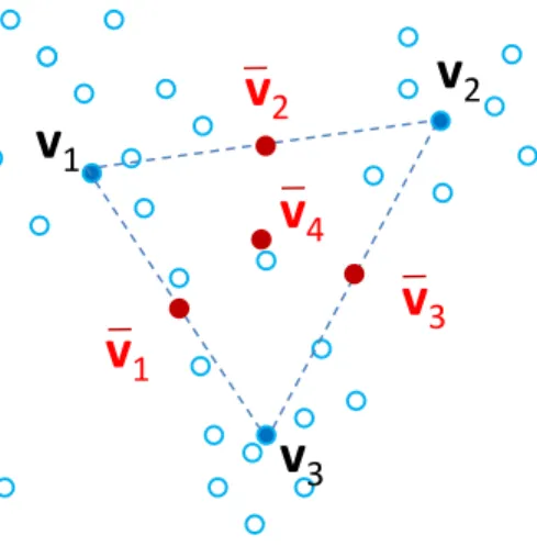
In contrast to EVCLUS, the Evidential c-means algorithm (ECM) [15] is a prototype-based clustering algorithm, which generalizes the hard and fuzzy c -means (FCM) algorithm. The method is suitable to cluster attribute data. As in FCM, each clusterωk is represented by a prototypevk in the attribute space.

However, in contrast with FCM, each non-empty set of clusters Aj ⊆Ω is also

represented by a prototype vj, which is defined as the center of mass of all

prototypes vk, forωk ∈Ak (Figure 3). Formally,

vj = 1 cj c X k=1 skjvk, (7)

where cj =|Aj| denotes the cardinality ofAj, andskj= 1 if ωk ∈Aj,skj = 0

otherwise.

v

1

v

2

v

3

v

1

v

2

v

3

v

4

Fig. 3.Representation of sets of clusters by prototypes in the ECM algorithm.

Let∆ij denote the distance between a vector xi and prototype vj, and let

the distance between any vectorxiand the empty set by defined as a fixed value

δ. The ECM algorithm is based on the idea thatmij =mi(Aj) should be high if

vj, then mi∅ = mi(∅) should be large. Such a configuration of mass functions

and prototypes can be achieved by minimizing the following cost function,

JECM(M, V) = n X i=1 X {j|Aj6=∅,Aj⊆Ω} cαjm β ij∆ 2 ij+ n X i=1 δ2mβ_i∅, (8) subject to X {j|Aj⊆Ω,Aj6=∅} mij+mi∅= 1 ∀i= 1, n, (9)

whereMis the credal partition andV = (v1, . . . ,vc) is the matrix of prototypes.

This cost function depends on three coefficients:β controls the hardness of the evidential partition as in the FCM algorithm; δ controls the amount of data considered as outliers, as in the Dav´e’s Noise Clustering algorithm [5]; finally parameterαcontrols the specificity of the evidential partition, larger values of

αpenalizing subsets of clusters with large cardinality.

As in FCM, the minimization of the cost functionJECM can be achieved by

alternating two steps: (1) minimizeJECM(M, V) with respect toMfor fixedV,

and (2) minimize JECM(M, V) with respect toV for fixed M. The first step is

achieved by the following update equations,

mij= c−_jα/(β−1)∆−_ij2/(β−1) P Ak6=∅c −α/(β−1) k ∆ −2/(β−1) ik +δ−2/(β−1) , (10)

fori= 1, . . . , nand for allj such thatAj6=∅, and

mi∅= 1−

X

Aj6=∅

mij, (11)

fori= 1, . . . , n. The second step implies solving a system of the formHV =B, whereB is the matrix of sizec×pwith general term

Blq = n X i=1 xiq X Aj3ωl cα_j−1mβ_ij (12)

andH the matrix of sizec×c given by:

Hlk= X i X Aj⊇{ωk,ωl} cα_j−2mβ_ij. (13)

We can observe that Eqs (10)-(11) define an evidential classifier: given the matrixV of prototypes, they make it possible to compute a mass function for any new instance. The prototype-updating step can then be seen as a training phase, where the classifier is fitted to the data. ECM can thus be seen as a decision-directed clustering algorithm.

The Relational Evidentialc-Means (RECM), a version of ECM for dissim-ilarity data, was introduced in [16]. In this version, we assume that the data

consist in a square matrix D = (dij) of dissimilarities between n objects, so

that ECM cannot be used directly. However, if we assume the dissimilaritiesdij

to be metric, i.e., to be squared Euclidean distances in some attribute space, we can still compute the distances ∆ij in (8) without explicitly computing the

vectorsxiandvk, which allows us to find a credal partitionMminimizing (8).

Although the convergence of RECM is not guaranteed when the dissimilarities are not metric, the algorithm has been shown to be quite robust to violations of this assumption.

3.2 EK-NNclus

The EK-NNclus algorithm [8] is another decision-directed clustering procedure based on the evidentialk-nearest neighbor (EK-NN) rule [6]. The EK-NN rule works as follows. Consider a classification problem in which an object ohas to be classified in one ofc groups, based on its distances tonobjects in a dataset. Let Ω = {ω1, . . . , ωc} be the set of groups, and dj the distance between the

object to be classified and object oj in the dataset. The knowledge that object

o is at a distance dj from oj is a piece of evidence that can be represented by

the following mass function onΩ,

mj({ωk}) =ujkϕ(dj), k= 1, . . . , c (14a)

mj(Ω) = 1−ϕ(dj), (14b)

where ϕ is a non-increasing mapping from [0,+∞) to [0,1], and ujk = 1 if oj

belongs to class ωk, ujk = 0 otherwise. In [6], it was proposed to choose ϕ as

ϕ(dj) =α0exp(−γdj) for some constantsα0 andγ. Denoting byNK the set of

indices of the K nearest neighbors of object o is the learning set, the K mass function mj, j ∈ NK are then combined by Dempster’s rule [20] to yield the

combined mass function

m= M

j∈NK

mj. (15)

A decision can finally be made by assigning objectoto the classωkwith the

high-est plausibility. We can remark that, to make a decision, we need not compute the combined mass functionmexplicitly. The contour functionpljcorresponding

tomj in (14) is

plj(ω`) = (1−ϕ(dj))1−uj`, (16)

for`= 1, . . . , c. The combined contour function is thus

pl(ω`)∝

Y

j∈NK

(1−ϕ(dj))1−uj`, (17)

for`= 1, . . . , c. Its logarithm can be written as

lnpl(ω`) = n

X

j=1

whereCis a constant, andwj =−ln(1−ϕ(dj)) ifj∈NK, andwj= 0 otherwise.

The EK-NNclus algorithm implements a decision-directed approach, using the above EK-NN rule as the base classifier. We start with a matrixD= (dij)

of dissimilarities between nobjects. To initialize the algorithm, the objects are labeled randomly (or using some prior knowledge if available). As the number of clusters is usually unknown, it can be set to c =n, i.e., we initially assume that there are as many clusters as objects and each cluster contains exactly one object. If n is very large, we can give c a large value, but smaller than n, and initialize the object labels randomly. As before, we define cluster-membership binary variables uik as uik = 1 is object oi belongs to cluster k, and uik = 0

otherwise. An iteration of the algorithm then consists in updating the object labels in some random order, using the EKNN rule. For each object oi, we

compute the logarithms of the plausibilities of belonging to each cluster (up to an additive constant) using (18) as

sik=

X

j∈NK(i)

wijujk, k= 1, . . . , c, (19)

where wij =−ln(1−ϕ(dij)) and NK(i) is the set of indices of the K nearest

neighbors of object oi in the dataset. We then assign object oi to the cluster

with the highest plausibility, i.e., we update the variablesuik as

uik=

(

1 ifsik= maxk0s_ik0,

0 otherwise. (20)

If the label of at least one object has been changed during the last iteration, then the objects are randomly re-ordered and a new iteration is started. Other-wise, we move to the last step described below, and the algorithm is stopped. We can remark that, after each iteration, some clusters may have disappeared. To save computation time and storage space, we can update the number c of clusters, renumber the clusters from 1 toc, and change the membership variables

sik accordingly, after each iteration. After the algorithm has converged, we can

compute the final mass functions

mi=

M

j∈NK(i)

mij, (21)

fori= 1, . . . , n, where eachmij is the following mass function,

mij({ωk}) =ujkϕ(dij), k= 1, . . . , c (22a)

mij(Ω) = 1−ϕ(dij). (22b)

As compared to EVCLUS, EK-NNclus yields a credal partition with simpler mass functions, whose focal sets are the singletons and Ω. A major advantage of EK-NNclus is that it does not require the number of clusters to be fixed in advance. Heuristics for tuning the two parameters of the algorithm, K and γ, are described in [8]. Also, EK-NNclus is applicable to non-metric dissimilarity data.

3.3 EVCLUS

The EVCLUS algorithm [9,10] applies some ideas from Multidimensional Scaling (MDS) [4] to clustering. LetD= (dij) be ann×ndissimilarity matrix, wheredij

denotes the dissimilarity between objectsoi andoj. To derive a credal partition

M= (m1, . . . , mn) fromD, we assume that the plausibilityplij that two objects

oi and oj belong to the same class is a decreasing function of the dissimilarity

dij: the more similar are two objects, the more plausible it is that they belong

to the same cluster. Now, it can be shown [10] that the plausibilityplij is equal

to 1−κij, where κij is the degree of conflict between mi and mj. The credal

partition M should thus be determined in such a way that similar objects oi

and oj have mass functions mi and mj with low degree of conflict, whereas

highly dissimilar objects are assigned highly conflicting mass functions. This can be achieved by minimizing the discrepancy between the pairwise degrees of conflict and the dissimilarities, up to some increasing transformation. In [10], we proposed to minimize the following stress function,

J(M) =ηX i<j (κij−δij)2, (23) where η = P i<jδ 2 ij −1

is a normalizing constant, and the δij = ϕ(dij) are

transformed dissimilarities, for some fixed increasing function ϕ from [0,+∞) to [0,1]. A suitable choice for ϕ is a soft threshold function, such as ϕ(d) = 1−exp(−γd2_{), whereγ is a user-defined parameter. A heuristic for fixing γ is} described in [10]. The stress function (23) by the Iterative Row-wise Quadratic Programming (IRQP) [10, 21]. The IRQP algorithm consists in minimizing (23) with respect to each mass functionmiat a time, leaving the other mass functions

mj fixed. At each iteration, we thus solve

min

mi

X

j6=i

(κij−δij)2, (24)

such thatmi(A)≥0 for any A⊆Ω andPA⊆Ωm(A) = 1, which is a linearly

constrained positive least-square problem that can be solved efficiently. We can remark that this algorithm can be seen as a decision-directed procedure, where each object oi is classified at each step, using its distances to all the other

objects. The IRQP algorithm has been shown to be much faster than the gradient procedure, and to reach lower values of the stress function.

A major drawback of the EVCLUS algorithm as originally proposed in [9] is that it requires to store the whole dissimilarity matrix D, which precludes its application to very large datasets. However, there is usually some redundancy in a dissimilarity matrix. In particular, if two objectso1ando2are very similar, then any object o3 that is dissimilar fromo1 is usually also dissimilar fromo2. Because of such redundancies, it might be possible to compute the differences between degrees of conflict and dissimilarities, for only a subset of randomly sampled dissimilarities. More precisely, letj1(i), . . . , jk(i) bekintegers sampled

at random from the set {1, . . . , i−1, i+ 1, . . . , n}, for i= 1, . . . , n. LetJk the

following stress criterion,

Jk(M) =η n X i=1 k X r=1 (κi,jr(i)−δi,jr(i)) 2_{, (25)}

where, as before,η is a normalizing constant. Obviously, J(M) is recovered as a special case when k=n−1. However, in the general case, the calculation of

Jk(M) requires onlyO(nk) operations. Ifkcan be kept constant asnincreases,

or, at least, if k increases slower than linearly with n, then significant gains in computing time and storage requirement could be achieved [10].

4

Conclusions

The notion of credal partition, as well as its relationships with alternative cluster-ing paradigms have been reviewed. Basically, each of the alternative partitional clustering structures (i.e., hard, fuzzy, possibilistic and rough partitions) corre-spond to a special form of the mass functions within a credal partition. A credal partition can be transformed into a simpler clustering structure for easier inter-pretation. Recently, evidential clustering has been successfully applied in various domains such as machine prognosis [19], medical image processing [13, 14] and analysis of social networks [22]. Three main algorithms for generating credal partitionsand implemented in the R packageevclusthave been reviewed. Each of these three algorithms have their strengths and limitations, and the choice of an algorithm depends on the problem at hand. Both ECM and EK-NN are very efficient for handling attribute data. EK-NN has the additional advantage that it can determine the number of clusters automatically, while EVCLUS and ECM produce more informative outputs (with masses assigned to any subsets of clusters). EVCLUS was shown to be very effective for dealing with non metric dissimilarity data, and the recent improvements reported in [10] make it suitable to handle very large datasets. Methods for exploiting additional knowledge in the form of pairwise constraints have been studied in [1, 2], and the problem of handling a large number of clusters has been addressed in [10].

In future work, it will be interesting to performed detailed comparative ex-periments with these algorithms using a wide range of attribute and dissimilarity datasets. Such a study will require the definition of performance indices to mea-sure the fit between a credal partition and a hard partition, or between two credal partition. This approach should provide guidelines for choosing a suitable algorithm, depending on the characteristics of the clustering problem.

References

1. V. Antoine, B. Quost, M.-H. Masson, and T. Denoeux. CEVCLUS: evidential clustering with instance-level constraints for relational data. Soft Computing, 18(7):1321–1335, 2014.

2. V. Antoine, B. Quost, M.-H. Masson, and T. Denoeux. CECM: Constrained eviden-tial c-means algorithm. Computational Statistics & Data Analysis, 56(4):894–914, 2012.

3. J. Bezdek. Pattern Recognition with fuzzy objective function algorithm. Plenum Press, New-York, 1981.

4. I. Borg and P. Groenen. Modern multidimensional scaling. Springer, New-York, 1997.

5. R. Dav´e. Characterization and detection of noise in clustering.Pattern Recognition

Letters, 12:657–664, 1991.

6. T. Denœux. A k-nearest neighbor classification rule based on Dempster-Shafer theory. IEEE Trans. on Systems, Man and Cybernetics, 25(05):804–813, 1995. 7. T. Denœux. evclust: Evidential Clustering, 2016. R package version 1.0.2. 8. T. Denœux, O. Kanjanatarakul, and S. Sriboonchitta. EK-NNclus: a clustering

procedure based on the evidentialk-nearest neighbor rule. Knowledge-based Sys-tems, 88:57–69, 2015.

9. T. Denœux and M.-H. Masson. EVCLUS: Evidential clustering of proximity data.

IEEE Trans. on Systems, Man and Cybernetics B, 34(1):95–109, 2004.

10. T. Denœux, S. Sriboonchitta, and O. Kanjanatarakul. Evidential clustering of large dissimilarity data. Knowledge-based Systems, 106:179–195, 2016.

11. D. Dubois and H. Prade. Consonant approximations of belief measures.

Interna-tional Journal of Approximate Reasoning, 4:419–449, 1990.

12. R. Krishnapuram and J. Keller. A possibilistic approach to clustering. IEEE

Trans. on Fuzzy Systems, 1:98–111, May 1993.

13. B. Lelandais, S. Ruan, T. Denœux, P. Vera, and I. Gardin. Fusion of multi-tracer PET images for dose painting. Medical Image Analysis, 18(7):1247–1259, 2014. 14. N. Makni, N. Betrouni, and O. Colot. Introducing spatial neighbourhood in

evi-dential c-means for segmentation of multi-source images: Application to prostate multi-parametric MRI. Information Fusion, 19:61–72, 2014.

15. M.-H. Masson and T. Denoeux. ECM: an evidential version of the fuzzy c-means algorithm. Pattern Recognition, 41(4):1384–1397, 2008.

16. M.-H. Masson and T. Denœux. RECM: relational evidential c-means algorithm.

Pattern Recognition Letters, 30:1015–1026, 2009.

17. G. Peters. Is there any need for rough clustering? Pattern Recognition Letters, 53:31–37, 2015.

18. G. Peters, F. Crespo, P. Lingras, and R. Weber. Soft clustering: fuzzy and rough approaches and their extensions and derivatives.International Journal of

Approx-imate Reasoning, 54(2):307–322, 2013.

19. L. Serir, E. Ramasso, and N. Zerhouni. Evidential evolving Gustafson-Kessel al-gorithm for online data streams partitioning using belief function theory.

Interna-tional Journal of Approximate Reasoning, 53(5):747–768, 2012.

20. G. Shafer.A mathematical theory of evidence. Princeton University Press, Prince-ton, N.J., 1976.

21. C. J. ter Braak, Y. Kourmpetis, H. A. Kiers, and M. C. Bink. Approximating a similarity matrix by a latent class model: A reappraisal of additive fuzzy clustering.

Computational Statistics & Data Analysis, 53(8):3183–3193, 2009.

22. K. Zhou, A. Martin, Q. Pan, and Z.-G. Liu. Median evidential c-means algorithm and its application to community detection. Knowledge-Based Systems, 74(0):69– 88, 2015.