Instance-level Semantic Segmentation by Deep Normalized Cuts

(1)

I

NSTANCE

-

LEVEL

S

EMANTIC

S

EGMENTATION BY

D

EEP

N

ORMALIZED

C

UTS

ALEXANDER

DAVIDSON

Master’s thesis 2017:E55 Faculty of Engineering

Centre for Mathematical Sciences Mathematics

CE

N

T

RU

M

S

CI

E

N

T

IA

RU

M

A

T

H

E

M

A

T

ICA

RU

M

(2)

(3)

Abstract

Instance-level semantic segmentation refers to the task of assigning each pixel in an image an object class and an instance identity label. Due to its complexity, this problem has received little attention by the research community in the past. However, owing to the recent successes of deep learning technology, solving it suddenly seems possible.

Starting from an initial pixel-level semantic segmentation, we combine ideas from spectral clustering and deep learning to investigate the suitability of using normalized cuts for additional instance-level segmentation. Specifically, the similarity matrix on which cuts are based is learned from examples using a convolutional network. We use the Cityscapes dataset for urban street scene understanding to train our deep normalized cuts model to segment individual cars. When using the ground truth number of instances to help deter-mine the correct number of cuts, our method attains almost twice the performance of our connected components baseline.

(4)

(5)

Acknowledgements

The author would like to thank Prof. Dr. Cristian Sminchisescu for suggesting the topic of this thesis, for providing access to a GPU, and for offering some guidance along the way.

(6)

(7)

Introduction

1.1 Objective

Object recognitioncomes in many forms, two of the most popular beingobject detection

andpixel-level semantic segmentation(Hariharan et al., 2014). In object detection, the task is to provide a tight, rectangular bounding box around each object of a particular class in an image. Typically, a predicted bounding box is deemed correct if it overlaps with a ground truth box by50%or more, and the performance of an algorithm is evaluated based on itsprecision(the fraction of correctly predicted boxes) andrecall(the fraction of correct boxes reported). While an object detection system attempts to find and estimate the spatial location of each instance of a class, the bounding boxes allow the detected objects to be localized only very coarsely.

Pixel-level semantic segmentation requires each pixel in an image to be assigned to one of several semantic classes. The standard measure used to assess the performance of an algorithm concerned with pixel-level segmentation is theintersection over unionmetric, which for each class computes the fraction of intersecting pixels between the predicted and ground truth segments. The pixel-level segmentation task lacks the notion of object instances. While an algorithm may successfully report all “car” pixels in an image, it does not indicate how many cars there are, nor does it explicitly predict the precise spatial extent of any of those cars.

Intersecting these two forms of object recognition naturally leads to the problem of

instance-level semantic segmentation. Here, the task is to detect all object instances of a class in an image and, for every instance, indicate what pixels belong to it. The performance measure used for this task is analogous to the one used for object detection. Compared to object detection and pixel-level semantic segmentation, the problem of instance-level semantic segmentation requires a more complex, arguably more useful output.

(10)

The objective of this thesis is to investigate a particular approach for solving the prob-lem of instance-level semantic segmentation. Starting with an algorithm that performs pixel-level semantic segmentation, the goal is to further partition the pixels of a certain class into individual object instances using the method ofnormalized cuts(Shi and Malik, 2000). Following the work of Bach and Jordan (2006) and Ionescu et al. (2015),features

on which those cuts are based are to be learned throughdeep learning, using a convolu-tional neural network. We refer to the resulting method asdeep normalized cuts(DNC).

1.2 State of the Art

The recent resurrection of deep learning, in part due to today’s availability of large-scale datasets and the advent of general purpose GPU computing, has stimulated great progress in many fields, including that of computer vision. These days, methods that exploit neural network technology in one way or another dominate leaderboards of many computer vision benchmarks. Deep learning research is very active, and advances are made at a fast pace. As a matter of fact, several of the methods mentioned below have been proposed during the writing of this thesis.

Many recent systems that perform instance-level semantic segmentation make use of the region-based convolutional neural network (R-CNN) object detection framework (Girshick et al., 2014). R-CNN consists of three modules. First, class-agnosticregion pro-posalsthat define the set of candidate detections are generated throughselective search

(Uijlings et al., 2013). Secondly, a convolutional neural network extracts a fixed-length feature vector for each (warped) region. Lastly, a set of class-specific, linear support vector machines (SVMs) are used for classification. During inference, some2,000 re-gion proposals are generated. Non-maximum suppressionis used to discard sub-optimal bounding boxes, and the SVMs are used to predict the semantic class of each box.

Fast R-CNN(Girshick, 2015) makes some modifications to R-CNN that lead to im-provements in terms of both speed and accuracy. DeepMask(Pinheiro et al., 2015) learn to propose candidate object segments, which are then classified by Fast R-CNN.

Faster R-CNN(Ren et al., 2015) generates region proposals using aregion proposal network(RPN), and is currently the leading framework in several object detection bench-marks. Mask R-CNN(He et al., 2017) achieve state-of-the-art performance by adapting Faster R-CNN for instance-level semantic segmentation. In parallel to performing bound-ing box regression and classification, Mask R-CNN additionally predicts a binary object mask. This is different from many other recent systems, in which classification is depen-dent on mask predictions.

(11)

Another successful method for instance-level semantic segmentation is proposed by Li et al. (2016). It combines the segment proposal system of Dai, He, Li, Ren and Sun (2016) with the object detection system of Dai, Li, He and Sun (2016). The common idea in these systems is to detect instances from position-sensitive feature maps that jointly consider object classes, bounding boxes, and segmentation masks, making their implementations fast.

Some methods based on object detectors may assign multiple instances to the same pixel. A conceptually different way of performing instance-level semantic segmentation, that resolves this problem, is to instead begin with a pixel-level semantic segmentation, then attempt to further partition the segments of a given class into individual object in-stances. The pyramid scene parsing network (PSPNet) of Zhao et al. (2016) demon-strates state-of-the-art performance on several pixel-level segmentation benchmarks. Start-ing from an image’s pixel-level semantic segmentation, as produced by PSPNet, Bai and Urtasun (2016) combine intuitions from the classical watershed transform and modern deep learning to produce an energy map of the image, where object instances are represented as energy basins. A cut at a single energy level yields connected components that correspond to object instances. Arnab and Torr (2017) use an initial pixel-level semantic segmentation module and cues from an object detector to feed an instance-aware subnetwork that uses an end-to-end conditional random field to predict instances. Both of these methods prove successful at performing instance-level semantic segmentation.

The mechanism used by human beings to infer object segments is arguably more sim-ilar to the above methods that start off with object detection. Be that as it may, this thesis follows the latter approach and attempts to carve out individual object instances from pixel-level segmentations. (It does, however, not attempt to compete with current state of the art methods.)

1.3 Outline

The remainder of this thesis is organized as follows. Chapter 2 begins with a brief intro-duction to the field of machine learning, then moves on to discuss aspects of deep learning that are important for understanding deep normalized cuts. The primary reference for this chapter is the recent textbook of Goodfellow et al. (2016). Most claims not explicitly cited here can be traced back to this textbook. Chapter 3 is concerned with image partitioning through normalized cuts, and how features suitable for normalized cuts can be learned from data. Chapter 4 first describes the dataset and implementation used for experimentation, then presents the result of applying the latter on the former. Chapter 5 concludes.

(12)

(13)

Chapter 2

Deep Learning

2.1 Machine Learning

2.1.1 Learning Algorithms

Amachine learning algorithmis an algorithm that can learn from data. The following definition, which is due to Mitchell (1997), is often used.

A computer program is said to learn from experienceE with respect to some class of tasksT and performance measureP, if its performance at tasks inT,

as measured byP, improves with experienceE.

Given this definition, learning is not the task. Instead, learning refers to the process of acquiring the ability to perform the task. Tasks are commonly described in terms of how the algorithm should process anexample, which is a collection offeaturesassociated with some object or event. In the case of an image, the features could be the intensity values of the image’s pixels.

The performance measure offers a means to quantitatively measure the abilities of a machine learning algorithm. It is specific to the task being solved. In order to assess how aptly an algorithm will work once deployed in the real world, we are typically interested in how well it performs on previously unseen data. To this end, the performance is not evaluated on the data used totrainthe algorithm, but on a separatetest set.

Machine learning algorithms can be coarsely grouped asunsupervisedorsupervised

by the kind of experience they are provided during training. In essence, unsupervised learn-ing involves observlearn-ing examplesxof a random vectorxand trying to learn the probability distributionpx(x), or some useful properties thereof, whereas the supervised learning case

additionally involves observing instancesyof an associated targety, and learning to pre-dictyfromx, typically by estimatingpy(y|x=x).

(14)

2.1.2 Generalization

The central challenge in machine learning lies in designing algorithms that perform well on unobserved data, an ability calledgeneralization. During training, some measure of

training errorcan typically be computed. Minimizing this error is simply an optimization problem. What sets machine learning apart from optimization is that we also want the

generalization errorto be small. The generalization error is defined as the expected value of the error on a new input, taken over possible inputs drawn from the distribution of inputs that we expect to encounter in practice. It is usually approximated by the average error on the test set examples.

If the training and test sets are gathered arbitrarily, there is no reason to expect the test error to be affected when only the training set is observed during training. Some assumptions about how the data is collected are needed. The training and test data are generated by a probability distribution over datasets called thedata generating process. If we assume that the examples in each dataset are independent from each other, and that the two datasets are identically distributed, drawn from the same probability distribution, then we may describe the data generating process with a probability distribution over a single example. This shared data generating distribution is then used to generate every training and test example. It follows that the expected training error of a randomly selected model equals the expected test error of that model, and, in turn, that machine learning algorithms can generalize well from a finite set of training examples.

In machine learning, we want both the training error and the gap between the training and test errors to be small. These concerns correspond to two principal machine learn-ing challenges, calledunderfittingandoverfitting. Underfitting refers to the situation in which the model fails to obtain a small enough training error. If the training error is small but the test error is not, overfitting has occurred.

By adjusting thecapacity of the model, we can control how likely it is to underfit or overfit the training data. A model’s capacity may be viewed as its ability to fit a wide range of functions. A model with low capacity may not be able to fit the training set. A model with high capacity is prone to overfit the training set by capturing specific properties of the training data that do not fully generalize to the test data.

The capacity of a machine learning algorithm can be controlled via the choice of its

hypothesis space, which is the set of functions from which it selects the solution. Adding more complex functions to the hypothesis space increases the model capacity. The model describes which family of functions the learning algorithm may chose from when adjusting its parameters in order to lower the training error. This is referred to as therepresentational

(15)

Typically, the learning algorithm simply settles on a function that results in a small enough training error. As a consequence, theeffectivecapacity of the model may be less than the representational capacity of the model family.

2.1.3 The No Free Lunch Theorem

Theno free lunch theoremfor machine learning (Wolpert, 1996) states that every classi-fication algorithm will attain the same error rate on previously unseen data, when averaged across every possible data generating distribution. The meaning of this is that no machine learning algorithm is universally any better than any other. Luckily, if taking into consid-eration only the types of probability distributions we expect to confront in practice, then we can build algorithms that perform well on those distributions. The ambition of machine learning research is to understand what machine learning algorithms work well on data drawn from data generating distributions that are relevant in the real world, and not to find a universal machine learning algorithm.

2.1.4 Regularization

A machine learning algorithm is designed to work well on a particular task by incorporating certain preferences into it. Apart from altering the representational capacity of the model, we can also give a learning algorithm a preference for some solutions in its hypothesis space to others. While all solutions are allowed, an unpreferred solution must fit the training data significantly better than a preferred solution in order to be selected.

Preferences can be expressed in different ways. These different ways are collectively known asregularization, which is any modification made to a learning algorithm that is intended to lower its generalization error but not its training error. Regularization is an important topic in machine learning, and just as with the learning algorithm itself, what kind of regularization to use depends on the nature of the particular task being solved.

2.1.5 Hyperparameters

In addition to the model parameters being learned, a machine learning algorithm usually hashyperparametersthat influence its behavior. Sometimes a parameter is chosen to be a hyperparameter because it is difficult to optimize, but often a parameter must be a hyper-parameter because it is inappropriate to learn it from the training data. This includes all hyperparameters that control model capacity, because learning such parameters inevitably results in the highest possible capacity being selected, which might cause overfitting.

(16)

To help us choose appropriate values for the hyperparameters, we construct a valida-tion setof examples that are not used during training. It is important that the examples in the test set are in no way used to make decisions about a model, including the associ-ated hyperparameters. To this end, the training data is split into two disjoint subsets. One of these, also referred to as the training set, is used to learn the parameters of the model, whereas the other subset, the validation set, is used to approximate the generalization error during or after training, which allows for the hyperparameters to be tuned. The validation set error is likely to underestimate the generalization error, since the validation set is used to adjust the hyperparameters. However, it usually does so by a smaller amount than does the training set error. Upon the completion of hyperparameter optimization, the generalization error may be estimated using the test set.

2.1.6 Designing a Machine Learning Algorithm

A typical machine learning algorithm can be described as a combination of a dataset, a cost function to minimize, an optimization scheme, and a model. These building blocks can be interchanged mostly independently of each other, which results in a wide range of possible algorithms.

The cost function usually includes one or more terms that cause the learning process to perform statistical estimation. It may also include additional terms, such as a regularizer. If the model is nonlinear, most cost functions cannot be optimized in closed form, but demand the employment of an iterative, numerical optimization procedure, such as gradient descent.

2.2 Deep Feedforward Networks

Deep feedforward networks, orfeedforward neural networks, are the prototypical deep learning models. The goal of a deep feedforward network is to approximate some function mapping y = f(x). It does so by defining an approximate mappingy _⇡ fˆ(x;⇡) and learning the values of the parameter vector⇡that result in the best approximation off.

Deep feedforward networks are called “feedforward” because information flows from the inputx, through the computational operations that define_fˆ_{, before it reaches the output} y. There is no feedback loop that connects the output back to the model.

Deep feedforward networks are called “networks” because these models are typically constructed by composing together many different functions. For instance,_fˆ_{may be} com-posed of N chained functions to form fˆ(x) =⇣fˆ(N) fˆ(N 1) _{· · ·} fˆ(1)⌘(x). Then,

ˆ

f(1) _{is called the first} _layer_, _fˆ(2) _{the second layer, and so on. The final layer of a} feed-forward network is called theoutputlayer, and the length of the chain corresponds to the

(17)

depthof the network, hence the termdeep learning.

Each training example(x,y)provides a noisy, approximate example of howf acts. A training example specifies that the output layer should produce a quantity close toywhen xis fed into the model. However, the behavior of the intermediate layers is left unspecified by the training data, and the learning algorithm is left to self decide how to use those layers to produce the prescribed output. Since the training data does not show the desired output for any of these layers, these layers are calledhidden.

Finally, these models are called “neural” because they draw some inspiration from neu-roscience. Each hidden layer of the network may be seen as a set ofunitsthat operate in parallel, with each unit playing a role similar to that of a biological neuron, in the sense that it receives input from many other units and then computes its own activation value. How-ever, the goal of neural network research is not to perfectly model the brain. It is perhaps best to view feedforward networks as function approximators built to achieve statistical generalization, that draw some insights from what is known about the brain.

2.2.1 Interpretation

Linear models are simple and can be fit efficiently, either in closed form or through convex optimization. However, their capacity is restricted to linear functions, which means that they cannot capture the interaction between any two input variables.

We can extend linear models to represent nonlinear functions of the inputxby applying the linear model not to x itself, but to a transformed version (x) ofx. The nonlinear mapping may be thought of as providing a set of features describingx, or giving a new

representationofx. There are different ways to choose . The strategy of deep learning is to learn it from examples. Using this strategy gives a modely= ˆf(x;⇡,w) =wT ₍_x_;_⇡₎_, where the parameter vector⇡is used to learn , and the weightswmap (x)to the desired output. This is an example of a feedforward network, with defining a hidden layer.

The nonlinear transformation used to describe the features is commonly formed as an affine transformation controlled by learned parameters, followed by a fixed, nonlinear

activation function. That is to say, (x) = a(Wx+b), with weightsW and biasesb. The activation functionais usually applied element-wise. Today, the standard activation function is therectified linear unit, or ReLU, defined as a(z) = max(z, 0). Although nonlinear, the rectified linear unit is close to linear in the sense that it consists of two linear pieces, and thus keeps some of the properties that make linear models easy to optimize with gradient-based methods, as well as some of the properties that make linear models generalize well. The fact that the rectified linear unit is non-differentiable at the origin may seem like a problem in the context of gradient-based learning. However, in practice, we do

(18)

not expect training to reach a point where the gradient is exactly zero, which reduces this fact to a technical detail.

What type of output unit to use depends on the choice of cost function. Any kind of unit used in the output layer can also be used in a hidden layer. An example of an output unit is the so-called softmax unit, which is commonly used as the output unit of a classification network, to represent the probability distribution overK different classes. The softmax function maps an input vector z 2 RK _{into a probability vector that can be} used to represent a categorical distribution. It is defined as

softmax(z)_i = _P_Kexp(zi) j=1exp(zj)

, (2.1)

fori₂_{1, 2,. . .,K_}. The softmax function can be seen as a generalization of the logistic function used to represent the probability distribution over a binary variable.

2.2.2 The Back-propagation Algorithm

In contrast to the linear equation solvers used to train linear regression models, or the con-vex optimization algorithms with global convergence guarantees used to train models such as logistic regression and support vector machines, neural networks are typically trained using iterative, gradient-based optimization schemes that merely drive the cost function to a low value. It is, however, perfectly viable to train also these other models with gradient descent. This is commonly done when the training set is very large. In this sense, train-ing a neural network is not much different from traintrain-ing any other model. Computtrain-ing the gradient is somewhat more involved, but can still be done efficiently and exactly.

The stage during which information flows through the network from input to output is calledforward propagation. During training, forward propagation yields a scalar cost C(⇡), or typically, an approximation thereof. Theback-propagationalgorithm (Rumel-hart et al., 1986) enables information from the cost to then flow backwards through the network in order to compute the gradient.

The back-propagation algorithm refers only to the method of computing the gradient, whereas a separate optimization algorithm is responsible for using the gradient to perform learning. It is not restricted to neural networks, but can in principle be used to compute derivatives of any function for which these are defined. In the context of machine learning, the gradient we most commonly require is the gradient of the cost function with respect to the parameters,r⇡C(⇡).

In calculus, we compute derivatives of functions formed by composing other functions whose derivatives are known using the chain rule. Back-propagation is an algorithm that unfolds the chain rule in an efficient order.

(19)

Letx₂_RN_,_y₂_RM_,_g_:_RN _! _RM_{, and}_h_:_RM _!_R_{. If}_y₌_g₍_x₎_and_z ₌_h₍_y₎_, then @z @xi = M X j=1 @z @yj @yj @xi , (2.2)

fori2{1, 2,. . .,N}. This is equivalent to writing

rxz= ✓ @y @x ◆T ryz, (2.3)

where @y/@x is the M ⇥N Jacobian matrix of g. Thus, the gradient of a variable x can be obtained by multiplying a Jacobian matrix@y/@xby a gradient _ryz. The

back-propagation algorithm carries out such a Jacobian-gradient multiplication for each opera-tion in the network. It is not restricted to work only on vectors, but is applicable to tensors of arbitrary dimensionality. Conceptually, this is the same thing, the only difference being how the numbers are organized.

It is straightforward to derive an algebraic expression for the gradient of a scalar with respect to any computational node in the graph representation of a network using the chain rule. Actually evaluating that expression on a computer requires some extra care. Specif-ically, many subexpressions may appear several times within the overall expression of the gradient, and so decisions about whether to store or recompute these subexpressions need be made. For complicated networks, the same subexpression can appear so many times that a naive implementation of the chain rule becomes infeasible. The back-propagation algorithm reduces the number of common subexpressions without regard to memory by storing intermediate result, a strategy called dynamic programming.

The back-propagation algorithm is just one approach to performing automatic differen-tiation. Other approaches evaluate the subexpressions of the chain rule in different orders. Therefore, the back-propagation algorithm is not the only way, let alone the optimal way of computing the gradient, but is a practical method that currently serves the deep learning community well.

2.2.3 Architecture Design

An important aspect when designing a deep learning system is the choice ofarchitecture, which refers to the structure of the network. This includes how many units different layers should have, and how these layers should be connected to each other. The key architectural considerations for chain-based networks are the depth of the network and the width of each layer. Deep networks can be numerically difficult to optimize, but are typically able to generalize well to the test set using relatively few units per layer. There are few guidelines

(20)

when it comes to architecture design, and the ideal network architecture for a task must be found through experimentation.

2.3 Optimization

2.3.1 Empirical Risk Minimization

In the typical machine learning setting, we are interested in building a system that performs well according to some performance measureP. Sometimes, the very nature ofPmakes it impossible to optimize. In addition,P is evaluated with respect to the test set, which means that we can only target it indirectly. We do this by minimizing some other cost functionC, and hope that doing so will improve performance with respect toP as well.

The cost function can usually be written as an average over the training set, such as C(⇡) =E₍_x_,_y₎_⇠_pdata_ˆ L⇣fˆ(x;⇡),y⌘ (2.4) = 1 N N X i=1 L⇣fˆ⇣x(i);⇡⌘,y(i)⌘, (2.5) whereLis a per-example loss function,fˆ(x;⇡)is the output predicted by the model when the input isx, andpˆdatais theempirical distribution, which puts equal probability mass on

each of theN training examples. In the supervised case,yis the target output. Ideally, we would prefer to minimize the expectation in (2.4) with respect to the true data generating distributionpdata,

R(⇡) =E₍_x_,_y₎_⇠_pdataL⇣fˆ(x;⇡),y⌘, (2.6) which is nothing but the expected generalization error, also known as therisk. If we knew pdata, risk minimization would be a regular optimization problem. However, since we do

not know pdata, but merely have a limited set of training examples, we face a machine

learning problem. To convert this problem back into an optimization problem, we replace the true distribution pdata with the empirical distribution pˆdata and instead minimize the

empirical riskdefined by (2.4). Hopefully, minimizing the average training error will lead to a significant decrease in the true risk as well.

2.3.2 Mini-batch Algorithms

Gradient-based optimization algorithms used in machine learning compute parameter up-dates based on the gradient of the empirical risk with respect to the model parameters. Provided that the cost function decomposes as a sum over the training examples, this

(21)

gra-dient is given by r⇡C(⇡) =E(x,y)⇠pˆdatar⇡L ⇣ ˆ f(x;⇡),y⌘ (2.7) = 1 N N X i=1 r⇡L ⇣ ˆ f⇣x(i);⇡⌘,y(i)⌘. (2.8) Computing this expectation exactly is likely to be very expensive, since it requires evalu-ating the model on each of theN training examples. Fortunately, we can approximate the expectation by using only a small, randomly sampled subset of the training examples.

Optimization algorithms that in each iteration compute the gradient based on the entire training set are traditionally called batch algorithms, whereas algorithms that do so by using only a single example at a time are calledstochastic. Many optimization algorithms used for deep learning use more than one but less than all training examples to perform parameter updates. Such algorithms are referred to asmini-batchalgorithms. An example of a commonly used mini-batch algorithm ismini-batch gradient descent.

What mini-batch size to use for a mini-batch algorithm depends on several factors. Larger mini-batches can estimate the gradient more accurately, but do so with less than linear returns. Smaller mini-batches can have a regularizing effect (Wilson and Martinez, 2003), maybe because of the noise they add to the learning process. The purely stochastic case often results in the lowest generalization error, but training with such a small mini-batch size may require taking very small steps in the direction of the negative gradient to maintain stability due to the high variance in the gradient estimate. This might result in slow convergence, not only due to the small steps themselves, but also because it takes more updates to observe the entire training set. First-order methods that base parameter updates only on the gradient are usually fairly robust and can handle small mini-batch sizes. Second-order methods that, in addition to the Jacobian also use the Hessian matrix, often require much larger mini-batch sizes to be stable.

Computing an unbiased estimate of the expected gradient from a subset of training examples requires that those examples be selected randomly. Moreover, since we want subsequent estimates of the gradient to be independent of each other, subsequent mini-batches should be independent of each other.

One motivation for mini-batch gradient descent is that is follows the gradient of the true risk in (2.6) if no examples are repeated. If both xandy are discrete, (2.6) can be expressed as a sum, R(⇡) =X x X y pdata(x,y)L ⇣ ˆ f(x;⇡),y⌘, (2.9)

(22)

having the exact gradient g=_r⇡R(⇡) = X x X y pdata(x,y)r⇡L ⇣ ˆ f(x;⇡),y⌘. (2.10) A similar result holds for the continuous case. As a consequence of this, an unbiased estimator for the gradient of the risk can be obtained by randomly sampling a mini-batch ofM examples x(1),y(1) ,. . ., x(M),y(M) from the data generating distributionpdata

and computing the gradient of the average per-example loss with respect to the parameters given this mini-batch,

ˆ g= 1 M r⇡ M X i=1 L⇣fˆ⇣x(i);⇡⌘,y(i)⌘. (2.11) Updating the parameter vector⇡in the negative direction ofgˆperforms mini-batch gradi-ent descgradi-ent on the true risk.

This result only holds if no examples are reused. Unless the training set is very large, we usually shuffle it once and then make several passes through it. When making multiple such passes, orepochs, the estimator for the gradient of the risk becomes biased from the second pass and onwards. However, the reduced training error attained from using multiple epochs typically outweighs the harm they cause by widening the gap between training error and test error.

An important property of mini-batch gradient descent is that the amount of computation needed per update does not depend on the size of the training set, allowing for convergence no matter how many training examples there are.

Having computed an estimate of the gradient using (2.11), mini-batch gradient descent updates the parameter vector as⇡ ⇡ gˆ. The hyperparameter is called thelearning rate, and controls the size of the update step. The learning rate is crucial. Taking too large steps may cause the optimization to diverge, whereas taking too small steps could get us stuck in a poor local minimum. If we use the true gradient of the total cost function, then this becomes exactly0when we reach a local minimum, which means that we in this scenario can use a fixed learning rate. However, when using mini-batch gradient descent, the gradient estimate is noisy and will not reach exactly0even when we arrive at a local minimum. To this end, it is important to gradually decrease the learning rate over the course of the optimization process. There exist various policies for doing this. Examples include decreasing the learning rate linearly for some time and then leaving it constant, letting it decrease in a polynomial fashion, or reducing it by some factor whenever the cost seems to stop improving. However, picking the learning rate can be tricky, and most guidance on this subject should be taken with some skepticism.

(23)

An optimization algorithm used in a pure optimization scenario will proceed until a local minimum is reached. However, when used to train a machine learning algorithm, optimization usually halts when overfitting starts to occur. This means that training might stop while the cost function still has large derivatives, which is very different from the pure optimization setting, in which optimization ends when the derivatives become very small.

2.3.3 Momentum

Mini-batch gradient descent is a simple, yet popular optimization algorithm. However, learning with it is sometimes slow. The method ofmomentum(Polyak, 1964) is designed to speed up learning. It does so by accumulating previous gradients in an exponentially decaying moving average, and continuing to partially move in their direction.

The name momentum is due to a physical analogy, in which the negative gradient is a force that moves a particle through parameter space as governed by Newton’s laws of motion. In physics, momentum is defined as mass times velocity. The momentum algorithm assumes unit mass, in which case momentum equals velocity. Formally, the algorithm introduces a momentum parameterpwhich acts as a force in the direction that the parameters currently move through parameter space. A decay rate parameter 2[0, 1) controls the decay of previous gradients. The larger the quotient / , the more impact earlier gradients have on the current direction. Algorithm 2.1 describes mini-batch gradient descent with momentum in more detail.

Algorithm 2.1:Mini-batch gradient descent with momentum. Note that the learning rate is typically set to decrease over the course of iterations.

Require: An initial parameter vector⇡.

Require: A learning rate .

Require: An initial momentump.

Require: A decay rate parameter 2[0, 1).

whilestopping criterion not metdo

Sample a mini-batch x(1)_,_y(1) _,_{. . .}_, _x(M)_,_y(M) _of_M _{training examples.} Estimate the gradient: gˆ _M1 r⇡PM_i=1L

⇣ ˆ

f x(i);⇡ ,y(i)⌘. Update the momentum: p p g.ˆ

Update the parameter vector:⇡ ⇡+p.

(24)

2.3.4 Adaptive Learning Rates

Many times, the cost is highly sensitive to changes in some directions in parameters space but insensitive to changes in others. Momentum can help alleviate this problem to some extent, but does so at the expense of adding another hyperparameter. However, if the directions of sensitivity are somewhat axis-aligned, it may be a good idea to use a separate learning rate for each parameter, and automatically adapt these during training.

Adam(Kingma and Ba, 2014) is one of several optimization algorithms that adapt the learning rate of each model parameter individually. The name “Adam” is a portmanteau of the words “adaptive moments.” Parameter updates are based on estimates of the first and second moments of the gradient, which are its mean and uncentered variance, respectively. The estimates are formed from exponentially decaying averages of past gradients and their squares. The moment vectors are initialized at the origin, which causes their entries to be biased toward zero. To account for these biases, the estimates are biases-corrected. The update step for each parameter is proportional to the first moment, scaled by the inverse of the second moment’s square root. This causes parameters with a large partial derivative of the cost to have a quick decrease in their learning rate, whereas parameters with a small partial derivative of the cost have a comparatively slow decrease in their learning rate. The result of this is greater progress in the directions of parameter space that have low curvature. The Adam algorithm is described more formally in Algorithm 2.2.

2.3.5 Parameter Initialization

Iterative training algorithms for deep models require us to specify an initial point in param-eter space from which to begin the optimization. Training deep models is a difficult task, and the initial point can determine whether the learning algorithm converges at all. When it converges, the initial point has an immediate impact on how quickly it does, and if the final solution corresponds to a point with low or high cost. Moreover, points with similar cost can have drastically different generalization error.

Because optimization of deep models is not well understood, initialization strategies are simple and heuristic. Possibly the only fact known with certainty is that units with the same activation function and inputs should have their parameters initialized differently in order to “break symmetry.” Provided that the optimization algorithm, the cost, and the model are deterministic, these units would otherwise always be updated in the exact same way. A cheap way to circumvent this issue is to initialize the parameters randomly from a high-entropy distribution. This is unlikely to assign any two units the exact same parameters. However, biases are usually not initialized randomly, but rather set to some heuristically chosen constant, such as0. Sometimes we may want to choose the bias to avoid causing

(25)

Algorithm 2.2:Adam. The symbol denotes the Hadamard product, and the formula for updating the parameter vector⇡should be read element-wise.

Require: An initial parameter vector⇡.

Require: A learning rate .

Require: Exponential decay rates 12[0, 1)and 2 2[0, 1)for the moment estimates.

Require: A small constant✏for numerical stability.

Initialize the first-order and second-order moment variables:m1 =0andm2=0. Initialize the time step:t= 0.

whilestopping criterion not metdo

Sample a mini-batch x(1),y(1) ,. . ., x(M),y(M) ofM training examples. Estimate the gradient: gˆ _M1 _r⇡PMi=1L

⇣ ˆ

f x(i)_;_⇡ _,_y(i)⌘_. Increment the time step: t t+ 1.

Update the estimate of the first moment:m1 1m1+ (1 1)g. Update the estimate of the second moment:m2 2m1+ (1 2)g g. Correct for the bias in the first moment:m1 m1/ 1 1t .

Correct for the bias in the second moment:m2 m2/ 1 2t . Update the parameter vector:⇡ ⇡ m1/ pm2+✏ .

end while

too much saturation at initialization. For example, we may set the bias of a hidden unit that uses a rectifier to0.1rather than0to avoid saturating the ReLU at initialization.

2.4 Convolutional Networks

Convolutional networks, or convolutional neural networks, are a specialized kind of neural network that make use of the convolution operator. This makes them suitable for processing data that has a grid-like topology, such as images. Convolutional networks have been highly successful in practical applications. Any network that uses convolution instead of general matrix multiplication in one or more of its layers is a convolutional network.

2.4.1 The Convolution Operator

The convolution between two functionsgandkis defined as

(g⇤k)(t) = Z

Rg(⌧)k(t ⌧)d⌧. (2.12)

In the terminology of convolutional networks,gis called theinput,kthekernel, and the output is commonly referred to as thefeature map. The discrete counterpart of (2.12) is

(26)

defined as (g_⇤k)(t) = 1 X i= 1 g(⌧)k(t i) . (2.13) In deep learning applications, the input and kernel are typically multidimensional ar-rays of data and learnable parameters, respectively. To be able to evaluate an infinite sum-mation on a computer, we assume thatgandkare zero everywhere but the finite number of points for which we store their values.

If the input is a two-dimensional imageI, we typically also want a two-dimensional kernelK, in which case

(I _⇤K)(h,w) =X i

X j

I(i,j)K(h i,w j) . (2.14) Convolution is commutative, which means that

(I ⇤K)(h,w) = (K⇤I)(h,w) =X i

X j

I(h i,w j)K(i,j) . (2.15) The commutative property arises because the kernel has been flipped relative to the input. It is usually not an important property of a neural network implementation. Many software libraries instead implement the related cross-correlation function, which is the same as convolution but without kernel flipping, and call it convolution:

(I _⇤K)(h,w) =X i

X j

I(h+i,w+j)K(i,j) . (2.16) This will cause a learning algorithm to learn kernels that are flipped relative to the kernels it would learn if true convolution was used.

Convolution is a linear operation. This implies that discrete convolution may be viewed as multiplication with a matrix that is constrained to conform to a certain structure. For instance, a one-dimensional kernel can be represented as a Toeplitz matrix, whereas a two-dimensional kernel can be represented as a doubly block circulant matrix. The kernel is typically much smaller than the input, which makes these matrices very sparse.

2.4.2 Motivation

A traditional neural network layer uses matrix multiplication with each element describing the interaction between one input unit and one output unit, which means that every input unit interacts with every output unit. In contrast, convolutional network kernels that are smaller than the input havesparse interactions. For example, a kernel used to detect some feature in an image, such as an edge, can do so using only tens or hundreds of pixels,

(27)

even if the image itself consists of thousands or millions of pixels. With multiple convolu-tional layers, units in the deeper layers may then indirectly interact with a larger portion of the input image, allowing the network to capture complicated interactions between many variables using simple building blocks, each of which interacts only sparsely.

Furthermore, features that can appear anywhere in the image allow us to learn only one set of parameters instead of a separate set of parameters for every input location. This means that each member of a kernel is used at every position of the input, except possibly at some boundary pixels, depending on how we decide to treat the boundary cases. Such

parameter sharing does not apply to traditional, fully connected layers in which each parameter is used only once. As a result, convolutional layers allow us to construct deep networks using relatively few parameters. This reduces the risk of overfitting. The par-ticular form of parameter sharing employed by a convolutional layer makes it invariant to translation. In the case of images, if an object in an image is translated, the representation of that object in the feature map will move accordingly.

2.4.3 Pooling

It is common to arrange a convolutional layer to consist of two or three stages. The first stage performs convolution with many different kernels in parallel to output a linear set of activations. These linear activations are then passed through a nonlinear activation function such as the rectified linear unit. This second stage is sometimes referred to as thedetector

stage. An optional third stage that applies apooling functionmay be used to modify the layer output even further.

A pooling function replaces the output of a layer at a particular position with a summary statistic computed from nearby outputs. Examples of popular pooling functions include

max poolingandaverage pooling, which compute the maximum and average output value within some rectangular neighborhood, respectively.

Pooling helps make the representation become roughly invariant to small translations of the input. Such invariance can be useful in cases where we care more about the potential presence of some feature, and not so much about its exact location.

2.4.4 Practicalities

A convolutional layer typically performs convolution with many different kernels in par-allel. This is because a single kernel can only extract one specific feature, and we usually want each layer to extract many different features. When working with images, the first convolutional layer of a convolutional network might detect edges of various orientation,

(28)

while layers of greater depth learn to combine features detected by preceding layers into features of increasingly sophisticated nature.

Moreover, each location of the input is in general vector-valued. For example, an image might have a red, a green, and a blue intensity at each pixel location. In this setting, we usually think of the input and output of the convolution as being three-dimensional tensors, with one axis indexing into the different channels, and the remaining two axes indexing into each channel’s spatial coordinates. What is more, software implementations commonly operate in mini-batch mode, and thus add a fourth axis that corresponds to the different examples in the mini-batch.

Unless the spatial dimensions of the input to a convolutional layer are padded, the height and width of the output will shrink by one pixel less than the kernel height and width, respectively. The ability to implicitly pad the input is an essential feature of any implementation. Zero-padding is the most common way of expanding the input, but several other padding strategies, such as reflection padding, are sensible. If we actually want to reduce the spatial extent of the feature maps, then a more controlled way of doing so is to modify the so-called strideused by convolutional and pooling layers. The stride defines how much a kernel or pooling window is shifted in between adjacent computations, and thus offers a means to perform sub-sampling of the input. For example, using a stride of two along each spatial coordinate will halve the spatial extent of the output in each direction. This can be an effective way to reduce the amount of computation needed to propagate data through a network.

As a final note, convolutional networks can be used to output a high-dimensional, struc-tured object instead of just a class label for a classification task or a real value for a regres-sion task. This object is usually just a tensorT emitted by a convolutional layer, where entryTk,i,j could, for example, indicate the likelihood of pixel(i,j)belonging to classk. Such a structured output allows us to classify each pixel in the image and draw detailed boundaries around individual objects.

(29)

Chapter 3

Deep Normalized Cuts

3.1 Normalized Cuts

Clusteringrefers to the task of grouping a set of objects in such a way that objects that are grouped together to form a cluster are more similar to each other than to objects that are grouped together to form other clusters, as measured by some notion of similarity.Spectral clusteringis a collective term for clustering techniques that are based on the eigenstructure of asimilarity matrix, comprised of pairwise similarity relations between data points. In the case of image segmentation, data points correspond to features of image pixels.

Assume we have an image consisting of N pixels. Let S be a symmetric N _⇥N similarity matrix such that elementsSij =Sji 0are a measure of the similarity between pixelsiandj, with a large value suggesting that these pixels should belong to the same cluster, and a small value suggesting that they should not. The goal of spectral clustering is to organize the set of pixels into disjoint subsets, such that the similarity within subsets is high, while the similarity across subsets is low.

LetP = _{1, 2,. . .,N_} be an index set of the set of pixels in the image. We wish to partition P into K disjoint, non-empty subsets P1,P2,. . .,PK according to a particular loss function. The loss function we will consider is theK-waynormalized cut(Shi and Malik, 2000; Gu et al., 2001), defined as

ncut(_P1,P2,. . .,PK) = K X k=1 cut(_Pk,P \Pk) cut(Pk,P) , (3.1) with cut(_Pk,P \Pk) = Pi2Pk P

j2P\PkSij, and similarly for cut(Pk,P). Because of the normalizing denominators in (3.1), the K-way normalized cut criterion penalizes un-balanced solutions. This is not the case in the non-normalized setting, which often leads to some clusters containing only a single pixel. Minimizing the inter-cluster similarity

(30)

through (3.1) is equivalent to maximizing the intra-cluster similarity (Shi and Malik, 2000). Hence, both of these criteria can be achieved simultaneously.

Let E ₂ _{0, 1_}N⇥K be an indicator matrix such that Eij equals 1 if pixel i be-longs to part j, and 0 otherwise. Since full knowledge of E entails full knowledge of (_P1,P2,. . .,PK), and vice versa, we will refer toEas a partition. LetD= diag(S1)be the diagonal matrix for which entryDiiis the sum of theithrow ofS. A simple calculation (Gu et al., 2001) reveals that

ncut(E) = K X k=1 ET k(D S)Ek ET k DEk , (3.2)

whereEkdenotes thekth column ofE.

To find a matrixE that minimizes the normalized cut is an NP-hard problem (Shi and Malik, 2000; Meila and Xu, 2003). However, if we embed the problem in the domain of real values, an approximate, discrete solution based on eigenvalue decomposition can be found efficiently.

Bach and Jordan (2006) show that theK-way normalized cut lossncut(E) is equal to K trace QTD 1/2SD 1/2Q , for any matrix Q ₂ RN⇥K that (i) has orthonor-mal columns and (ii) is such that the columns of D 1/2_Q _{are proportional to the} corre-sponding columns ofE. Removing the latter constraint yields a tractable relaxation whose solutions involve the eigenstructure of_S˜ ₌_D 1/2_SD 1/2_{. Consider the} eigendecompo-sition_S˜ ₌_U_⇤_UT_{, where the eigenvalues on the diagonal of}_⇤_{are ordered in descending} order. It follows from Ky-Fan’s theorem (Overton and Womersley, 1993) that the maxi-mum oftrace QT_SQ˜ _{is equal to the sum of the}_K _{largest eigenvalues of}_S˜_{, and that the} maximum is attained for all Q of the form Q = U1:KA, where U1:K 2 RN⇥K is any orthonormal basis of theK-dimensional principal subspace ofS˜, or, in other words, the columns ofU1:Kare the eigenvectors associated with theKlargest eigenvalues ofS˜, and Ais any orthogonal matrix inRK⇥K_{. Naturally, the solution found via this relaxation will} in general not fulfill criterion (ii), which means that it must be projected back to the set of allowed solutions.

The set of matricesRthat correspond to a partition defined byEand satisfy constraints (i) and (ii) are of the formR=D1/2E ETDE 1/2B, whereB2RK⇥K_{is an arbitrary} orthogonal matrix (Bach and Jordan, 2006).

Since bothQ andR are defined up to an orthogonal matrix, it makes sense to try to align the subspace spanned by the columns ofQwith the subspace spanned by the columns ofR. A common way to compute the distance between subspaces is to compare the Frobe-nius norm between the orthogonal projection operators onto those subspaces (Golub and Van Loan, 2012). Note that such a metric is invariant to permutations of the cluster indices.

(31)

The orthogonal projection operators onto the subspaces spanned by the columns ofQand Rare

⇧Q=QQT =U1:KU1:KT (3.3) and

⇧R =RRT =D1/2E ETDE 1ETD1/2, (3.4)

respectively. Measuring the Frobenius norm between these projectors gives rise to the loss function L1(S,E) = 1 2k⇧Q ⇧Rk 2 F (3.5) = 1 2 U1:KU T 1:K D1/2E ETDE 1 ETD1/2 2 F. (3.6) Bach and Jordan (2006) note that if the rank of the similarity matrixSis equal toK, then L1 is equal to theK-way normalized cut,ncut(E).

By construction,U_1:KT U1:K = I. Additional normalization of the rows of U1:K has proved beneficial in clustering applications (Ng et al., 2001). This can be seen by consider-ing the ideal settconsider-ing, in which the similarity is strictly positive for pixels that should belong to the same cluster, and zero otherwise. Then, the eigenvalue1of the matrixS˜has mul-tiplicityK, andD1/2Eis an orthonormal basis of theK-dimensional principal subspace of_S˜ _{(Bach and Jordan, 2006). Consequently, any basis}_U_1:K _{of this subspace has rows} that are located on rays inRK_{, with the distance from the}_ith _{row of} _U

1:K to the origin beingpDii. By dividing each row ofU1:Kwith its distance to the origin, the rays collapse to points inRK_{, and thus become trivial to cluster. Whereas this holds only in the ideal} setting, Ng et al. (2001) show that when the similarity matrix is close to ideal, the properly normalized rows tightly cluster around an orthonormal basis.

Motivated by these observations, Bach and Jordan (2006) also introduce an alternative loss function. By multiplying U1:K by D 1/2 and re-orthogonalizing, they obtain the matrixV =D1/2_U

1:K U_1:KT DU1:K 1/2, where any matrix square root ofU_1:KT DU1:K is valid. The modified loss function then reads

L2(S,E) = 1 2k⇧V ⇧Ek 2 F = 1 2 V V T _{E E}T_E 1_ET 2 F. (3.7) BothL1 andL2 measure the ability of the similarity matrixS to produce the partitionE when using the eigenvectorsU1:K.

3.2 Learning the Similarity Matrix

Bach and Jordan (2006) assume each data point is described by a set of features, and that the similarity matrix is a function of these features and a parameter vector . For instance,

(32)

they consider diagonally-scaled Gaussian kernel matrices, for which each element of is the scale of the corresponding dimension. However, they assume the features are given on beforehand, and only seek to learn .

Ionescu et al. (2015) instead assumeS =F⌃FT, whereF is a feature matrix and⌃

is a parameter matrix, and aim to learnF and⌃using convolutional networks. They do

so by modifying the loss functionsL1 andL2 and deriving the matrix derivatives needed to enable learning via back-propagation.

Importantly, Ionescu et al. (2015) do not truncate the spectrum during training, but through the use of projectors implicitly consider the entire eigenspace of _{S. For exam-}˜ ple, the term V VT ₌ _D1/2_U

1:K U1:KT DU1:K 1U1:KT D1/2 in (3.7) is replaced with D1/2U UTDU 1UTD1/2. Recalling that a projector⇧M of a matrixM is

idempo-tent and leavesM unchanged, they note that ⇣ D1/2U UTDU 1UTD1/2⌘2 =D1/2U UTDU 1UTD1/2 (3.8) and D1/2U UTDU 1UTD1/2S =D1/2U UTDU 1UTD1/2D1/2SD˜ 1/2 (3.9) =D1/2U UTDU 1UTDU⇤UTD1/2 (3.10) =D1/2U⇤UTD1/2 (3.11) =D1/2SD˜ 1/2 (3.12) =S, (3.13)

which implies that D1/2U UTDU 1UTD1/2 is a projector for S. This leads to the following, modified version ofL2:

L3(S,E) = 1 2k⇧S ⇧Ek 2 F = 1 2 SS + _{E E}T_E 1_ET 2 F, (3.14) whereS+_{denotes the Moore-Penrose pseudoinverse of}_{S. Also}_L

1is modified, but as we only useL3in our learning implementation, we omit any further contemplation ofL1here. Ionescu et al. (2015) put considerable effort into the derivation of the matrix derivatives needed to perform learning. This requires introducing some theoretical machinery. Here, we only present the derivatives needed to back-propagate errors fromL3. Unfortunately,

@L3/@⌃=0, so we cannot learn⌃using the above projector trick. We instead let⌃=I, which givesS = FFT. Assume the final layers are composed asF ! S ! L3 E. SinceEcontains no parameters,@L3/@E=0. Ionescu et al. (2015) show that

@L3

@S = 2(⇧S I)⇧ES

(33)

and @L3 @F = @L3 @S + ✓ @L3 @S ◆T ! F. (3.16)

Using these expressions, the gradients needed for optimization can be propagated back-wards toF as@L3/@F @L3/@S L3.

3.3 Inference

Upon completion of the training stage, we want to compute actual partitions of images based on the learned features. Given an image, S is now fixed, and we should minimize L2 with respect toE (note thatL3 is only used during training). Bach and Jordan (2006) show that for any partitionE, the minimum of

N X i=1 K X j=1 Eij Vi,:T µ(j) 2 2 (3.17)

with respect to centroids µ(1)_,_µ(2)_,_{. . .}_,_µ(K) ₂ _RK⇥K _{is equal to} _L_{2. This naturally} leads to using aK-means algorithm for inferring a partition based on the computed eigen-vectors, presented in Algorithm 3.1.

Algorithm 3.1:A spectral clustering algorithm for minimizingL2with respect toE.

Require: A similarity matrixS ₂RN⇥N_.

Require: The number of clustersK.

Let_S˜₌_D 1/2_SD 1/2_{, where}_D_{= diag(}_S1₎_.

Compute the eigenvectorsU1:K corresponding to theKlargest eigenvalues ofS˜. ComputeV =D1/2_U

1:K U_1:KT DU1:K 1/2 using any square root ofU_1:KT DU1:K. InitializeE.

whileEis not stationarydo

forj= 1, 2,. . .,K do Form centroidj:µ(j) 1 1T_Ej PN i=1EijVi,:T. end for fori= 1, 2,. . .,N do

Determine which centroid is closest to pixeli:k arg minj Vi,:T µ(j) 2. IfEik = 0, update rowEi,:so that pixelibelongs to partk.

end for end while

(34)

(35)

Chapter 4

Experimental Evaluation

4.1 Cityscapes

Cityscapes(Cordts et al., 2016) is a large-scale dataset and benchmark suite for training and testing methods for pixel-level and instance-level semantic segmentation, specifically tailored for autonomous driving in an urban environment. The dataset contains images of highly complex inner-city street scenes obtained from50different European cities, most of which are located in Germany.

The dataset defines30visual classes for pixel-level segmentation, grouped into eight categories: vehicle, human, construction,object,nature,sky,flat, andvoid. Some of the classes are excluded from the benchmark, leaving 19 classes for pixel-level evaluation. Out of these, the classescar,truck,bus,on rails,motorcycle,bicycle,human, andriderare included also in the instance-level benchmark.

A total of5,000 images from 27 of the50 cities have been finely annotated. These images are split into2,975images for training,500images for validation, and1,525images for testing. No two splits contain images from the same city. Ground truth annotations for the training and validation images are publicly available, but segmentations predicted for the test images need be submitted to a test server for evaluation. In addition,20,000images from the remaining23cities have been provided with coarse, polygonal annotations. These images are primarily intended for methods that leverage large volumes of weakly annotated data. All images are of resolution1024_⇥2048pixels (height_⇥width) and have a color depth of8bits. Figure 4.1 includes a raw image and its (fine) pixel-level annotation.

To assess pixel-level segmentation performance, two metrics are used. One of these is the standardJaccard index, also known as theintersection over unionmetric, which is defined asIoU = TP/(TP + FP + FN). Here, TP,FP, and FNdenote the number of

(36)

Figure 4.1:An image from the Cityscapes dataset (left), its ground truth pixel-level anno-tation (center), and the pixel-level annoanno-tation predicted by the Dilation10 network (right). Pixels in the ground truth annotation that are colored in black correspond to classes that are excluded from evaluation by the pixel-level benchmark. The Dilation10 network only considers classes that are evaluated. Due to restrictions in terms of hardware, the predic-tion above was obtained by splitting the input image into16tiles of dimension256⇥512 pixels, computing a segmentation for each tile separately, and then stitching the individual predictions back together. This compromise might introduce some boundary artifacts. an image’s ground truth annotation, a predicted annotation, and a semantic class, saycar, TPis the number of pixels for which both annotations reportcar,FPis the number of pix-els for which the predicted annotation reportscarwhile the ground truth annotation reports some other class, and FNis the number of pixels for which the ground truth annotation reportscarbut the predicted annotation does not. The final score is obtained by averaging across all test images and all 19 semantic classes included in the benchmark. Unfortu-nately, this globalIoUmeasure is biased towards object instances that cover a large image area. This is problematic for street scenes that often exhibit large variation in terms of ob-ject scale. The second metric being used is designed to better capture how well individual instances are represented in predicted pixel-level segmentations.

More important to us is the evaluation metric used for instance-level segmentation. Al-gorithms that attempt to solve this task are required to provide a binary segmentation mask, a class label, and a confidence score for each predicted instance. A predicted instance of a certain class is considered to match a ground truth instance of the same class if the per-centage of overlapping pixels between the pair of segments is greater than some threshold value✓. If two or more predictions match the same ground truth instance, the one with the

highest confidence score is kept while the others are treated as false positives. However, a single instance prediction cannot match more than one ground truth instance (in fact, this is not possible if✓ 50%). For a given class and a fixed threshold✓, each test image is

associated with two values: precision, defined as P = TP/(TP + FP), andrecall, de-fined as R = TP/(TP + FN). Note that here, TP, FP, and FN are computed on the level of instances, not pixels. Plotting each such pair of values against each other yields a

(37)

AP_class✓ . Following Lin et al. (2014), this is done for threshold values✓ranging from50% to95%, in increments of5%, to avoid a bias towards a specific value. Taking the average over these ten values gives the final score for the class in question,APclass. Additionally

computing the mean across the different classes gives themean average precision,mAP, which is used by the instance-level benchmark as the ultimate measure of performance. In addition,mAP50%serves as a minor score.

4.2 Implementation

We chose to use a pixel-level semantic segmentation network calledDilation10(Yu and Koltun, 2016) as backbone for our method. This network had already been trained on the Cityscapes dataset, with a globalIoUscore of67.1%. Figure 4.1 includes an example of a segmentation produced by the Dilation10 network.

The Dilation10 network consists of two convolutional modules. First, a “front-end” module made up from16 convolutional layers computes19 feature maps from an input image. The front-end module is an adaptation of the VGG16 classification network (Si-monyan and Zisserman, 2014) for dense prediction. Then, a “context” module further processes the output of the front-end module to produce19semantic heat maps that form the basis for pixel-level segmentation. The context module comprises ten layers ofdilated

convolutions. To see what these are, rewrite (2.14) as (I_⇤K)(h,w) = X

i+k=h X j+l=w

I(i,j)K(k,l) . (4.1) Convolution with a dilation factordgeneralizes (4.1) to

(I_⇤dK)(h,w) = X i+dk=h X j+dl=w I(i,j)K(k,l) . (4.2) The context module uses dilated convolutions to systematically aggregate multi-scale con-textual information, without losing resolution. The architecture is based on the fact that dilated convolutions allow for an exponential expansion of the receptive field (the area of a layer’s input that a kernel is applied to) without loss in resolution or coverage. The dilation factors used by the different layers of the context module range from 1 to 64. Reflection padding ensures that the resolution of the incoming feature maps is preserved.

Adeconvolutionallayer is used to upsample the heat maps output by the context mod-ule to the resolution of the original image, and a softmax layer maps the19values associ-ated with each pixel into class probabilities, which is the final output of the network during inference. The actual pixel-level segmentation is obtained by for each pixel mapping the index of the largest probability to the class being represented by that index.

(38)

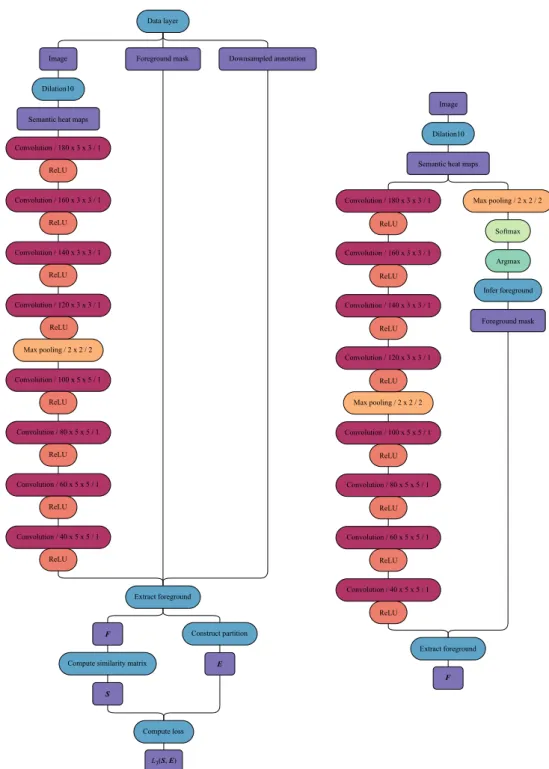
In our implementation, we removed the deconvolutional and softmax layers, and in-stead used the output of the context module as input to a third, “normalized cuts” module. Diagrams illustrating the conceptual structure of this module, during training as well as inference, are shown in Figure 4.2.

The data layer of the training network outputs three arrays: a preprocessed image, a downsampled version of the ground truth instance-level annotation of that image, and a binary foreground mask indicating which pixels of the downsampled annotation belong to the class we wish to partition. Image preprocessing consists merely of channel-wise mean subtraction, where the mean values were computed from the training data, as well as mirroring the image about its vertical axis with a probability of0.5. Downsampling of the ground truth annotation is done by means of majority vote among neighboring pixels.

The preprocessed image is passed through the front-end and context modules of the Dilation10 network, resulting in the19semantic heat maps mentioned earlier. Due to re-strictions in terms of hardware, as well as to speed up forward propagation, the heat maps of each image were computed in advance. Consequently, the data layer of our actual imple-mentation does not output a preprocessed image, but instead outputs the pre-computed heat maps and passes them directly to the normalized cuts module. What is more, the resolution of the Cityscapes images is too large for the Dilation10 network to handle, and to compute the128_⇥256pixel heat maps corresponding to a whole image required stitching together smaller heat maps computed from256_⇥512pixel image tiles. Hence, precomputing the heat maps was rather an attractive way to go.

The normalized cuts module contains a chain of eight convolutional layers. The pur-pose of these layers is to learn features that will result in similarity matrices suitable for object partitioning through normalized cuts. The number of convolutional layers and ker-nels to use, as well as the size of those kerker-nels, was determined primarily through experi-mentation. The number of kernels in the final convolutional layer was set to40to restrict the rank of the similarity matrix. To limit the size of the similarity matrix, a 2_⇥2 max pooling layer with a stride of2reduces the spatial extent of the feature maps to64⇥128 pixels. The final ReLU guarantees that each entry of the similarity matrix is non-negative.

The binary foreground mask output by the data layer is used to extract the pixels in the final feature maps and the downsampled ground truth annotation that correspond to the semantic class being subject to partitioning. The pixels extracted from the ground truth annotation are used to construct the target partition matrixE. Reshaping the tensor obtained by extracting the foreground pixels of the feature maps yields the feature matrix F, which in turn gives the similarity matrix through S = F FT. Finally, the loss layer evaluates L3(S,E) as given by (3.14). Forward propagation is identical during training

(39)

Figure 4.2:Networks used for training and validation (left), and for inference (right). The numerical codes that are associated with the convolutional layers and the pooling layers should be decoded as number of kernels ⇥ kernel height ⇥ kernel width / stride and

pooling height ⇥ pooling width / stride, respectively. All convolutional layers except the final one have biases.