Linear methods for regression and classification with functional data
Gilbert SaportaChaire de Statistique Appliquée & CEDRIC Conservatoire National des Arts et Métiers
292 rue Saint Martin, case 441 75141 Paris cedex 03, France
G. Damiana Costanzo
Dipartimento di Economia e Statistica Università della Calabria
Via P. Bucci, Cubo 0C
87036 Arcavacata di Rende (CS) - Italy [email protected]
Cristian Preda
Département de Statistique-CERIM, Faculté de Médecine, Université de Lille 2,
1, Place de Verdun, 59045 Lille Cedex, France [email protected]
Functional data occurs when we observe curves or paths from a stochastic process Xt . If for each curve or path we have a single response variable Y, we have a regression problem when Y is numerical, a classification problem when Y is categorical. We assume here that all trajectories are observed continuously on a time interval [0;T] and that the variables Y (when numerical) and Xt have zero mean.
1. Regression with a functional predictor
The functional linear model considers a predictor which may be expressed as an integral sum:
0
ˆ T ( ) t
Y =
∫
X β t dtThe problem is not new and comes back to Fisher (1924) who used the expression “integral regression”. It is well known that this regression model yields to an ill-posed problem: the least squares criterion leads to the Wiener-Hopf equation which in general has not an unique solution.
(
)
0
( t ) T t s ( )
E X Y =
∫
E X X β s dsand the problem is even worse when we try to estimate the regression coefficient function ( )t
β with a finite number of observations.
Since the works of Ramsay & Silverman (1997), many techniques have been applied to solve these kind of problem, mostly by using explicit regularization techniques. High dimensionality and multicollinearity also involves some smoothing. In the functional linear approach, functional data (the predictor) and functional parameter can be modelled as linear combinations of a basis functions from a given functional family. Literature on that subject essentially differs in the choice of the basis and the way parameters are estimated. Basis functions should be chosen to reflect the characteristics of the data: for example, Fourier basis are usually used to model periodic data, while B-spline basis functions are chosen as they have the advantage of finite support. We will focus here on linear methods based on an orthogonal decomposition of the predictors.
1.1 Linear regression on principal components (Preda & Saporta, 2005a)
The use of components derived from the Karhunen-Loeve expansion is, for functional data, the equivalent of principal components regression (PCR). The principal component analysis (PCA) of the stochastic process (Xt ) consists in representing Xt as:
1 ( ) t i i i X f t ξ ∞ = =
∑
where the principal components
0 ( )
T
i f t X dti t
ξ =
∫
are obtained through the eigenfunctions of the covariance operator:0 ( , ) ( ) ( )
T
i i
C t s f s ds=λ f t
∫
i .In practice we need to choose an approximation of order q :
1 cov( ; ) ˆ q i q i i i Y Y ξ ξ λ = =
∑
.But the use of principal components for prediction is heuristic because they are computed independently of the response: the components corresponding to the q largest
eigenvalues are not necessarily the q most predictive, but it is difficult to rank an infinite
number of components according to R2...
1.2 Functional PLS regression
PLS regression offers a good alternative to the PCR method by replacing the least squares criterion with that of maximal covariance between (Xt ) and Y .
2 0
max cov ( ,w Y w t X dt( ) t )
∞
∫
with w2 =1 The first PLS component is given by 1 .0 ( ) t
t =
∫
∞w t X dtdt ˆ
The PLS regression is iterative and further PLS components are obtained by maximizing the covariance criterion between the residuals of both Y and (Xt) with the previous components. The PLS approximation is given by:
( ) 1 1 0 ˆ ( )
ˆ ... ( )T
PLS q q q PLS q t
Y =c t + +c t =
∫
β t Xand for functional data the same property than in finite dimension holds: “PLS fits closer than
PCR” 2 2
( ) ( )
ˆ
( ; PLS q ) ( ; PCR q )
R Y Y ≥R Y Y since PCR components are obtained irrespective of the
response. In Preda & Saporta (2002) we show the convergence of the PLS approximation to the approximation given by the classical linear regression: limq→∞E Y( ˆPLS q( )−Yˆ 2) 0=
In practice, the number of PLS components used for regression is determined by crossvalidation.
2. Clusterwise PLS regression
Clusterwise regression may be used when heterogeneity in the data is present. This corresponds to a mixture of several regression models, that is, there exists latent categorical variable G with k categories defining the clusters such that:
0 2 ( / , ) ( ) ( / , ) g T t g E Y X G g X t dt V Y X G g α β σ = = = + = = =
∫
k is supposed to be known, but not the clusters.
Let us remind of the classical case for a finite number of predictors : for n observations, the cluster linear algorithm finds an optimal partition of the n points, and the
regression models for each cluster (element of partition) which minimize the criterion:
(
')
2 ˆ ( ) i g g i g i y − α +β x∑∑
The minimization is achieved by an alternated least squares algortihm of the k-means family alternating an OLS for each group (supposed known) and an allocation of each unit to the closest regression surface ie the model where the residual is minimal. Under the hypothesis that residuals within each cluster are independent and normally distributed, this criterion is equivalent to maximization of the likelihood function (Hennig, 2000).
For functional regression the previous model is not adequate and we have proposed to estimate the local models in each cluster by PLS regression in order to overcome this problem. The convergence of this algorithm has been discussed in (Preda & Saporta, 2005b) and clusterwise PLS functional regression has been applied to predict the behavior of shares of the Paris stock market on a certain lapse of time.
3. Binary classification with a functional predictor 3.1 Fisher’s linear discriminant analysis
Previous methods are easily generalized to binary classification, since Fisher’s linear discriminant function is equivalent to a multiple regression where the response variable Y is coded with 2 values a and b : most frequently ±1, but also conveniently 1 0
0 1
and - p p
p p with
(p0, p1) the probability distribution of Y.
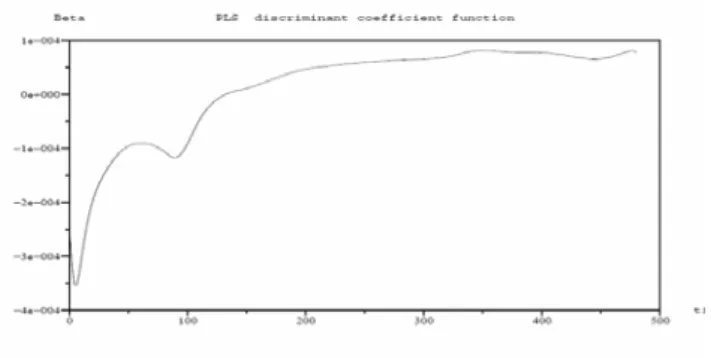
Costanzo D. et al. (2006) and Preda C. et al. (2007) have applied PLS functional classification to predict the quality of cookies from curves representing the resistance (density) of dough observed during the kneading process. For a given flour, the resistance of dough is recorded during the first 480 s of the kneading process. We have 115 curves which can be considered as sample paths of a L2-continuous stochastic process. Each curve is observed in 240 equispaced time points of the interval time [0, 480]. After kneading, the dough is processed to obtain cookies. For each flour we have the quality Y of cookies which can be Good, Adjustable and Bad. Our sample contains 50 observations for Y = Good, 25 for Y = Adjustable and 40 for Y = Bad . Due to measuring errors, each curve is smoothed using cubic B-spline functions with 16 knots.
Some of these flours could be adjusted to become Good. Therefore, we have considered the set of Adjustable flours as the test sample and predict for each one the group membership, Y = {Good, Bad}, using the discriminant coefficient function (Fig. 2) given by the PLS approach on the 90 flours. PLS functional discriminant analysis gave an average error rate of 11% which is better than discrimination based on principal components.
3.2 Functional logistic regression
Let Y be a binary random variable and the corresponding random sample associated to the sample paths ,
n y y1 ,… , ) (t xi i=1 ,… ,n.
A natural extension of the logistic regression (Ramsay et al., 1997) is to define the functional logistic regression model by :
0 ln ( ) ( )d ; 1, , 1 T i i i x t t t i π α β π ⎛ ⎞ = + = ⎜ − ⎟ ⎝ ⎠
∫
… n where πi =P(Y =1|X =xi(t);t∈T).It may be assumed (Ramsay et al., 1997) that the parameter function and the sample paths xi(t)are in the same finite space:
ψ ψ β =
∑
=b′ = p q q q t b t 1 ) ( ) ( ψ ψ i p q q iq i t c t x =∑
=c′ =1 ) ( ) (where ψ1(t),… ,ψq(t)are the elements of a basis of the finite dimensional space. Such an approximation transform the functional model (1) in a similar form to standard multiple logistic regression model whose design matrix is the matrix which contains the coefficients of the expansion of sample paths in terms of the basis, C=(ciq), multiplied by the matrix
, whose elements are the inner product of the basis functions ) d ) ( ) ( ( =
∫
= Φ T q k kq ψ tψ t t φ ln 1 π α π ⎛ ⎞ = + Φ ⎜ − ⎟ ⎝ ⎠ 1 C bwith b=(b1,…,bp), π =(π1,…πp)and 1being the p-dimensional unity vector.
Finally, in order to estimate the parameters a further approximation by truncating the basis expansion could be considered. Alternatively, regularization or smoothing may be get by some roughness penalties approach.
In a similar way as we defined earlier functional PCR, Leng and Müller (2006) use functional logistic regression based on functional principal components with the aim of classifying gene expression curves into known gene groups.With the explicit aim to avoid multicollinarity and reduce dimensionality, Escabias et al. (2004) and Aguilera et al. (2006) propose an estimation procedure of functional logistic regression, based on taking as covariates a reduced set of functional principal components of the predictor sample curves, whose approximation is get in a finite space of no necessarily orthonormal functions. Two different forms of functional principal components analysis are then considered, and two
different criterion for including the covariates in the model are also considered. Müller and Stadtmüller (2005) consider a functional quasi likelihood and an approximation of the predictor process with a truncated Karhunen-Loeve expansion. The latter also developed asymptotic distribution theory using functional principal scores.
Comparisons with functional LDA are in progress, but it is likely that the differences will be small.
3.3 Anticipated prediction
In many real time applications like industrial process, it is of the highest interest to make anticipated predictions. Let denote dt the approximation for a discriminant score considered on the interval time [0, t], with t < T. For functional PLS or logistic regression the score is but any method leading to an estimation of the posterior probability of belonging to one group gives a score. The objective here is to find t* < T such that the discriminant function d
0 ˆ( )
t
t t
d =
∫
X β t dtt* performs quite as well as dT .
For a binary target Y, the ROC curve and the AUC (Area Under Curve) are generally accepted as efficient measures of the discriminating power of a discriminant score. Let dt (x) be the score value for some unit x. Given a threshold r, x is classified into Y = 1 if dt (x) > r. The true positive rate or ”sensitivity” is P(dt > r|Y = 1) and the false positive rate or 1−”specificity”, P(dt > r|Y = 0). The ROC curve gives the true positive rate as a function of the false positive rate and is invariant under any monotonic increasing transformation of the score. In the case of an inefficient score, both conditional distributions of dt given Y = 1 and Y= 0 are identical and the ROC curve is the diagonal line. In case of perfect discrimination, the ROC curve is confounded with the edges of the unit square.
The Area Under ROC Curve, is then a global measure of discrimination. It can be easily proved that AUC(t)= P(X1 > X0), where X1 is a random variable distributed as dt whenY= 1 and X0 is independently distributed as dt for Y = 0. Taking all pairs of observations, one in each group, AUC(t) is thus estimated by the percentage of concordant pairs (Wilcoxon-Mann-Whitney statistic).
A solution is to define t* as the first value of s where AUC(s) is not significantly different from AUC(T) Since AUC(s) and AUC(T) are two dependent random variables, we use a bootstrap test for comparing areas under ROC curves: we resample M times the data, according to a stratified scheme in order to keep invariant the number of observations of each group. Let AUCm(s) and AUCm(T) be the resampled values of AUC for m = 1 to M, and δm their difference. Testing if AUC(s) = AUC(T) is performed by using a paired t-test, or a Wilcoxon paired test, on the M values δm.
The previous methodology has been applied to the kneading data: the sample of 90 flours is randomly divided into a learning sample of size 60 and a test sample of size 30. In the test sample the two classes have the same number of observations. The functional PLS discriminant analysis gives, with the whole interval [0, 480], an average of the test error rate of about 0.112, for an average AUC(T) = 0.746. The anticipated prediction procedure gives for M = 50 and sample size test n = 30 (same number of observation in each class), t* = 186. Thus, one can reduce the recording period of the resistance of dough to less than half of the current one.
4. Conclusion and perspectives
In this paper we addressed the problem of predicting a categorical or numerical variable Y with an infinite set of predictors Xt . We advocated linear models which are easy to
use and interpret; multicollinearity between predictors is best solved by PLS than by PCR. A clusterwise generalization is a way to take into account latent heterogeneity as well as some kind of non linearity.
For binary classification we proposed an anticipated prediction technique based on bootstrap comparisons of ROC curves.
Works in progress comprises the extension of clusterwise functional regression to binary classification, comparison with functional logistic regression as well as “on-line” forecasting: instead of using the same anticipated decision time t* for all data, we will try to adapt t* to each new trajectory given its incoming measurements.
References
Aguilera A.M., Escabias, M. & Valderrama M.J. (2006) Using principal components for estimating logistic regression with high-dimensional multicollinear data, Computational Statistics & Data Analysis, 50, 1905-1924
Costanzo D., Preda C. & Saporta G. (2006) Anticipated prediction in discriminant analysis on functional data for binary response. In COMPSTAT2006, 821-828, Physica-Verlag
Escabias, M., Aguilera A.M. & Valderrama M.J. (2004) Principal Component Estimation of Functional Logistic Regression: discussion of two different approaches. Nonparametric Statistics 16, 365-384.
Fisher R.A. (1924) The Influence of Rainfall on the Yield of Wheat at Rothamsted. Philosophical Transactions of the Royal Society, B: 213: 89-142
Hennig, C., (2000). Identifiability of models for clusterwise linear regression. J. Classification 17, 273–296.
Leng X. & Müller, H.G. (2006) Classification using functional data analysis for temporal gene expression data. Bioinformatics 22, 68-76.
Müller, H.G. & Stadtmüller, U. (2005) Generalized functional linear models. The Annals of Statistics 33, 774-805.
Preda C. & Saporta G. (2005a) PLS regression on a stochastic process. Computational Statistics and Data Analysis, 48, 149-158.
Preda C. & Saporta G. (2005b) Clusterwise PLS regression on a stochastic process. Computational Statistics and Data Analysis, 49, 99-108
Preda C., Saporta G. & Lévéder C., (2007) PLS classification of functional data, Computational Statistics