EFFICIENT SYNCHRONIZATION FOR GPGPU
by
Jiwei Liu
B.S., Zhejiang University, 2010
Submitted to the Graduate Faculty of
the Swanson School of Engineering in partial fulfillment
of the requirements for the degree of
Ph.D. in Electrical Engineering
University of Pittsburgh
2018
UNIVERSITY OF PITTSBURGH SWANSON SCHOOL OF ENGINEERING
This dissertation was presented by
Jiwei Liu
It was defended on June 12, 2018 and approved by
Jun Yang, Ph.D., Professor, Department of Electrical and Computer Engineering Rami Melhem, Ph.D., Professor, Department of Computer Science
Youtao Zhang, Ph.D., Associate Professor, Department of Computer Science Kartik Mohanram, Ph.D., Associate Professor, Department of Electrical and Computer
Engineering
Heng Huang, Ph.D., Professor, Department of Electrical and Computer Engineering Wei Gao, Ph.D., Associate Professor, Department of Electrical and Computer Engineering Dissertation Director: Jun Yang, Ph.D., Professor, Department of Electrical and Computer
EFFICIENT SYNCHRONIZATION FOR GPGPU
Jiwei Liu, PhD
University of Pittsburgh, 2018
High-performance General Purpose Graphics processing units (GPGPUs) have exposed bot-tlenecks in synchronizations of threads and cores. The massively parallel computing cores and complex hierarchies of threads present new challenges for synchronizations at different granularities. Performance of GPU is hindered by inefficient global and local synchroniza-tions. I propose hardware-software cooperative frameworks for efficient synchronization of GPGPU to address the following issues.
To provide efficient global synchronization (Gsync), an API with direct hardware support is proposed. The GPU cores are synchronized by an on-chip Gsync controller. Partial context switch is employed to guarantee deadlock-free execution. The proposed Gsync avoids expensive API calls and alleviates data thrashing. Prioritized warp scheduling is used to increase the overlap of context switch with kernel execution.
To efficiently exploit the inherent parallelism of producer-consumer problems, a flexible wait-signal scheme is proposed at thread-block level. I propose dedicated APIs to express fine-grained static and dynamic dependencies with hardware support. The proposed scheme can accelerate wavefront, graph and machine learning applications. The architectural de-sign of on-chip wait-de-signal controller eliminates busy wait loop and long-latency memory operations. I also propose thread block dispatch scheduling to address the problem of load imbalance and large context switch overhead.
To reduce stall due to synchronizations, a synchronization-aware warp scheduling is pro-posed to coordinate multiple warp schedulers upon synchronization events. Both perfor-mance and hardware utilization are improved by resolving the barrier sooner.
TABLE OF CONTENTS
1.0 INTRODUCTION . . . 1
1.1 THE CHALLENGES FOR GPGPU SYNCHRONIZATION . . . 4
1.1.1 Inefficient Global Synchronization . . . 4
1.1.2 Lack of Wait-Signal Support . . . 4
1.1.3 Synchronization Oblivious Warp Scheduling . . . 5
1.2 THESIS OVERVIEW . . . 6
1.3 CONTRIBUTIONS . . . 9
1.3.1 Efficient GPU Global Synchronization with Light Weight Context Switch 9 1.3.2 Accelerate RNNs with software Wait-Signal . . . 9
1.3.3 Thread Block Level Wait and Signal in GPU with Hardware support . 10 1.3.4 Synchronization Aware GPGPU Warp Scheduling . . . 11
1.4 THESIS ORGANIZATION . . . 12
2.0 BASICS OF GPGPU . . . 13
2.1 GPGPU ARCHITECTURE . . . 13
2.2 STREAMING MULTIPROCESSOR ARCHITECTURE . . . 13
2.3 WARP SCHEDULING . . . 14
2.4 GPU SYNCHRONIZATION PRIMITIVES . . . 15
2.4.1 Global Synchronization . . . 15
2.4.2 Within-TB synchronization . . . 15
3.0 RELATED WORKS . . . 21
3.1 ADDRESSING GLOBAL SYNCHRONIZATION . . . 21
3.1.2 Atomic Operations and Memory Flags . . . 22
3.1.3 Persistent threads . . . 22
3.1.4 Cooperative Kernels . . . 23
3.1.5 Occupancy Discovery Protocol . . . 23
3.2 ADDRESSING PRODUCER CONSUMER PROBLEMS . . . 24
3.2.1 Asynchronous Task Management Interface . . . 25
3.2.2 Specialized Warps . . . 25
3.2.3 Case Study: RNN Acceleration Techniques . . . 26
3.2.3.1 Accelerating Single Layer RNNs . . . 29
3.2.3.2 Accelerating Multi-Layer RNNs . . . 30
3.2.3.3 Stream implementations of RNNs . . . 30
3.2.3.4 Persistent implementations of RNNs . . . 34
3.3 ADDRESSING WARP SCHEDULING. . . 34
3.3.1 Round Robin Warp Scheduling . . . 34
3.3.2 Greedy Then Oldest Warp Scheduling . . . 35
3.3.3 CTA-aware two-level warp scheduling . . . 35
4.0 EFFICIENT GLOBAL SYNCHRONIZATION . . . 36
4.1 MOTIVATIONS FOR EFFICIENT GSYNC . . . 36
4.2 GPU-SIDE GLOBAL SYNCHRONIZATION API . . . 38
4.3 MICROARCHITECTURE DESIGN FOR GSYNC . . . 40
4.4 MANAGING CONTEXT SWITCH . . . 43
4.4.1 Memory Allocation for Context Saving . . . 43
4.4.2 Reducing Context Switch Overhead. . . 44
4.4.3 Reducing Memory Congestion . . . 46
4.4.4 Using Other Context Switch Techniques . . . 46
4.5 Experimental Results for Global Synchronization . . . 47
4.5.1 Experiment Setup and Methodology . . . 47
4.5.1.1 Stencil applications . . . 50
4.5.1.2 Graph Traversal. . . 51
4.5.3 Hardware Overhead Analysis . . . 54
5.0 ACCELERATING RNN WITH SOFTWARE WAIT-SIGNAL . . . 55
5.1 ALGORITHM . . . 55
5.1.1 Fine-grained Parallelism within a layer . . . 56
5.1.2 Implementing Wait Signal with memory flags . . . 58
5.1.3 Workload Assignment . . . 59
5.2 Experimental Results for evaluation RNN . . . 61
5.2.1 Benchmarks . . . 64
5.2.2 Speedup Comparison . . . 65
6.0 THREAD-BLOCK LEVEL WAIT SIGNAL WITH HARDWARE SUP-PORT . . . 69
6.1 SYNTAX AND USAGE OF WAIT AND SIGNAL IN GPU . . . 69
6.1.1 Developing Usage for Static Dependencies . . . 70
6.1.2 Developing Usage for Dynamic Dependencies . . . 74
6.2 COMBINING KERNELS TO AVOID GLOBAL SYNCHRONIZATION . . 75
6.3 ARCHITECTURE DESIGN . . . 76
6.3.1 Virtualizing Event Counters . . . 77
6.3.2 Integration with Partial Context Switching . . . 78
6.3.3 Specifying the order of TB Dispatching . . . 80
6.4 Experimental Results of the proposed Wait-Signal Scheme . . . 82
6.4.1 Experimental Methodology . . . 82
6.4.2 Results for Graph Applications . . . 82
6.4.3 Results for Wavefront Applications. . . 83
6.4.4 Overhead Analysis . . . 85
7.0 SYNCHRONIZATION AWARE GPGPU WARP SCHEDULING . . . 93
7.1 KEY OBSERVATIONS OF SAWS . . . 94
7.1.1 The Anatomy of Synchronization Events . . . 95
7.1.2 Reducing Intra-CTA Interference . . . 96
7.1.3 Removing Barriers at the Same Rate . . . 97
7.3 INTEGRATING WITH PRIOR WARP SCHEDULER . . . 99
7.4 Warp Scheduling Experimental Results . . . 100
7.4.1 Performance Improvement, SAWS vs. GTO and CATLS. . . 101
7.4.2 SAWS Reduces Barrier Waiting Time . . . 101
7.4.3 SAWS Ensures Uniform Barrier Clearing Rate among CTAs . . . 102
8.0 FUTURE RESEARCH DIRECTIONS . . . 104
8.1 SINGLE-NODE MULTI-GPU SYNCHRONIZATION . . . 105
8.2 Multi-NODE MULTI-GPU SYNCHRONIZATION . . . 107
9.0 CONCLUSION . . . 108
LIST OF TABLES
1 Overview of proposed schemes and challenges . . . 7 2 Configurations of GPGPU-Sim for evaluation of global synchronization. . . . 48 3 Configurations of GPU devices for RNN speedup comparison . . . 63 4 Communication for multiple GPUs. P2P: peer-to-peer GPU communication. [1]104
LIST OF FIGURES
1 Thread hierarchy of GPU programs . . . 2
2 General GPGPU architecture. SM: Streaming Multiprocessor . . . 3
3 Problem overview: (a) global synchronization (b) wait-signal support (c) Syn-chronization oblivious scheduling . . . 7
4 GP100 Pascal GPU architecture [2]. . . 17
5 Architecture of Streaming Multiprocessor. . . 18
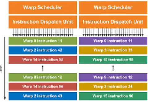
6 Warp scheduling: warps from the same TB are split. . . 19
7 Host code examples of CPU driven synchronizations through repeated kernel launch. (a) stencil computation. (b) convolutional neural network. . . 19
8 Programming patterns with the within-TB synchronization. . . 20
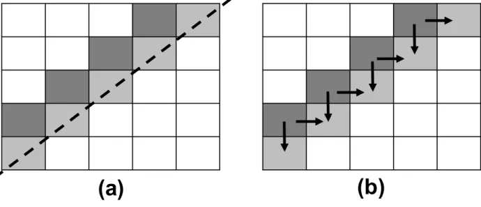
9 (a) barrier (wavefront) synchronization vs (b) wait-signal synchronization. Com-puting each tile only depends on the upper and left tiles. . . 24
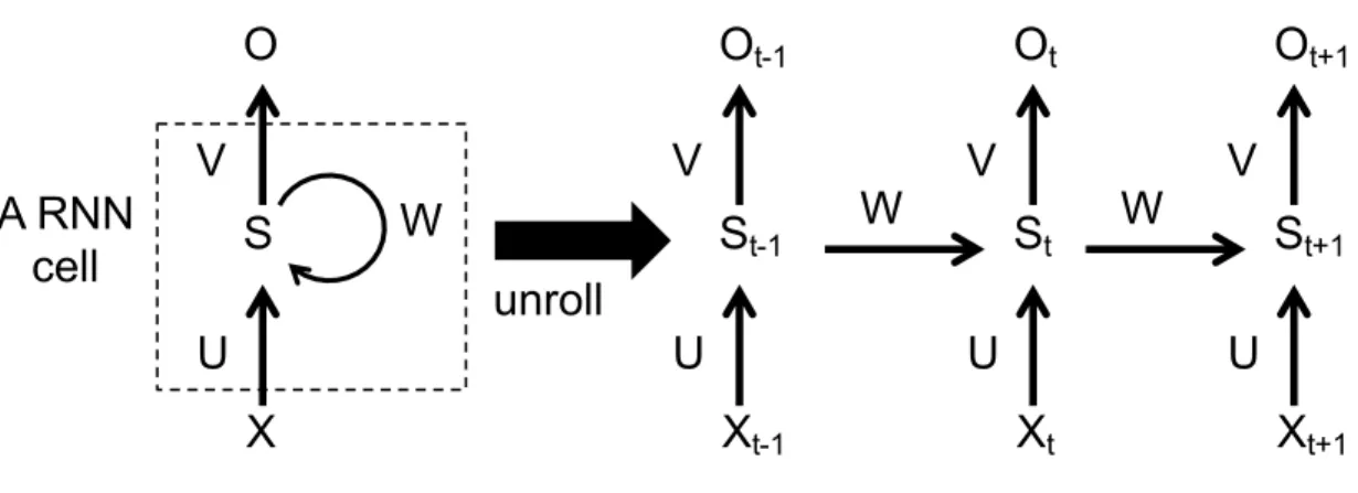
10 A basic single recurrent neural network cell. . . 27
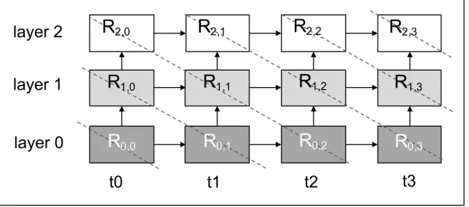
11 Multi-layer RNNs. The dashed line indicates potential wavefront parallelism. Ri,t represents a RNN cell at layer i and time step t. The RNN cells of the same layer (same shades) share the same weights.. . . 31
12 Stream Implementation of wavefront parallelism. W: wait event. S: signal event. Ri,t represents akernelto compute a RNN cell at layeriand time step t. 32 13 Percentage of reused weights in RNNs with batch size = 4 . . . 32
14 Persistent RNN. The dashed line indicates global barrier. Each Ri,t is com-puted by all TBs sequentially. . . 33
16 Global synchronization through (a) CPU-side API and repeated kernel launch-ing: (1) kernel execution, (2) data flushing, (3) kernel launch overhead, (4) data
reload; (b) the proposed GPU-side synchronization. . . 37
17 (a) Percentage of reused data across global barrier. (b) ideal speedup over repeated kernel launching if there is no data thrashing.. . . 38
18 Code examples of using globalSync(): (a) stencil computation; (b) CNN application. . . 39
19 Architecture support for Global Synchronization with Partial Context Switch and meta data for swapped-out TBs. . . 41
20 Breakdown of context size reduction. . . 45
21 Scheduling swap instructions when TB0 & TB1 are swapped out and TB2 & TB3 are swapped in (to/from global memory). (a) Baseline. (b) Proposed.. . 47
22 API call latency for different data size and applications. . . 49
23 Correlation between simulated and real device execution on GTX 970. . . 49
24 Speedup for stencil 2D. . . 50
25 Speedup for BFS. . . 53
26 Performance overhead of partial context switch normalized to an ideal GS.. . 54
27 The proposed TB-level wait-signal. The light/dark blue arrays are write/read memory flag arrays. The entire network is computed by one kernel and for eachi, the cells Ri,t, t= 0,1, ...are computed by a subset of TBs. . . 56
28 Fine-grained Parallelism within an RNN cell. Si,t−1W and Oi−1,tU run in parallel by different threads. . . 57
29 Memory flag arrays to implement TB-level wait-signal. (a) Each TB reads its own entry in the read memory flag array. (b) All TBs read the same entry in the read memory flag array . . . 60
30 Comparing the TB layout of persistent RNN (W-prnn) and the proposed wait-signal mechanism (W-ws).. . . 62
31 The layout of TB dimensions of the proposed scheme. The TB’s width is multiples of 32 threads (32s). . . 63
33 Speedup comparison for GRU RNN. . . 67
34 Speedup comparison for LSTM RNN. . . 67
35 (a) Summed area table (SAT) with static one-to-many and many-to-one de-pendencies. (b) SAT using PT produces one-to-one dede-pendencies. . . 71
36 The use of local synchronization in one-pass SAT. . . 72
37 (a) All pair shortest path (APSP) with static many-to-many dependencies. (b) Breadth first search (BFS) with dynamic dependencies (the number in each node indicates the TB that is processing that node). . . 86
38 The use of wait and signal primitives to enforce dynamic dependenciesin the BFS algorithm.. . . 87
39 TB dependencies in the LUD application. . . 87
40 Skeleton of LUD (a) Global synchronization through repeated kernel launch. (b) wait-signal using a combined kernel . . . 88
41 Microarchitecture support for Wait and Signal . . . 88
42 Integration with context switch engines. . . 89
43 Comparing graph applications with sampled data sets (40k nodes). . . 89
44 Comparing graph applications with the original data sets (1M nodes). . . 90
45 Comparing SAT with varied data size. . . 90
46 Comparing SOR with varied data size. . . 91
47 Comparing LUD with varied data size.. . . 91
48 Measuring the effect of event grouping and counter virtualization using the LUD application. . . 92
49 Performance of single vs. twoscheduler SMs for synchronization-rich kernels. . 94
50 Performance of single vs. twoscheduler SMs for synchronization-free kernels. . 95
51 Timing of synchronization events . . . 96
52 CTA promotion could cause nonuniform barrier-clearing rate. . . 97
53 Performance comparisons for synchronization-rich benchmarks. . . 100
54 Breakdown of barrier waiting time. . . 102
56 Single node Multiple GPU global synchronization via memory flags enabled by unified virtual memory and demand paging. Dashed arrow: read and write. Solid arrow: write. . . 106
1.0 INTRODUCTION
Graphics Processing Units (GPUs) were originally designed to accelerate computer graphics and vision related tasks such as texture mapping [3], ray tracing [4], vertex shading [5] and etc, which are commonly used in video games and 3D rendering [6]. Dating back to 1995, the first GPU was introduced as a 3D graphics add-in chip [7]. During the early 2000s, the major goal of GPU design is how to deliver more polygons with high frame rates to increase the realism of 3D rendering [6]. The nature of geometric and graphics computation is highly parallel and heavily floating-point intensive. The raw throughput requirement of such operations impose a vast pressure on the traditional general-purpose CPU processors. Inspired by the good performance of GPU, scientific researchers and software developers started looking for ways to apply GPUs beyond computer graphics to more general purpose computing.
Programming GPUs used to be notoriously difficult for any simple tasks other than graphics applications [6]. Programmers have to be aware of the low-level hardware details such as the fixed graphics pipelines. Programming languages and interfaces were also limited to graphics-centered APIs such as OpenGL [8], DirectX [9], C for Graphics (CG) [10].
Numerous efforts have been made in the research and industry community to improve GPU programmability. The most successful projects include Compute Unified Device Ar-chitecture (CUDA) [11] form NVIDIA and Open Computing Language (OpenCL) [12]. Both CUDA and OpenCL are general-purpose programming models for parallel computing. CUDA is vendor-specific model which is available only to NVIDIA GPUs and accelerators while OpenCL is an open cross-platform standard for all vendors which supports not only GPUs but also CPUs, digital signal processors (DSPs), field-programmable gate arrays (FP-GAs) and other hardware accelerators [12, 13]. CUDA and OpenCL support C as well as
other high level programming languages. With widely uptake of CUDA and OpenCL within the academic and industry community, GPU is turned from graphics-centric platform into general-purpose usage, hence the term general-purpose GPU (GPGPU) computing.
Nowadays GPGPU is becoming increasingly popular for a wider range of applications including machine learning, data mining, computational biology and many more scientific and commercial applications. Deep learning and deep neural networks (DNNs) have re-cently gained attention due to their superior performance and ground-breaking results in various application domains such as computer vision [14], speech recognition [15], and nat-ural language processing [16]. GPGPU is the most successful hardware to accelerate DNN applications [14,17,18,19], including both training and inference, thanks to its tremendous compute horsepower and highly optimized software libraries such as cuDNN [17], tensorflow [20], caffe [21] and so on.
warp
kernel Thread block
thread
Figure 1: Thread hierarchy of GPU programs
A typical GPU program consists of multiple kernels of thousands of threads. The thread hierarchy is shown in Figure 1. These threads are organized in thread blocks, or TB in short [11, 22] (also known as work groups [23]). A kernel is simply a grid of TBs. Within a TB, a group of threads that are executed in lockstep and scheduled as a unit is referred to as a warp or a wavefront. A warp consists of 32 threads on NVIDIA hardware [11] and a wavefront consists of 64 threads in AMD hardware [23]. As shown in Figure 2, a GPU consists of Streaming Multiprocessors (SM) (also known as Compute Units) with their own shared memories and L1 data caches. Each SM has one or more independent warp schedulers that can quickly switch contexts between threads and issue instructions from different ready
warps. To initialize a kernel, the TB dispatcher dispatches TBs to SMs until all SMs reach their maximum capacities [22]. Then the warp scheduler within a SM picks a ready warp to execute in each cycle. The warp is selected based on a warp scheduling policy such as the round robin policy (RR).
SM
SM
SM
SM
Interconnection Network
L2 cache
Memory
controller
L2 cache
Memory
controller
L2 cache
Memory
controller
GPGPU
Figure 2: General GPGPU architecture. SM: Streaming Multiprocessor
In efficient parallel algorithms, threads cooperate and share data to perform collective computations. To share data, the threads must synchronize. The granularity of sharing varies from algorithm to algorithm, so thread synchronization should be flexible. Histori-cally, programming models for GPU, including CUDA and OpenCL, have provided a single and simple construct for synchronizing cooperating threads: a barrier across all threads of a thread block, as implemented with the syncthreads or barrier function. Such barrier synchronization is a point in a program where a thread may not proceed further until other parallel threads, in this case threads from the same TB, reach this point. On the other hand, synchronization of TBs or threads from different TBs are not allowed within the kernel. The only operation to achieve such synchronization is to terminate the current kernel and launch the kernel again. All threads of the kernel are synchronized at the kernel boundary hence a global synchronization of all threads are realized. This shows a fundamental design philos-ophy of current GPU synchronization. By not allowing threads in different TBs to perform barrier synchronization with each other, GPU run-time system does not need to deal with
any constraint while executing different TBs. In other words, TBs can execute in any order relative to each other since none of them need to wait for each other. This flexibility enables transparent scalability [11,22]. Without changing the code, the performance of the program scales naturally with different hardware configurations (different number of cores).
However, programmers often need to define and synchronize groups of threads larger or smaller than thread blocks in order to enable greater performance, design flexibility, and exploit finer parallelism. Therefore hardware and architectural modifications are necessary for efficient, flexible and reliable synchronization mechanisms.
1.1 THE CHALLENGES FOR GPGPU SYNCHRONIZATION
1.1.1 Inefficient Global Synchronization
Current GPU global synchronization (Gsync) across the entire grid of threads is inefficient. Gsync is typically achieved by slicing a kernel at the synchronization points, often leading to repeated kernel launches [11, 12]. Such an approach incurs overhead due to API calls and data thrashing. Previously, these overhead are deemed acceptable since many parallel processing have long-latency kernels which outweighs those overheads. However, with the recent development of real-time deep learning applications such as image recognition in self-driving cars [24] and speech recognition [15] in instantaneous speech to text (STT), the response time of inferring one image or one sentence (not training) is crucial. In those scenarios, each kernel finishes in several hundreds of microseconds, which makes kernel launch Gsync-related overhead more pronounced. Existing software workarounds such as atomic operations and memory flags may lead to deadlock when the GPU cannot simultaneously host all the threads [25].
1.1.2 Lack of Wait-Signal Support
GPU performance on applications with irregular parallelism and producer-consumer depen-dencies has suffered from a limited support for synchronization primitives. For these
prob-lems, global synchronization unnecessarily involves all the thread blocks. Existing software partial synchronization across thread blocks use atomic operations or memory flag-arrays, which rely on busy-wait loops that can cause underutilization of hardware resources and may lead to deadlock for large data sizes [26]. Specialized Warps [27] present a hardware solution that achieves partial synchronization among the warps of a thread block but do not extend to synchronization between thread blocks. Cooperative groups [28] can also synchronize thread blocks but are not flexible and efficient enough to express fine-grained dependencies. Hetero-geneous system architecture (HSA) and Asynchronous Task Management Interface (ATMI) [13, 29] implement wait-signal at kernel level with dedicated APIs and task queues, which is less effective utilizing GPU hardwares compared to thread block (TB) level wait-signal schemes. Dynamic parallelism [11, 13] is also a kernel-level optimization for data depen-dent workloads but is not efficient for applications with static dependencies due to excessive launching of children kernels for small tasks.
One classic application to demonstrate the importance of wait-signal mechanism is Re-current neural network (RNN). RNNs are an important family of deep learning models which can learn the sequential pattern of input data. Multi-layer RNNs have two unique properties: 1) wavefront parallelism across layers and time steps and 2) reusing weights over multiple time steps during inference. Previous GPU-accelerated RNNs exploit these two optimiza-tion opportunities separately. Specifically, the wavefront synchronizaoptimiza-tion is realized with kernel-level APIs such as hsa signal wait acquireor cudaStreamSynchronize. Preserving the weights using on-chip registers are achieved by persistent thread models at the thread block level which rely on global synchronization barriers to enforce the dependencies.
1.1.3 Synchronization Oblivious Warp Scheduling
Traditional warp scheduling policies of GPGPU have been optimized to increase memory latency hiding capability [30], improve cache behavior [31], and alleviate branch divergence [32]. However, warp scheduling policies do not account for the synchronization behavior among warps under the presence of multiple warp schedulers. A warp may stall the cores due to a thread incurring a long latency operation. Hence, GPGPU SMs can switch to
different warps to continue execution and stay active. On every cycle, a scheduler makes the decision on which warp to issue next. An uninformed execution order of warps may create unnecessary scheduling stalls and SM idle times. Barrier synchronizations, which are used to coordinate execution among threads, are adopted in a wide range of general purpose applications. The most common barrier is the TB-level barrier, where all threads of a TB have to arrive at a single point before any of them can proceed. A TB is assigned entirely to one SM. I made a key observation that the warps within a TB are distributed evenly to each scheduler of an SM to balance the load. Hence, each scheduler only sees part of one TB, and performs scheduling independently of other schedulers. Their scheduling decisions and order are also entirely different. When synchronization barriers are present, hitting the same barrier on different schedulers could be very far apart in time, causing earlier warps to stall for a long time waiting for the latest warp to clear out the barrier. None of the existing warp schedulers address this issue due to their synchronization unawareness.
1.2 THESIS OVERVIEW
The problems to be solved are summarized in Figure 3. Figure 3(a) shows the global syn-chronization where all threads and TBs are synchronized at a global barrier. Since the number of TBs can exceed the capacity of GPU, synchronizing all TBs requires marking the status of each TB and context switch out and in TBs appropriately. Figure 3(b) shows the problem of implementing wait-signal scheme at TB level. Producers and consumers are placed in different TBs. Consumer TBs should be blocked until a signal is received from the producer TB it depends on (the red arrow in Figure 3(b)). Figure 3(c) shows the prob-lem of synchronization oblivious warp scheduling. The warps of the same TB are split and distributed to each warp scheduler. If a within-TB barrier is used in the kernel, the barrier will introduce additional delay since the two warp schedulers do not communicate with each other. To solve these problems, I propose several architectural techniques as summarized in Table 1 with the major challenges for each scheme. For global synchronization, I propose an efficient hardware support to synchronize thread blocks globally within the kernel. A
hardware counter is used to manage a global barrier across thread blocks and partial context switch is leveraged to avoid deadlock. Moreover, we design several techniques to reduce the context switch overhead which is critical to performance improvement. The proposed scheme outperforms repeated kernel launch when 1) data reuse is significant across synchronization points and/or 2) the latency of the API calls is relatively long.
kernel kernel kernel
Warp
scheduler 1 scheduler 2Warp
(a) (b) (c)
Global Barrier Signal
Figure 3: Problem overview: (a) global synchronization (b) wait-signal support (c) Synchro-nization oblivious scheduling
Table 1: Overview of proposed schemes and challenges
# Scheme Challenges
1 Global Synchronization Large contexts to save
2 TB-Level Wait-Signal Complex producer-consumer patterns 3 Synchronization-Aware Warp Scheduler No cooperation of warp schedulers
For wait-signal support, I propose a hardware-software cooperative framework to achieve Wait-Signal mechanism between thread blocks in GPGPUs to efficiently exploit the inherent parallelism of producer-consumer problems. The proposed scheme guarantees deadlock-free execution and improves load balancing. The global thread block dispatcher is augmented with a wait-signal controller to manage event counters and synchronization of thread blocks.
To avoid busy wait loops, the ”Wait” instruction blocks a TB and releases its computing resources for use by other TBs. The happen-before relationships of ”Signal” and ”Wait” is resolved by allowing both wait and signal instructions to increment an event counter while only wait instructions are blocking. The proposed wait-signal mechanism is flexible to support both static and dynamic producer consumer dependencies. In order to achieve load balancing and avoid unnecessary context switch, we propose a kernel configuration extension to initialize the order of TB dispatching based on the dependencies implied by the applications.
To accelerate RNNs as a representation of producer-consumer problems, we propose a novel wait-signal mechanism at the thread block (TB) level to accelerate multi-layer RNNs. The multi-layer RNN is launched in a single kernel where weights are loaded in registers only once and persist for all the unfolded time steps. The weights of each layer are statically allocated to a specific group of TBs that collaborate to accomplish one computing task for the current time step (namely matrix multiplication). After synchronizng using a local barrier, the TB group assigned to a given layer signals the TB groups assigned to the next layer and waits for the results from the previous layer before proceeding with the computation for the next time step. The local barrier and the wait signals are implemented by lock-free memory flags. With the proposed TB-level wait-signal mechanism, the wavefront parallelism is achieved and unnecessary memory reloading of weights is avoided. We implemented the proposed wait-signal mechanisms on the latest GPUs and evaluated the speedups using a number of widely used RNNs. On average, the proposed scheme achieves 37% speedup over the state-of-the-art persistent RNNs.
To improve performance of within-TB synchronization in the context of multiple warp schedulers, I propose a warp scheduling algorithm that is synchronization aware. The key observation is that excessive stall cycles may be introduced due to synchronizing warps residing in different warp schedulers. We propose that schedulers coordinate with each other to avoid warps from being blocked on a barrier for overly long. Such coordination will dynamically reorder the execution sequence of warps so that they are issued in proximity when a barrier is encountered.
1.3 CONTRIBUTIONS
1.3.1 Efficient GPU Global Synchronization with Light Weight Context Switch
I propose a new global synchronization (Gsync) function at the GPU-side, which applies to both conventional SPMD and persistent programming styles. The existing SM and TB dispatcher is augmented to manage GS and partial context switches of the TBs. I also pro-pose effective techniques for reducing the overhead of context switching to achieve scalabil-ity. The experimental results show that the proposed scheme outperforms existing software approaches in three typical type of applications with up to 2x speedup over CPU-driven synchronization. I make the following contributions.
• An extensive study on the effectiveness and trade-offs of the existing software approaches for Gsync in both CUDA and OpenCL
• efficient approach to explicitly support global synchronization using partial context switch to avoid deadlocks. The proposed approach improves both performance and programma-bility.
• Case studies of representative applications, including scientific computing, graph traver-sal and machine learning, to demonstrate how to use the proposed Gsync function call and benefit from its performance advantages.
1.3.2 Accelerate RNNs with software Wait-Signal
I propose a novel wait-signal mechanism at the thread block (TB) level to accelerate multi-layer RNNs. First, we implement thewait() andsignal() functionality via lock-free memory flags [25]. A TB that calls a wait() function will be stalled until its dependent TBs exe-cute a signal() function. With such fine-grained synchronization, the theoretical maximum wavefront parallelism can be achieved. The proposed scheme also improves the computation efficiency and the reuse of shared memory. Specifically, in the proposed scheme, the weights of a certain layer are partitioned among TBs, which is different from the state-of-the-art persistent RNN scheme[33], where the weights of the entire neural network are partitioned among TBs. I make the following contributions:
• A study of the potential for accelerating RNNs with both wavefront parallelisms and on-chip storage of weights.
• The design of an efficient wait-signal functionality at the TB-level using memory flags. This increases both parallelism and hardware occupancy for RNN implementations. • Experimentation with different representative RNN applications to demonstrate the
im-pact of key hyper parameters such as number of layers, feature dimensions and sequence length on the proposed design.
1.3.3 Thread Block Level Wait and Signal in GPU with Hardware support
I propose a Wait-Signal mechanism with hardware support for local synchronization of thread blocks in GPGPUs. Each Streaming Multiprocessor is augmented with wait and signal buffers and extend the global thread block dispatcher with a wait-signal controller to manage event counters. The proposed scheme can be integrated with context switch engines that were previously proposed for swapping TBs when all the TBs of a kernel cannot fit simultaneously on the GPU. I also propose a mechanism that allows applications to control the order of TB dispatching, thus eliminating the need for context switching in single pass wavefront application kernels as long as the TBs constituting an active front can fit on the GPU.
The proposed mechanism can support one-to-one, one-to-many, to-one, and many-to-many producer consumer dependencies. Cycle-accurate simulation shows that, on average, the proposed scheme achieves 2.0x speedup over repeated kernel launch and 31% speedup over the best-known software memory flags techniques. I make the following contributions.
• An extensive study of the effectiveness and trade-offs of the existing approaches for producer-consumer relationships.
• An efficient approach to explicitly support Wait and Signal in hardware to exploit fine-grained parallelism, guarantee deadlock-free execution and improve load balancing. • Case studies of representative applications executing wavefront and graph algorithms.
1.3.4 Synchronization Aware GPGPU Warp Scheduling
I propose Synchronization Aware GPGPU Warp Scheduling (SAWS) to tackle warp schedul-ing to mitigate performance loss due to synchronization events in SMs with multiple sched-ulers. Current designs treat each scheduler independently, which works well without syn-chronization barriers, but exposes deficiency with barriers. I find that multiple schedulers, when operating independently, will delay the clearance of barriers and create excessive stall cycles to the warps. Hence, I propose to coordinate among multiple schedulers and priori-tizes warps as a reaction to synchronization events. In addition, I find that maintaining a uniform barrier-clearing rate during prioritization brings additional performance benefit.
Our proposed scheme SAWS is so simple that integrating it with existing scheduler does not require much additional hardware. The evaluation shows that SAWS can speed up barrier clearance by 15% and total execution by 10% on average, when compared with the state-of-the-art warp scheduler. Finally, SAWS shows its increasing effectiveness when the number of scheduler grows, proving that it is a scalable design. Specifically I make the following contributions.
• A detailed analysis of performance loss due to mishandling of synchronization barriers with multiple warp schedulers.
• A simple synchronization aware warp scheduling algorithm that coordinates multiple schedulers to minimize barrier waiting time and synchronization-induced stalls.
• A design that can be seamlessly integrated with existing warp scheduler so that synchronization-rich kernels can be well handled while not harming synchronization-free kernels.
• A simulation evaluation of performance advantages of the proposed scheduler over exist-ing well-studied warp schedulers.
1.4 THESIS ORGANIZATION
The rest of this thesis is organized as follows. Chapter 2 presents preliminary information of GPGPU. Chapter 3 discusses the related work. The efficient global synchronization is described in Chapter 4. Software implementation of wait-signal to accelerate RNNs are introduced in Chapter 5. Chapter 6 illustrates the thread-block level wait-signal scheme. The synchronization-aware warp scheduling is explained in Chapter 7. Chapter 8 describes the future research directions. Chapter 9 concludes the thesis.
2.0 BASICS OF GPGPU
2.1 GPGPU ARCHITECTURE
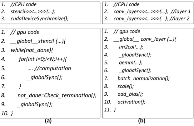
General Purpose Graphic Processing Units (GPGPUs) have been evolved actively in recent years with increasing number of cores, higher clock frequency and bandwidth high-capacity on-board GPU memory. For example, the state-of-the-art Nvidia Pascal GPU architecture is shown in Figure4[2]. The SMs are grouped into Texture Processing Clusters (TPCs) and Graphics Processing Clusters (GPCs). The global GigaThread controller man-ages TB dispatching, application context switching and also provides a pair of streaming data-transfer engines, each of which can fully saturate GPU’s PCI Express host interface.
Each memory controller is attached to 512 KB of L2 cache, and each High Bandwidth Memory (HBM) DRAM stack is controlled by a pair of memory controllers. The full GPU includes a total of 4096 KB of L2 cache. L1 cache can serve as a texture cache depending on workload. The unified L1/texture cache acts as a coalescing buffer for memory accesses, gathering up the data requested by the threads of a warp prior to delivery of that data to the warp.
2.2 STREAMING MULTIPROCESSOR ARCHITECTURE
The most critical component of GPU is the streaming multiprocessor, or SM in short. As shown in Figure 5, Each SM consists of many simple scaler processors (SP) for common simple calculations such as addition and several special function units (SFUs) for complex calculations such as exponential operations. There are abundant of registers on the SM
private to each thread. There is also a L1 data cache which can cache global memory access shared by all threads on the SM. Different from CPU, the capacity of registers (96 KB) on the SM is larger than that of the L1 cache (48 KB). The shared memory is a special scratch memory that is programmable and to be shared by threads from the same TB. In previous GPU architecture, shared memory and L1 cache are physically the same device and can be configured/split by programmers. Recent GPU architecture provides dedicated independent shared memory and L1 cache.
2.3 WARP SCHEDULING
As shown in Figure 5, there are multiple warp schedulers in one SM. The number of warp schedulers range from two to four.
When a kernel is dispatched to a GPGPU, a global TB dispatcher assigns TBs to SMs until all SMs are saturated. An SM may be assigned more than one TB at a time, since the size of a kernel and its TBs may vary. An SM which finishes a TB will get a new one from the global dispatcher, until all TBs of a kernel finish. Hence, the execution latency of a kernel is dependent on how quickly the SMs complete their TBs.
As the core count increases in the latest generations of GPGPUs, each SM may contain one, two or four warp schedulers. When a TB is assigned to an SM, its warps are further assigned to those warp schedulers in a round robin fashion in order to balance the warp distribution, as shown in Figure 30. During execution, each warp scheduler selects a ready warp to execute, allowing one, two or four warps to issue and execute concurrently. A warp can become blocked due to a long latency operation such as a load from the memory or a barrier synchronization. The warp scheduler switches context to another ready warp, if such warp can be found, to mask the stalled cycles due to long latency operations. If no such warps can be found, the scheduler stalls, causing resource underutilization. In fact, how the warps are selected to execute determines the resulting number of stalled cycles. Hence, effort has been put on optimizing the scheduler to mask or reduce stall cycles.
2.4 GPU SYNCHRONIZATION PRIMITIVES
2.4.1 Global Synchronization
Figure7shows host (CPU) code examples where kernels are sequentialized by either implicit or explicit CPU-driven synchronizations. As such programming style typically puts kernels and synchronizations in loop bodies, we term this synchronization method “repeated kernel launching”. In Figure7(a), the kernel stencil is invokedN times (line 3) within the inner
f or loop and then the termination condition (convergence in this case) is checked in line 8 of the outerwhile loop[34]. Each kernel launch calculates the new values for all data points based on the results of the previous kernel. Other stencil-like applications, such as solving Laplace differential equations, also follow a similar coding style [34].
Global synchronization is needed between kernel launches, and before the convergence check. In the f or loop, since no CUDA streams are specified, all kernels launched be-long to a default NULL stream [11]. Kernels in the NULL stream are guaranteed to ex-ecute sequentially, which is one of the most common type of implicit global synchroniza-tion [11]. Explicit CPU-driven synchronizasynchroniza-tion is also used in this example, by invoking
cudaDeviceSynchronize() at line 6. This call is necessary because kernel launch is
asyn-chronous with respect to host code [11]. If cudaDeviceSynchronize() is not used, the convergence checking at line 8 will be executed immediately after launching N kernels and before the kernels finish execution, thus giving incorrect results.
2.4.2 Within-TB synchronization
GPU programming models also provide explicit within-TB synchronization instructions such assyncthreads() in CUDA or barrier() in OpenCL. This instruction is used to synchronize all the threads in the same TB.
Many applications, including graphic and general purpose applications, adopt synchro-nizations to coordinate among multiple threads and guarantee execution correctness when parallelized onto a GPGPU. Within a TB, threads may operate on shared data but make progress at different rate and arrive at different phases, e.g. read or write phases, at
differ-ent times. The synchronization barrier ensures that all threads in the same TB complete one phase before moving on to the next. In the CUDA programming model, for example, shared data may be first loaded into the fast on-chip shared memory of each TB, which is the read phase. Then, computing starts by accessing the shared memory, which is the compute phase. Finally, the shared data is written back to the main memory, which is the write phase. Within-TB synchronization barriers must be used between adjacent phases to guarantee that the read and write sequence of the shared data is correct. Figure8illustrates such a common programming paradigm.
Figure 6: Warp scheduling: warps from the same TB are split.
1.
do{
2.
for(int i=0;i<N;i++){
3.
stencil<<<…>>>(…);
4.
// implicit synchronization
5.
}
6.
cudaDeviceSynchronize();
7.
// explicit synchronization
8.
notdone=Check_termination();
9.
} while(notdone)
1. // layer i
2. im2col <<<…>>>(…);
3. gemm<<<…>>>(…);
4. batch_normalization<<<…>>>(…);
5. scale<<<>>();
6. add_bias<<<>>>();
7. activation<<<…>>>(…);
(a)
(b)
Figure 7: Host code examples of CPU driven synchronizations through repeated kernel launch. (a) stencil computation. (b) convolutional neural network.
3.0 RELATED WORKS
3.1 ADDRESSING GLOBAL SYNCHRONIZATION
Many applications require global synchronization (Gsync) to coordinate among parallel tasks, which is typically a point (barrier) in a program where a thread may not proceed further until all other parallel threads reach this point. Currently, GPUs do not support explicit implementation of Gsync. There are mainly two workarounds that have been commonly used: 1) split the program into separate kernels where Gsync is needed [11, 25], which we term “repeated kernel launching” as the Gsync and split kernels are typically in loop bodies; 2) use atomic operations or memory flags similar to those used in a CPU [25]. However, both workarounds could degrade performance or lead to deadlock.
3.1.1 Dynamic Parallelism
One variant of repeated kernel launching introduced before is dynamic parallelism (DP)
[35, 36, 37] which differs from repeated kernel launching in that kernels are launched from within the GPU. A master kernel launches a sequence of children kernels with in-GPU
cudaDeviceSynchronize() in between. Hence, DP doesn’t yield control from the GPU to
the CPU. The overheads of DP include kernel queuing, dispatching and context setup when launching thread blocks [35, 36]. Further, when DP launches many small children kernels, serious slowdown occurs due to low hardware utilization and limitation of call stacks, as well as other factors [35, 38]. Such overhead can be mitigated by kernel aggregation [35, 38]. Heterogeneous System Architecture (HSA) with support of OpenCL 2.0 also implements an efficient dynamic parallelism which does not suffer from call stack limitations [39].
3.1.2 Atomic Operations and Memory Flags
Using atomic mutex at the GPU side is one way to avoid splitting a kernel. An atomic function performs a read-modify-write operation on a variable residing in global memory [11, 40]. The basic idea is to use a global mutex variable to count the number of TBs that invoke global synchronization. All TBs busy-check this counter in the memory until it reaches a predefined value. Global memory atomics are long latency operations which are at least 10x slower than atomic operations using on-chip local memory on AMD Radeon GPU [40]. More efficient atomic operations are available. For example, Global Data Share (GDS) of AMD GCN [41] is a special global memory which can utilize atomic operation to implement a fast global barrier. Another option is to implement a lock-free global barrier with memory flag arrays to achieve the same purpose but with better performance than global memory atomics [25].
In either implementation, the kernel is launched once and iterates at the GPU side with one global synchronization at the end of each iteration. Hence, the CPU API call and data thrashing overheads are removed. However, those mechanisms are prone to deadlocks because they require that all TBs of the kernel be dispatched to the GPU. Otherwise, executing TBs that reach the Gsync point are kept busy checking the global counter and never release their resources. In turn, pending TBs never get a chance to execute and progress to the Gsync point. Thus, executing and pending TBs deadlock waiting for each other causing deadlock[42].
3.1.3 Persistent threads
Persistent thread (PT) is a programming approach where the kernel is persistent on the GPU until no work remains. When input data size increases, the number of TBs in a PT kernel stays the same and more workload is processed by each thread. Therefore, PT style code is fundamentally different from the general parallel programming style where one thread maps to certain data points statically. A PT kernel also uses atomic operations or memory flags to implement Gsync. PT relies on programmers to correctly define the kernel dimension to achieve full occupancy, balance load and avoid deadlock [43,42]. Since occupancy depends on
the available resource, PT code is not portable from device to device unless the programmer uses careful device profiling and kernel configuration routines. PT also prohibits independent progress of kernels from different streams or queues [13].
Advanced PT programming techniques to optimize the task-flow graph are proposed for specific synchronization problems, usually with compiler design to automatically optimize dependency graphs of the workload at thread block level. Free launch is such a compiler design to realize global synchronization for dynamic irregular workloads [38]. Peer Wave proposed a program model to manually map wavefront problem to regular PT tiles [26]. PT RNN [33] also manually optimize the programming by transforming the computing graph with global barrier only. Although achieving great performance improvement, in general these methods are limited to one specific type of applications. The PT programming style is also difficult and time-consuming to implement and understand. We argue that with archi-tectural design and APIs, a comparable level of performance improvement can be achieved with simple conventional CUDA programming style for a more broad group of applications.
3.1.4 Cooperative Kernels
CUDA Cooperative kernels [11] simplifies the profiling by providing auxiliary APIs to cal-culate occupancy for a given kernel. cudaLaunchCooperativeKernel accepts the number of SMs or maximum number of TBs on an SM as input arguments to guarantee co-residency of TBs. After a kernel is launched, thegrid.sync() is called for global synchronization. Further-more, such synchronization doesn’t invalidate registers and shared memory [28]. Although the underlying implementation has not been made public, the documentation implies that context switch is not supported and the number of TBs in the kernel is statically determined.
3.1.5 Occupancy Discovery Protocol
Alternatively, an occupancy discovery protocol is proposed to dynamically discover a safe occupancy for a given GPU and kernel, allowing for a deadlock-free inter-TB barrier by restricting the number of TBs/workgroups according to this estimate [42]. On the one hand, this solution only applies to the kernel which is agnostic to the number of TBs and can
(a)
(b)
Figure 9: (a) barrier (wavefront) synchronization vs (b) wait-signal synchronization. Com-puting each tile only depends on the upper and left tiles.
distribute workloads to TBs dynamically like the PT model [42]. On the other hand, it is likely that the occupancy detected is less than the maximum occupancy [42] and underutilizes GPU resources.
3.2 ADDRESSING PRODUCER CONSUMER PROBLEMS
Repeated kernel launch is the most common strategy which enforces dependencies by putting producers and consumers in separate kernels, thus realizing global synchronization at the boundary of kernels [11, 25]. Cooperative groups [28, 11] implements a barrier synchro-nization for a subset of threads either in the same TB or across different TBs in the same kernel. Both repeated kernel launch and cooperative groups are not flexible enough to ex-press fine-grained producer-consumer dependencies and exploit fine-grained parallelization opportunities like Figure9.
A barrier synchronizes the current wavefront (darker tiles) before executing any of the lighter tiles. Clearly, a more efficient synchronization should allow each light tile to only wait for its upper and left neighbors. Previous works showed that even an optimized barrier synchronization implementation can result in at least 20% slowdown compared to wait-signal synchronization [26].
3.2.1 Asynchronous Task Management Interface
Heterogeneous system architecture (HSA) defines wait-signal APIs such ashsa signal wait acquire
[13]. Asynchronous Task Management Interface (ATMI) is a low-level realization on top of HSA for kernel-level signal on HSA-compatible GPUs [29]. ATMI utilizes HSA wait-signal API calls, barrier packets and the underlying hardware support to execute asyn-chronous tasks of producer-consumer problems. Independent kernels are pushed in separate HSA task queues and executed in parallel. Dependencies are specified by inserting a special barrier packet into the task queue which can have signals associated with it [29]. ATMI achieves 1.6 to 3.3 speedup over repeated kernel launch.
Despite the kernel launch overhead, there are some potential limitations of ATMI. First, Independent kernels have to be in separate task queues to run in parallel. The number of such queues are limited. For instance, there are 24 in AMD FX-8800P APU [29] and 32 in the Nvidia GK110 architecture [36]. This limits the parallelism it could exploit. Second, the number of signals attached to a packet is 5 [29]. To support more than 5 signals, hierarchical barrier packets have to be used which cause additional delay.
3.2.2 Specialized Warps
Specialized warps have been implemented with CUDA named barrier to specify dependencies among warps of a TB [11, 27]. Specifically, two assembly functions are used, bar.sync and bar.arrive, corresponding to wait and signal between a TB’s warps. Both functions take two arguments, a barrier name and a target value (multiple of 32). Each named barrier is associated with a hardware counter in the SM. When a warp issues bar.arrive or bar.sync, the corresponding counter is incremented by 32 (each thread in the warp increment the counter
by 1). Bar.sync is a blocking function while bar.arrive is non-blocking. This design has two important implications: 1) signals are not lost, which means that a signal must be called exactly when it is needed. Issuing more or fewer signals than can be matched with waits will leave the barrier unresolved or incorrectly resolved. 2) happen-before relationships between waits and signals are not necessary. In CUDA, bar.sync and bar.arrive can be issued in any order without affecting correctness as long as the number of issued bar.sync and bar.arrive match. This design is necessary for GPU SIMT execution where warps can be issued in arbitrary orders.
The fine-grained synchronization enabled by named barriers is very expressive for com-plex dependencies. However, named barriers are only defined within a thread block. Kernel-wide synchronization can only be expressed for a kernel consisting of one TB. This leads to very low SM occupancy since one TB is dispatched to a single SM. In addition, one TB can have no more than 1024 threads which also limits parallelism. In fact, named barrier is mainly used for accelerating sub-tasks such as loading from or storing to memory. They are not meant to be used as the main synchronization mechanism for producer-consumer applications.
3.2.3 Case Study: RNN Acceleration Techniques
Recurrent Neural Networks (RNNs) have shown great performance in many sequential mod-eling tasks. Different from a traditional neural network, where all inputs and outputs are independent of each other, RNNs are used to model a sequential dependency. For example, if the task is to predict the next word in a sentence, the model must utilize information about words that appeared earlier in the sentence. RNNs are recurrent because they com-pute every element of a sequence based on the previous computations. Hence RNNs have a ”memory” which captures information about what has been calculated so far. The building block of RNN is called a ”cell”, which is basically a function that takes in an input and a state, and returns an output and the next state [44]. Figure32shows how a single RNN cell is unfolded for each time step. The formulas that govern the computation happening in a RNN are described as follows:
S
O
X
W
U
V
A RNN
cell
S
t-1O
t-1X
t-1W
U
V
S
tO
tX
tU
V
W
S
t+1O
t+1X
t+1U
V
unroll
Figure 10: A basic single recurrent neural network cell.
St =f(St−1W+XtU) (3.1)
Ot=g(StV) (3.2)
where Xt ∈ RB×P, St ∈ RB×H and Ot ∈ RB×K are an input matrix, a hidden state
matrix and an output matrix at time step t, respectively. B, P, H, K represent batch size, number of input features, number of hidden units and number of output features, respectively. St is the memory of the RNN which is calculated based on the previous hidden
state and the input at the current step as shown in formula (3.1). The functionf is usually nonlinear, such as tanh (the hyperbolic tangent function) or relu (the rectified linear unit function). The initial state,S−1, is typically initialized to all zeros or a random number. An
important property of the RNN is the reuse of the weights over the time steps. For example, as shown in Figure 32, the weights W ∈ RH×H, U ∈ RP×H and V ∈ RH×K are reused
multiple times.
We use Uand Wto represent the weights corresponding to inputs and previous hidden states, respectively. The basic RNN has several downsides including vanishing gradients[45] and degraded performance for long sequences [46]. The most successful advancement of
RNN is Long short-term memory (LSTM) networks. LSTM is designed to combat vanishing gradients through a gating mechanism [46] that is governed by the following equations:
it=σ(St−1Wi+XtUi) (3.3) ft =σ(St−1Wf +XtUf) (3.4) ot =σ(St−1Wo+XtUo) (3.5) gt=tanh(St−1Wg+XtUg) (3.6) St=St−1◦ft+gt◦it (3.7) Ot=St◦ot (3.8)
where ◦ represents element-wise multiplication operations. To improve the performance for modeling long sequences, LSTM utilizes the input gate it, forget gate ft, and output gate ot to model how much information to incorporate from the current input, how much memory to forget/decay, and how much hidden state to reveal to the output, respectively. All the three gates are applied with sigmoid activation function σ so that the gate outputs work as soft binary masks onto the input Xt and previous hidden state St−1. Although it looks complicated, LSTM or any other RNN cell is just another way to compute a hidden state St based on the previous stateSt−1 and the current input Xt. From this perspective,
LSTM is similar to the basic RNN cell with quadruple the number of weight parameters and at least 4 times as many computing steps. Other RNN variants such as gated recurrent unit (GRU) [47] varies in the gate design and number of weight parameters but share the same computing pattern. In summary, RNN cells in general including basic, LSTM and etc can be unified by the following formulas, where different cells differ in the implementation of the parameterized functionsFS and FO to compute the current hidden state St and output Ot.
St =FS(St−1W+XtU) (3.9)
3.2.3.1 Accelerating Single Layer RNNs As RNNs become larger and deeper, the times for both training and inference rise significantly. Therefore there is a significant in-centive to improve the performance and scalability of these networks [33, 48]. While GPUs have become the hardware of choice for training and deploying recurrent models, different implementations often explore a number of basic optimizations. The effect of optimizations may be amplified by exposing parallelism between operations within the network, leading to an order of magnitude speedup over naive implementations across a range of network sizes [49].
There are many ways to naively implement a single propagation step of a recurrent neural network on GPUs. In a basic implementation, each individual computing step (ie. matrix multiplication, sigmoid, point-wise addition, etc.) is implemented as a separate kernel, and kernels are executed sequentially. A widely used optimization is to combine matrix operations sharing the same input into a single larger matrix operation. For example, formulas (3.3)-(3.6) indicate that a LSTM leads to eight matrix matrix multiplications: four operating on the inputXtand four operating on the previous hidden stateSt−1. In each group of four, the input is shared. Therefore it is possible to reformulate a group of four matrix multiplications into a single matrix multiplication by concatenating the weights W and U into a single matrix. Because operations involving larger matrices are more parallelisable (and hence are more efficient), this leads to 2x speedup [49]. A similar optimization is possible for other variants of RNNs such as GRU [47]. A very important observation is that the same weights W and U are reused over multiple time steps [33]. In the default implementation described above, the computation at each time step is implemented in a kernel, which does not keep the weights across kernel invocation on-chip (in registers or shared memory). Each kernel has to load these weights again from off-chip memory, resulting in significant latency. Persistent RNN [33] implements the entire network in one kernel and relies on a global barrier, implemented using atomic operations, to synchronize thread blocks. The thread blocks are persistent on the GPU for all time steps achieving up to 10x speedup when the GPU has enough registers to store all the weights of the network.
3.2.3.2 Accelerating Multi-Layer RNNs It is becoming increasingly popular for RNNs to feature multiple recurrent layers for complicated tasks. As shown in Figure 11, layers are stacked such that each recurrent cell feeds its output directly into a recurrent cell in the next layer. In such multi-layer RNNs, it is possible to exploit wavefront parallelism. Specifically, a recurrent network can be considered as a 2D grid of cells, which leads to a diagonal wave of execution propagating from the first cell in the bottom left of Figure 11. Wavefront execution implies that the completion of a recurrent cell not only resolves the dependency on the next iteration of the current layer, but also on the current iteration of the next layer. This allows multiple layers to be computed in parallel, greatly increasing the amount of work that can execute simultaneously on the GPU [49].
To implement such a wavefront parallelism at the kernel level, CUDA streams or HSA task queues can be used to enforce the dependencies and expose as much parallelism as possible. For example, to implement wavefront parallelism for a RNN with L layers and
T time steps, at least L separate kernel queues should be used, one queue for each layer. In each kernel queue, a kernel is enqueued and launched T times, one for each time step. Kernel level synchronizations (barrier at kernel boundaries) should be used to enforce the dependencies for different layers and time steps [49]. As indicated earlier, weights used by a kernel will not be saved on-chip when the kernel finishes the computation of the current time step and have to be loaded again by the kernel computing the next time step. Clearly, this implementation leads to significant waste of data movement, causing significant slowdown.
3.2.3.3 Stream implementations of RNNs In these implementations [49], a dedi-cated kernel is launched for each layer and each time step. The kernel includes matrix multiplication to compute hidden states, fused with all element-wise operations. The kernels in the same layer will be matched into the same kernel queue and launched sequentially. As shown in Figure 12, each block represents a different kernel. To enforce dependencies, the
cudaStreamW aitEvent is inserted between any two kernels except the first layer (the ”W” block in Figure12). Such an event will block each kernel in a stream, iuntil it is signaled. A kernel from the previous layer (stream i−1) will signal this wait event when it finishes using
t0
t1
t2
t3
layer 0
layer 1
layer 2
R0,0
R
0,1R0,2
R0,3
R
1,0R
1,1R
1,2R
1,3R
2,0R
2,1R
2,2R
2,3Figure 11: Multi-layer RNNs. The dashed line indicates potential wavefront parallelism. Ri,t represents a RNN cell at layer i and time step t. The RNN cells of the same layer (same shades) share the same weights.
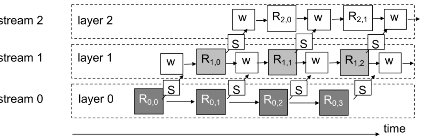
signaling splits each layer into multiple kernels across time steps. It should be noted that the kernels in the same stream have exactly the same weights (the same shades in Figure12). Hence, each kernel in the same stream has to reload the weights at each time step, which causes significant overhead.
The slowdown due to wasted weights reloading depends on the percentage of weights relative to the total memory consumption of the workload. The memory consumption of a RNN includes three parts: weights, inputs and temporal outputs. Both inputs and temporal outputs’ memory footprint scales linearly with the batch size. In practice, the batch size could be very small when running inference. As shown in Figure 13, using a batch size of 4 (as in [33]), the percentage of weights varies from 30% to 90% and is 68% on average. This indicates that preserving weights on-chip can greatly reduce off-chip memory traffic. It should be noted that this percentage of weights could stay the same even with larger batch sizes because a large batch could be split among multiple GPUs so that each GPU operates on a small batch size.
layer 0 layer 1 layer 2 stream 0 stream 1 stream 2 w w w R0,0 S S S R1,0 R2,0 R0,1 R1,1 R0,2 R0,3 w w S R1,2 S w S R2,1 w S time
Figure 12: Stream Implementation of wavefront parallelism. W: wait event. S: signal event.
Ri,t represents a kernelto compute a RNN cell at layer iand time step t.
0.3 0.7 0.8 0.7 0.9 0.68 0 0.1 0.2 0.3 0.4 0.5 0.6 0.7 0.8 0.9 1
Basic
GRU
LSTM
G-LSTM
P-LSTM
Average
Percentage of weights
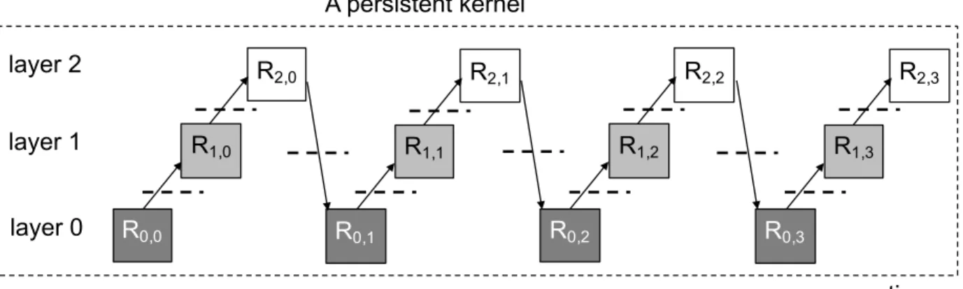
layer 0 layer 1 layer 2 A persistent kernel R0,0 R1,0 R2,0 R0,1 R1,1 R2,1 R0,2 R1,2 R2,2 R0,3 R1,3 R2,3 time
Figure 14: Persistent RNN. The dashed line indicates global barrier. Each Ri,t is computed by all TBs sequentially. 0.3 0.4 0.6 0.4 0.7 0.48 0 0.1 0.2 0.3 0.4 0.5 0.6 0.7 0.8
Basic
GRU
LSTM
G-LSTM
P-LSTM
Average
Utilization
3.2.3.4 Persistent implementations of RNNs Figure 14 shows a persistent imple-mentation of multi-layer RNNs [33]. The block in the figure represents a task that computes a RNN cell at a certain layer and a certain time step. A single kernel is launched and all TBs of that kernel are persistent on the GPU. All the thread blocks accomplish each task together, and the tasks are executed sequentially following the dependency arrows shown in the Figure 14. To preserve the weights on-chip, the weights of all layers have to be parti-tioned statically to each TB [33]. Specifically, the weights are stored using registers while the inputs and temporal results are stored in shared memory. This design requires that the GPU device have sufficient registers to store the entire weights of all layers. Hence, the batch size has to be carefully adjusted so that the kernel will not exceed the GPU’s capacity. The synchronization between thread blocks is global in nature, as shown as the dashed line in the figure. Such a global synchronization is implemented with atomic operations in assembly language [33, 25]. In summary, the kernel executes each block at each layer and each time step sequentially. It should be noted that although persistent RNN takes more time steps than the stream implementation depicted in Figure12, each time step is much shorter due to reusing on-chip weights. Hence, this design achieves great performance speedup compared to the stream based implementation. Obviously such a design doesn’t exploit the wavefront parallelism nature of RNNs. If the single task block in Figure 14 doesn’t require a large number of threads to compute, the GPU resources will be significantly underutilized. This actually occurs very frequently in real workloads for inference. As shown in Figure 15, on average, only 50% of the GPU computing resources are utilized for RNN inference. Higher GPU utilization could be achieved by exploiting wavefront parallelism.
3.3 ADDRESSING WARP SCHEDULING
3.3.1 Round Robin Warp Scheduling
Conventionally, a simple round robin (RR) scheduler is used to rotate among ready-to-issue warps on per cycle basis. Studies have shown that there are severe limitations in
such scheduling. RR may easily destroy the intra-warp data locality since a different warp is issued each cycle, slashing the L1 cache hit rates which can be performance critical to cache-sensitive applications.
3.3.2 Greedy Then Oldest Warp Scheduling
The poor locality problem of RR can be overcome by a Greedy-then-Oldest (GTO) algorithm where the scheduler greedily executes a warp until it stalls and then starts from the oldest ready warp in the SM.
3.3.3 CTA-aware two-level warp scheduling
RR gives each warp equal priority so that all warps proceed relatively uniformly. Many warps have fairly symmetric instruction sequences, due to the fact that they belong to the same Cooperative Thread Array (CTA, a block of closely coupled threads, or thread block). Hence, different warps tend to reach long latency operations, such as memory requests, roughly at the same time. Once all warps assigned to an SM are stalled, the SM becomes idle, degrading program performance. To overcome this limitation, a CTA-aware two-level warp scheduling (CATLS) scheme was proposed, in which warps are first divided into isolated groups. The scheduler prioritizes the warps in one group before switching to another group. Hence one group can advance much faster than other groups, creating skewed progress among warps and thus the SM can better hide stalls from a subset of warps.
4.0 EFFICIENT GLOBAL SYNCHRONIZATION
4.1 MOTIVATIONS FOR EFFICIENT GSYNC
Repeated kernel launching is the most widely used practice for implementing Gsync as it is easy to program. The split kernels are launched sequentially on the host side. To allow the CPU process to check convergence, a synchronization API call is used between kernels. Such API calls could account for more than 60% of execution time for short kernels [25]. In addition to the API call overhead, a more prominent problem of repeated kernel launching is data thrashing if there are data reuses across the split kernels.
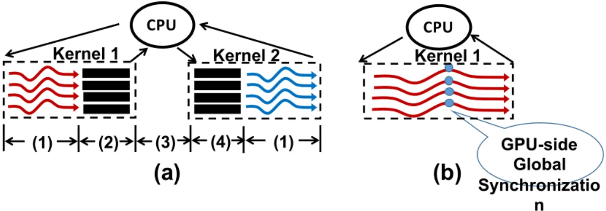
All on-chip data of the kernel preceding the Gsync including registers, shared memories and caches, are flushed upon exit, but have to be reloaded by the kernel following Gsync, as depicted in Figure 16(a). Such data thrashing results in idle time of cores and imposes high pressure on memory bandwidth. In fact, the thrashings could turn a compute-bound task into a memory-bound task [33]. The overhead of data thrashing may be acceptable for long executing kernels that amortize the overhead. However, in many contemporary machine learning applications where real-time response is required, such as real time object detection in self-driving cars, kernels are fairly short. For example, YOLO [50, 51] achieves 150 frames/seconds for object detection where the application running time is 6 ms and the average kernel running time is 200 µs. Due to the lack of hardware support for Gsync, kernel launching overhead plus data thrashing may become the performance bottleneck of an application [33, 52]. If those overheads are removed, the applications turn back to be compute-bound, and performance will scale well with more GPU nodes [33]. In cases where the API call overhead is small since cudaDeviceSynchronize() is not needed, data thrashing becomes a prominent problem. In many of these CNN kernels, the output of
GPU-side Global Synchronizatio n
(b)
(a)
CPUKernel 1 Kernel 2 Kernel 1
(1) (2) (3) (4) (1)
CPU
Figure 16: Global synchronization through (a) CPU-side API and repeated kernel launching: (1) kernel execution, (2) data flushing, (3) kernel launch overhead, (4) data reload; (b) the proposed GPU-side synchronization.
one kernel, such as feature maps [52], is the input of the next one. This output is flushed by one kernel but has to be loaded from global memory by the next kernel [52]. In other applications such as recurrent neural networks (RNN), abundant read-only data such as weights (for inference) are reused between kernels or even across many kernels. Repeated kernel launch would thrash those data across consecutive kernel executions, which is a critical performance bottleneck [33,52]. Combining kernels into one would eliminate such thrashing if no context switching is needed. Even with context switchings at the global barrier, we will show that keeping those reused data on-chip greatly reduces the amount of memory traffic for context switching. Figure 17 quantifies data reuse for two example applications: CNN and RNN. Both are miniature versions with smaller sizes for weights so that they can fit on-chip [33, 53]. As we can see, both have large portions of data reuse, 35% and 80% for CNN and RNN respectively. If this reused data is kept on-chip and no data thrashing occurs across the global barrier, an ideal speedup of 2× and 10× can be achieved over repeated kernel launch for CNN and RNN respectively.
0.35
0.8
0 0.5 1
Average reuse data
percentage
2
10
0 5 10 15Ideal Speedup
(a)
(b)
CNN
RNN
CNN
RNN
Figure 17: (a) Percentage of reused data across global barrier. (b) ideal speedup over repeated kernel launching if there is no data thrashing.
4.2 GPU-SIDE GLOBAL SYNCHRONIZATION API
Figure18shows examples of using globalSync(). Compared with the version in Figure7(a) using repeated kernel launching, the do-while loop including the termination check is moved into the kernel which is launched only once. Thus, the expensive cudaDeviceSynchronize() is invoked only once at the very end of the kernel. For neural network applications, an aggressive way is merging the entire network in
![Figure 4: GP100 Pascal GPU architecture [2].](https://thumb-us.123doks.com/thumbv2/123dok_us/387240.2542945/29.918.215.701.343.742/figure-gp-pascal-gpu-architecture.webp)