A model of Virtual Resource Scheduling in Cloud Computing and Its
Solution using EDAs
1
Jianfeng Zhao,
2Wenhua Zeng,
3Miu Liu,
4Guangming Li
1, First Author, 3Cognitive Science Department, Xiamen University, Xiamen, Fujian, China; Fujian
Key Laboratory of the Brain-like Intelligent Systems(Xiamen University), Xiamen, Fujian,
China, [email protected] [email protected]
*2,Corresponding Author, 4Fujian Key Laboratory of the Brain-like Intelligent Systems(Xiamen
University), Xiamen, Fujian, China; Software School of Xiamen University, Xiamen, Fujian,
China, [email protected] [email protected]
Abstract
Resource scheduling becomes more complex as the introduction of virtualization technology in cloud computing. This paper proposed a resource scheduling model using the concept of resource service ratio as an object function and employing Estimation of Distribution Algorithms (EDAs) to solve this model. In scheduling model, the resource was abstracted to nodes with attributes, the scheduling result was evaluated by resource service ratio instead of the tasks completion time. In EDAs, two novel factors were introduced, one was the iteration times of best individual unchanged for reducing the iteration time, and another was share probability for improving the fitness. In experiment, when the tasks number is between 5 and 55 and the load rate is between 0.5 and 1.5, comparing with Max-min algorithm, static algorithm and random algorithm, the resource service ratio of EDA algorithm is improved on average by at least 1.004 and at most 1.793 times.
Keywords
: Resource Scheduling, Cloud Computing, Estimation Of Distribution Algorithms1. Introduction
Scheduling problem is a widely existed problem in real world, for example, job-shop scheduling problem [1-3], scheduling in heterogeneous distributed systems [4], tasks scheduling in grid environment [5-7], vehicle scheduling [8, 9], and so on. This problem also exists in cloud computing environment, which plays an important role in cloud computing. Cloud computing [10] is a kind of novel larger-scale distributional computer center in recent year. Although the exactly definition is not clear [11-14], there were hundreds of products named cloud computing, such as Amazon EC2, IBM smart cloud, Google App Engine and so on. Different with the traditional computer center, virtualization is putted in cloud computing. The compute is sold as a service not a product due to the introduction of virtualization, which allows users to purchase compute on-demand.
However, the application of virtual technology makes the resource scheduling more complex compared with the tradition distributed computation. At the same time, the result of resource scheduling is critical for cloud computer in virtue of it decides the complete time of tasks. Therefore, the resource scheduling is a hot topic in cloud computing.
How to schedule resource in cloud computing environment, different methods were proposed by scholars. For example, Sotomayor [15] et. al proposed a resource lease manager called Haizea, which can act as a scheduling back end for OpenNebula [16]. Intel Corporation [17] investigated the shared resource contention problem for virtual machines, modeled the effect on each virtual machines’s performance. Kong [18] et. al proposed an efficient dynamic task scheduling scheme based on fuzzy logic systems for cloud computing, in which the availability and responsiveness preformance was formulated as a two-objective optimization. Song [19] et. al proposed a multi-tiered resource scheduling scheme which automatically provides on-demand capacities to the hosted services via resource flowing among VMs. Li [20] et. al propose a hybrid energy-efficient scheduling algorithm using dynamic migration.
All above the schuduling algorithms are the single task scheduling algorithm. The advantage of single task scheduling algorithm is that it’s easy to implement. The disavantage is that it cann’t implement the global infromation. This paper modeled the virtual resource scheduling on account of
the detailed analysis for the scheduling process in cloud computing and the requirment in reality. A novel concept named resource service rate was proposed and an optimazation model was established based on this concept. The Estimation of distribution algorithms (EDAs) was used to solve this problem, at the same time, two factors were introduced in EDAs for reducing the iteration times and improving the solution fitness. Comparing with the random algorithm, Static algorithm and Max-min algorithm, EDAs can solve this model and better resource service ratio was obtained.
2. Cloud computing and resource scheduling
Cloud computing is an popular noun in recently year. It was arguably first popularized in 2006 by Amazon’s Elastic Compute Cloud (EC2) [15] which is representative of Cloud computing. However, there is still no a widely accepted concept about cloud computing. After researching more than 20 definitions, Vaquero [10] et. al provided a definition that clouds are a large pool of easily usable and accessible virtualized resource (such as hardware, development platforms and/or services). Cloud computing becomes the elite among larger scale distributed computing methods thanks to its low-priced and usability brought by virtual technology in recent years.
a.Traditional distributed environment
b. Cloud computing environment
Figure 1. An illustration of resource scheduling
The introduction of virtualization technology brings huge benefits for cloud computing, whereas the challenge of resource scheduling is greater. Different with the traditional distributed system, a virtual resource layer is added as shown in figure 1. The traditional distributed scheduling decision system is illustrated in figure 1.a. At first, a task is received by scheduler, then schedules it to a physical device. It’s usually one-on-one scheduling, namely when a task is assigned to a physical device, if this device is buy, then the task waits until other users release this device. The scheduling in cloud computing is explained in figure 1.b. When the user’s requirements are received by system, the decision system assigns immediately a lot of virtual resource to user, which one task is assigned usually more than one virtual resource. Then the scheduler schedules the virtual resource to physical device, which one physical device is shared by more than one virtual resource. Therefore, the scheduling decision is more complex as the introduction virtual technology in cloud computing.
A mathematic definition for resource scheduling in cloud computing is shown as following.
Definition 1. The resource scheduling in cloud computing is that find a virtual resource set V = [vi], i = 1, 2, …, m and a best mapping L = {l1, l2, …, lm} for V to the physical resource set P = [pj], j = 1, 2, …, n in a certain time after the tasks set are received.
From the definition we know that the key of resource scheduling is to find a virtual resource set V and a mapping L. However, this problem is a hard problem.
Task
Device Device Device
Task Task … … Task Device VM VM VM Task Task VM VM VM Device … Device …
3. The resource scheduling model and its solution
3.1. The resource scheduling model
At first, this paper analyses the process of scheduling in cloud computing, then model for the virtual resource scheduling in cloud computing. Figure 2 describes the process of resource scheduling in cloud computing. At begin, the users access the cloud computing center by explorer or others remote terminal, put the tasks to cloud computing center. When the cloud computing center receives the tasks, the virtual resource will be assigned immediately by cloud system. Then the virtual resource is scheduled to the physical resource by scheduler.
Internet
Figure 2. The process of tasks requirement in cloud computing
In practice, the completion time of task is foremost concern of users when a task is put to cloud computing. So, many scholars [18, 19] proposed using completion time as the evaluation index to evaluate the scheduling result. However, the task completion time is related with the resource assigned to it, therefore, if employ the completion time as the evaluation index, the relationship of given resource and tasks completion time must be established. Whereas, it’s a hard work to establish this relationship thinks to different kind of tasks has the different running time when the same resource is obtained by the different kind of tasks. Various tasks have to be tested for established this relationship, it’s a hard work and the result is affected by the element of artificiality.
From the analysis we know that there is a positive correlation between the tasks completion time and assigned resource, namely, if a task obtain more resource, then the completion time is shorter. Inspired by this opinion, we proposed a concept called resource service ratio.
Define 2. Resource Service Ratio is the ratio of the assigned resource and required resource for a given task in cloud computing system.
Using resource service ratio to evaluate the scheduling result, the complexity of scheduling model will be simplified and the interference of experience function will be reduced. From the concept, we know that only the required resource and the assigned resource are necessary. It’s easy to obtain those two values in cloud system.
In the cloud computing system, the required resource of tasks, virtual resource and physical resource can be abstracted some nodes with attributes. In the cloud computing system, CPU, RAM and bandwidth are the common three attributes, this paper uses those three attributes to build model.
Set tasks set T = {ti}, i = 1, 2, …, m, where ti = (cti, mti, bti), cti, mti, bti is the value of CPU, RAM and bandwidth of task i; A virtual resource set is V = [vi], i = 1, 2, …, m, where, vi = (cvi, mvi, bvi), cvi, mvi, bvi is the value of CPU, RAM and bandwidth of virtual resource i; Similarly, the physical resource set is P = {pj}, j = 1, 2, …, n, where pj = (cpj, mpj, bpj), cpj, mpj, bpj is the remnant value of CPU, RAM and bandwidth of a physical device node.
A typical example of cloud computing is shown as table 1. The formal description of resource service ratio is as following.
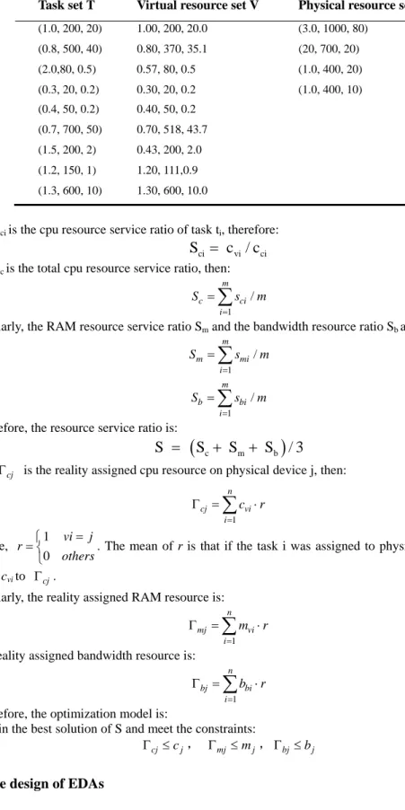
Table 1. The abstract task and resource
Task set T Virtual resource set V Physical resource set P
(1.0, 200, 20) 1.00, 200, 20.0 (3.0, 1000, 80) (0.8, 500, 40) 0.80, 370, 35.1 (20, 700, 20) (2.0,80, 0.5) 0.57, 80, 0.5 (1.0, 400, 20) (0.3, 20, 0.2) 0.30, 20, 0.2 (1.0, 400, 10) (0.4, 50, 0.2) 0.40, 50, 0.2 (0.7, 700, 50) 0.70, 518, 43.7 (1.5, 200, 2) 0.43, 200, 2.0 (1.2, 150, 1) 1.20, 111,0.9 (1.3, 600, 10) 1.30, 600, 10.0
Set Sci is the cpu resource service ratio of task ti, therefore: ci vi ci
S
c / c
(1)Set Sc is the total cpu resource service ratio, then:
1 / m c ci i S s m
(2)Similarly, the RAM resource service ratio Sm and the bandwidth resource ratio Sb are:
1 / m m mi i S s m
(3) 1 / m b bi i S s m
(4)Therefore, the resource service ratio is:
c m b
S
S
S
S
/ 3
(5)Set cj is the reality assigned cpu resource on physical device j, then:
1 n cj vi i c r
(6) where, 1 0 vi j r others . The mean of r is that if the task i was assigned to physical device j, then
sum the cvito cj.
Similarly, the reality assigned RAM resource is:
1 n mj vi i m r
(7)the reality assigned bandwidth resource is:
1 n bj bi i b r
(8)Therefore, the optimization model is:
Obtain the best solution of S and meet the constraints: cj cj
, mj mj, bj bj (9)
3.2. The design of EDAs
is that find out the object function extreme value by iterating people. The object function is formula 5 in this paper and the extreme value of S is the maximum value of S. People consist of individuals, an individual correspond a solution of object function. Iteration is generating next people using current people according some rules. Different evolutional algorithms have different rules.
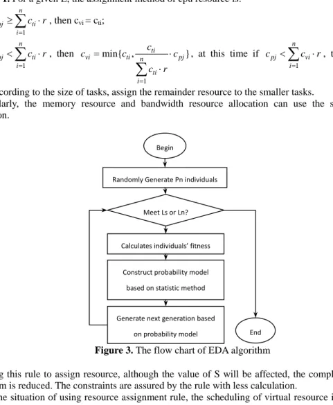
A whole EDAs evolutional algorithm flow chart is shown as figure 3. At first, generate the people randomly, then calculate the fitness of individuals, at last, generate the next generation based on the probability model, namely sample every code of every individuals depend on this probability model. Therefore, that there are two key points in EDAs algorithm: 1) the individual code; 2) the probability model. We will introduce these two points separately.
3.2.1. The individual code
From the definite 1 we know that: the resource scheduling in cloud computing is to find V and L. For a given V and L, firstly it’s necessary to judge whether the V meet the constraints in optimization model, then obtain the resource service ratio S by solution according with formula 5. Solving Constrained optimization problems (COPs) has become an important research area of evolutionary computation in recent years [22]. This paper uses the following rule to give the corresponding V:
Rule 1. For a given L, the assignment method of cpu resource is: if 1 n pj ti i c c r
, then cvi = cti; if 1 n pj ti i c c r
, then 1 min{ , ti } vi ti n pj ti i c c c c c r
, at this time if 1 n pj vi i c c r
, then sort thetasks according to the size of tasks, assign the remainder resource to the smaller tasks.
Similarly, the memory resource and bandwidth resource allocation can use the same rule to allocation.
Figure 3. The flow chart of EDA algorithm
Using this rule to assign resource, although the value of S will be affected, the complex degree of algorithm is reduced. The constraints are assured by the rule with less calculation.
On the situation of using resource assignment rule, the scheduling of virtual resource is changed to find a mapping L. Therefore, for a given cloud computing system, we identify each physical node, there is an ID corresponding with each physical device. Set the ID set is D, then for a task set T, there is a code L = { li|li∈D } corresponding with it. For example, set |T| = m, m = 8, then L = {1,3,1,5,9,3,5,7}
Begin
Randomly Generate Pn individuals
Calculates individuals’ fitness Meet Ls or Ln?
Construct probability model based on statistic method
Generate next generation based
is a mapping of T, which represents that the first task is assigned to physical node 1, the second task is assigned to physical node 3, and so on.
3.2.2. The probability model
The main idea of this model in this paper is from Univariate Marginal Distribution Algorithm (UMDA) [21], namely select some best individuals, then using those individuals to construct probability model. Set Pn is the number of individuals in people, Sp is the selection possibility, namely how much individuals should be selected from the people. Therefore the probability model is:
1 1 1
'( )
'( |
)
'( )
(
|
)
n S l l l i i N S j i i l n j ip
x
p x D
p
x
X
x D
N
(10)where, n is the number of object functions, as there is only one fitness function in this paper, so
n=1;
*
N
Pn Sp
(11)1
(
|
)
0
i i S j i i lX
x
X
x D
others
(12) s lD
is the sub-people selected from l generation which includes N individuals.This paper introduces a parameter Pm to the EDAs algorithm. The main purpose of Pm is to avoid the gene with lower possibility being weeded out too early. From the formula 10 we know that if a gene doesn’t appear in once iteration, then the appearance possibility of this gene in next generation is 0. For avoiding this unreasonable situation, we introduce shared factor Pm in EDAs. As shown in formula 13, if there is a gene doesn’t appear in once iteration, then the appearance possibility of this gene in next generation is Pm/m.
( )
/
(1
) *
'( )
l m m l
p x
p
m
p
p
x
(13)The algorithm of generating next generation people is shown as following.
Alg. 1 The algorithm of constructing probability model in EDAs
cal_poss(selected sub-people
D
ls){ for(i<1; i<n; i++){for(j<1; j<m;i++){
possibility_model(i,j)=calculate depending on formula 10 and 13; }
}
return possibility_model; }
Alg. 2 The algorithm of generating next generation people in EDAs
Eda(People) {
Sorting the individuals according with the individual fitness in people; Select the top Sp*Pn individuals to construct
D
ls;possibility_model = cal_poss(
D
ls); for(i=1;i<Pn;i++){for(j=1; j<the length of individual; i++){
next_people(i,j) = sample from the probability model; }
}
}
The parameters and their values are shown in table 2.
Table 2. The parameters, their meaning and value in EDA
Parameters meaning value
Ln The most iteration time 150 Ls unchanged iteration number of best individual 70
Pn the number of people 50
Sp ratio of chosen 0.15
Pm minimal possibility shared by all services 0.2
4. The experiment and discussion
4.1. The environment of experiment
For verifying the result of algorithms without the interference of the noise, this paper uses the simulator to test. How to simulate a cloud computing? In practical, the scheduling result is affected by two points: one is the number of tasks arrived at the same time; another is ratio of required resource and physical resource named load ratio. If the number of tasks arrived at the same time is large the scheduling will become more complex. Besides if the load ratio is large, it means there are many tasks can’t be service. In view of those two points, we give some fixed parameters to represent an existed cloud computing system at first, then we adjust the number of arrived tasks and the load ratio to simulate the different sense of resource scheduling in cloud computing system.
In the simulator, the generation scopes of physical resource are: CPU (0.5~1.5), RAM (500~1500), bandwidth (1~9), the quantity of physical resource is 20. The generation of tasks is decided by two points: one is the number of physical resource and the number of tasks; another is the load ratio. So the generation method of tasks is shown as formula 14.
* ( ( ) * / ) * 2
resourcerandom sum p ratio m (14)
Where, resource is a attribute of the task, such as CPU. random is a random. sum(p) is the sum of physical resource corresponding with the attribute of the task, namely
1
sum p =
(
)
n i ip attr
. ratiois the ratio of the total required resource and the total physical resource, m is the number of tasks. For example, set we want to random generate the CPU attribute of a tasks set. For a given task, set the random is 0.6, sum(p) is 20.7, which is sum of all physical resource CPU value, the ratio is 0.9, the
m is 40, those two parameters value are appointed by experiment, therefore, the CPU value of a task is 0.5778.
The design of other algorithms: 1) Max-min algorithm
Principle: For a given task, return the physical resource with the largest resource ratio as the scheduling solution. The pseudo code is shown as following.
Alg. 3 The pseudo code of Max-min
Solution L Max_min(t,p){ for (ti∈t) {
for (pi∈p) {
res=ti.cpu/pi.cpu + ti.RAM/pi.RAM + ti.bandwidth/pi.bandwidth; Record the largest res as the physical resource assigned to ti; }
L(i) = ti.serial; }
return L; }
2) Static algorithm
Principle: Assign the task to the physical resource with same ID number. If the task ID is lager than the largest physical resource ID, then use the remainder of task ID divided the largest physical resource ID, namely the scheduling solution is similarly with (1, 2, …).
3) Random algorithm
Principle: Randomly assign the task to physical resource.
4.2. Experiment result and discuss
4.2.1. Solve an instanceTable 3 shows the solution of the table 1 using different algorithms. From the table we know that the resource service ratio of EDA algorithm is better than other three algorithms. Table 4 displays the total virtual resource assigned to the tasks set by different algorithms. From the table 4 we know that EDA can maximize the efficiency of physical resource.
Table 3. The solutions of resource the instance in table 1 using different algorithms
Alg. Solution s sc sm sb
EDA 3 1 4 2 2 1 4 1 2 0.90 0.84 0.91 0.95
Max-min 1 1 2 2 3 1 2 3 4 0.84 0.73 0.87 0.91
Static 1 2 3 4 1 2 3 4 1 0.83 0.76 0.91 0.83
Random 1 1 4 3 2 1 2 1 2 0.80 0.74 0.78 0.87
Table 4. The total virtual resource assigned to tasks set by different algorithms
Attribute EDA Max-min Static Random
CPU 6.7 6.5 6.2 6.3
RAM 2150 1900 2000 1800
Bandwidth 112.9 93.9 53.9 92.9
Table 5. The concrete assignment of each physical device with different algorithms
No. EDA Max-min Static Random P set
1 (2.70, 1000.00, 80.00) (2.50, 1000.00, 80.00) (2.70, 850.00, 30.20) (3.00, 1000.00, 80.00) (3.0, 1000, 80) 2 (2.00, 670.00, 10.40) (2.00, 300.00, 2.70) (1.50, 700.00, 20.00) (2.00, 700.00, 12.20) (2.0, 700, 20) 3 (1.00, 200.00, 20.00) (1.00, 200.00, 1.20) (1.00, 280.00, 2.50) (0.30, 20.00, 0.20) (1.0, 400, 20) 4 (1.00, 280.00, 2.50) (1.00, 400.00, 10.00) (1.00, 170.00, 1.20) (1.00, 80.00, 0.50) (1.0, 400, 10)
Table 6. The concrete assignment of each task with different algorithms
No. EDA Max-min Static Random T set
1 (1.00, 200.00, 20.00) (1.00, 142.86, 14.55) (1.00, 200.00, 20.00) (0.81, 129.03, 14.41) (1.0, 200, 20) 2 (0.80, 370.37, 35.16) (0.80, 357.14, 29.09) (0.80, 291.67, 8.89) (0.65, 322.58, 28.83) (0.8, 500, 40) 3 (0.57, 80.00, 0.50) (1.05, 80.00, 0.50) (0.57, 80.00, 0.50) (1.00, 80.00, 0.50) (2.0,80, 0.5) 4 (0.30, 20.00, 0.20) (0.16, 20.00, 0.20) (0.20, 20.00, 0.20) (0.30, 20.00, 0.20) (0.3, 20, 0.2) 5 (0.40, 50.00, 0.20) (0.25, 50.00, 0.20) (0.40, 50.00, 0.20) (0.25, 41.18, 0.20) (0.4, 50, 0.2) 6 (0.70, 518.52, 43.96) (0.70, 500.00, 36.36) (0.70, 408.33, 11.11) (0.57, 451.61, 36.04) (0.7, 700, 50) 7 (0.43, 200.00, 2.00) (0.79, 200.00, 2.00) (0.43, 200.00, 2.00) (0.94, 164.71, 2.00) (1.5, 200, 2) 8 (1.20, 111.11, 0.88) (0.75, 150.00, 1.00) (0.80, 150.00, 1.00) (0.97, 96.77, 0.72) (1.2, 150, 1) 9 (1.30, 600.00, 10.00) (1.00, 400.00,10.00) (1.30, 600.00, 10.00) (0.81, 494.12, 10.00) (1.3, 600, 10)
Table 5 shows the concrete assignment of physical devices. For physical devices, the max value of assigned resource can’t be over the devices value. If the assigned resource is greater than devices value,
the performance of devices will drop down. From the table 5, all algorithms aren’t greater than the devices value.
Table 6 shows the concrete value assigned to each task. Ideally, every task can obtain the resource they needs. However, it’s hard to reach this goal for the constraint of physical devices. From the table we know that EDA algorithm is better than other algorithms due to it can more fulfill the tasks.
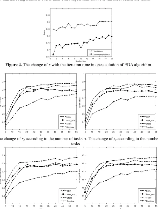
Figure 4. The change of s with the iteration time in once solution of EDA algorithm
a. The change of sc according to the number of tasks b. The change of sr according to the number of
tasks
c. The change of sb according to the number of tasks d. The change of s according to the number of tasks
Figure 5. The change of object function according to the number of tasks
Figure 4 displays once iteration process of EDA algorithm. The abscissa axis is iteration time and the vertical axis is the value of s, namely the resource service ratio. From the figure we know that the iteration time is 20. As the iteration time increasing, the average fitness of people increases rapidly firstly, then increases slowly with fluctuated. The best individual fitness always fluctuates as the iteration time increasing and obtains best value at 7th iteration time. The reason is that the problem
scale is small (9^4), so the iteration time is small and the fitness of best individual is little changed.
4.2.2. Algorithm comparison on different number of tasks
Figure 5 shows the variety of s value as the task set including different number of tasks. The s value is average value after running 25 times. In the experiment, the load ratio is 1.0, the physical resource is generated randomly and the task set is generated depending on the formula 14. It can be observed that EDA is better than other algorithms. Specially, EDA algorithm is obviously better than other algorithms when the tasks are small. If the load ratio is fixed, the total required resource is fixed for a given cloud system, therefore, the required resource of single task will be larger when the number of tasks is small. The scheduling will become more complex and the advantage of EDA algorithm become more obvious on this situation. From calculation it can be obtained that the average resource service ration s of EDA algorithm is 1.060, 1.039, 1.793 times respectively of Max-min algorithm, static algorithm and random algorithm.
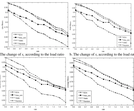
a. The change of sc according to the load ratio b. The change of sr according to the load ratio
c. The change of sb according to the load ratio d. The change of s according to the load ratio Figure 6. The change of object function according to the load ratio
4.2.3. Algorithm comparison on different load ratio
Then, we will study the scheduling on different load ratio. In this situation, as the tasks number is often more than devices number in reality, set m=20, n=40. Figure 6 shows the average result of s after running 25 times when the load ration from 0.5 to 1.5. From the figure we can see that s of EDA algorithm is 1 when the load ratio is low, s descends as the load ratio increasing. The reason is there are more tasks can’t be service as the load ratio increasing. From the figure it also can be concluded that EDA algorithm is better than other algorithms. According the calculation, the average s of EDA algorithm is better 1.065, 1.004, 1.177 times than Max-min algorithm, static algorithm and random algorithm.
5. Conclusion
This paper studies the resource scheduling algorithm in cloud computing, proposes a resource scheduling optimization model using resource service as the object function and employs EDAs to solve this model. At first, a detail analysis of resource scheduling on cloud computing environment is given, using resource service replaces completion time to evaluate the scheduling result, models the resource scheduling based on this concept; then, using EDA algorithm to solve this problem; at last, an experiment is designed to verify the feasible of this model. In experiment, a small instantiate is solved to verify the correctness of the model and learn the solving process in detail. Besides of those, compares with the Max-min algorithm, static algorithm and random algorithm. The result shows: EDA algorithm is averagely better than other algorithms at least 1.004 and at most 1.793 when the number of tasks from 5 to 55 or the load ratio from 0.5 to 1.5.
6. Acknowledgment
This work was supported by the Fujian Key Laboratory of the Brain-like Intelligent Systems (Xiamen University), P. R. China, the National Natural Science Foundation of China (Grant No. 60903129, 60975084, 30900328).
7. Reference
[1] Rui Zhang, "A genetic local search algorithm based on insertion neighborhood for the job shop scheduling problem," Advances in Information Sciences and Service Sciences, vol. 3, no. 5, pp. 117-125, 2011.
[2] Song Cun-Li, Liu Xiao-Bing, Wang Wei,Xin Bai, "A hybrid particle swarm optimization algorithm for job-shop scheduling problem," International Journal of Advancements in Computing Technology,vol. 3, no. 4, pp. 79-88, 2011.
[3] Zhang Rui, "A particle swarm optimization algorithm based on local perturbations for the job shop scheduling problem," International Journal of Advancements in Computing Technology,vol. 3, no. 4, pp. 256-264, 2011.
[4] Jing Weipeng, Liu Yaqiu,Wu Qu, "Communication-aware fault-tolerant scheduling strategy for precedence constrained tasks in heterogeneous distributed systems," International Journal of Digital Content Technology and its Applications,vol. 5, no. 6, pp. 252-260, 2011.
[5] Xun-Yi Ren, Zheng-hua Qi, Ru-chuan Wang,Xiao-dong Ma, "Rough set and A* based tasks scheduling in gird environment," International Journal of Digital Content Technology and its Applications,vol. 4, no. 4, pp. 193-198, 2010.
[6] Dr.K.Vivekanandan, D.Ramyachitra, B.Anbu, "Artificial bee colony algorithm for grid scheduling," Journal of Convergence Information Technology,vol. 6, no. 7, pp. 328-339, 2011. [7] Song Kunfang, Ruan Shufen,Jiang Minghua, "A flexible grid task scheduling algorithm based on
QoS similarity," Journal of Convergence Information Technology,vol. 5, no. 7, pp. 21-27, 2010. [8] Chen Jia-wei, Zhang Yuan-Biao,Wang Geng-Jia, "A new algorithm for a fuzzy vehicle routing and
scheduling problem: Imperialist competitive algorithm," Journal of Convergence Information Technology,vol. 6, no. 7, pp. 303-311, 2011.
[9] Wang Geng-jia, Zhang Yuan-Biao,Chen Jia-Wei, "A novel algorithm to solve the vehicle routing problem with time windows: Imperialist competitive algorithm," Advances in Information Sciences and Service Sciences, vol. 3, no. 5, pp. 108-116, 2011.
[10]Luis M. Vaquero, Luis Rodero-Merino, Juan Caceres, Maik Lindner, "A break in the clouds: towards a cloud definition," ACM SIGCOMM Computer Communication Review, vol. 39, no. 1, pp. 50-55, 2008.
[11]Armbrust Michael, Fox Armando, Griffith Rean, Joseph Anthony D., Katz Randy H., Konwinski Andrew, Lee Gunho, Patterson David A., Rabkin Ariel, Stoica Ion, Zaharia Matei, "Above the clouds: A berkeley view of cloud computing," EECS Department, University of California, Berkeley, Tech. Rep. UCB/EECS-2009-28, 2009.
[12] Erik Brynjolfsson, Paul Hofmann, John Jordan, "Cloud Computing and Electricity: Beyond the Utility Model," Communications of the Acm, vol. 53, no. 5, pp. 32-34, 2010.
[13] Rajkumar Buyya, Chee Shin Yeo, Srikumar Venugopal, James Broberg, Ivona Brandic, "Cloud computing and emerging IT platforms: Vision, hype, and reality for delivering computing as the 5th utility," Future Generation Computer Systems-the International Journal of Grid Computing-Theory Methods and Applications, vol. 25, no. 6, pp. 599-616, 2009.
[14] Michael Armbrust, Armando Fox, Rean Griffith, Anthony D. Joseph, Randy Katz, Andy Konwinski, Gunho Lee, David Patterson, Ariel Rabkin, Ion Stoica, Matei Zaharia, "A View of Cloud Computing," Communications of the Acm, vol. 53, no. 4, pp. 50-58, 2010.
[15] Borja Sotomayor,, Rubén S. Montero, Ignacio M. Llorente, Ian Foster, "Virtual Infrastructure Management in Private and Hybrid Clouds," Ieee Internet Computing, vol. 13, no. 5, pp. 14-22, 2009.
[16] Peter Sempolinski, Douglas Thain, "A Comparison and Critique of Eucalyptus, OpenNebula and Nimbus," in Cloud Computing Technology and Science (CloudCom), 2010 IEEE Second International Conference on, pp. 417-426, 2010.
[17] Ravi Iyer, Ramesh Illikkal, Omesh Tickoo, Li Zhao, Padma Apparao, Don Newell, "VM3: Measuring, modeling and managing VM shared resources," Computer Networks, vol. 53, no. 17, pp. 2873-2887, 2009.
[18] Xiangzhen Kong, Chuang Lin, Yixin Jiang, Wei Yan, Xiaowen Chu, "Efficient dynamic task scheduling in virtualized data centers with fuzzy prediction," Journal of Network and Computer Applications, vol. 34, no. 4, pp. 1068-1077, 2011.
[19] Song Ying, Wang Hui, Li Yaqiong, Feng Binquan,Sun Yuzhong, "Multi-Tiered On-Demand Resource Scheduling for VM-Based Data Center," in Proceedings of the 2009 9th IEEE/ACM International Symposium on Cluster Computing and the Grid, pp. 148-155, 2009.
[20] Li Jiandun, Peng Junjie, Zhang Wu, "A scheduling algorithm for private clouds," Journal of Convergence Information Technology, vol. 6, no. 7, pp. 1-9, 2011.
[21] Zhou Shude, Sun Zengqi, "A survey on Estimation of Distribution Algorithms," ACTA automatic sinica, vol. 33, no. 2, pp. 113-125, 2007.
[22] Wang Yong, Cai Zixing, Zhou Yuren, Xiao Chixin, "Constrained optimization evolutionary algorithms," Journal of Software,vol. 20, no. 1, pp. 11-29, 2009.