H a o , Yu
C r o w d Ab n o r m al B e h a vio u r D e t e c tio n a n d An aly si s Or i g i n a l C i t a t i o n
H a o , Yu ( 2 0 1 9 ) C r o w d Ab n o r m al B e h a vio u r D e t e c ti o n a n d An aly si s. Do c t o r a l t h e si s, U n iv e r si ty of H u d d e r s fi el d .
T hi s v e r si o n is a v ail a bl e a t h t t p :// e p r i n t s . h u d . a c . u k/i d/ e p r i n t/ 3 5 1 0 0 /
T h e U n iv e r si ty R e p o si t o r y is a d i gi t al c oll e c tio n of t h e r e s e a r c h o u t p u t of t h e U niv e r si ty, a v ail a bl e o n O p e n Acc e s s . C o p y ri g h t a n d M o r al Ri g h t s fo r t h e it e m s
o n t hi s si t e a r e r e t ai n e d b y t h e i n divi d u a l a u t h o r a n d / o r o t h e r c o p y ri g h t o w n e r s .
U s e r s m a y a c c e s s full it e m s fr e e of c h a r g e ; c o pi e s of f ull t e x t it e m s g e n e r a lly c a n b e r e p r o d u c e d , d i s pl ay e d o r p e rf o r m e d a n d g iv e n t o t hi r d p a r ti e s i n a n y fo r m a t o r m e d i u m fo r p e r s o n al r e s e a r c h o r s t u dy, e d u c a ti o n al o r n o t-fo r-p r ofi t p u r p o s e s wi t h o u t p r i o r p e r m i s sio n o r c h a r g e , p r o vi d e d :
• T h e a u t h o r s , ti tl e a n d f ull b i blio g r a p h i c d e t ail s is c r e d i t e d in a n y c o p y; • A h y p e r li n k a n d / o r U RL is in cl u d e d fo r t h e o ri gi n al m e t a d a t a p a g e ; a n d • T h e c o n t e n t is n o t c h a n g e d i n a n y w ay.
F o r m o r e i nfo r m a t io n , in cl u di n g o u r p olicy a n d s u b m i s sio n p r o c e d u r e , p l e a s e c o n t a c t t h e R e p o si t o r y Te a m a t : E. m a il b ox@ h u d . a c. u k .
Crowd Abnormal Behaviour
Detection and Analysis
Yu Hao
Submitted for the Degree of Doctor of Philosophy
From the University of Huddersfield
School of Computing and Engineering University of Huddersfield Queensgate, Huddersfield, HD1 3DH
I
Copyright Statement
I. The author of this thesis (including any appendices and/or schedules to this thesis) owns any copyright in it (the “Copyright”) and he has given The University of
Huddersfield the right to use such Copyright for any administrative, promotional, educational and/or teaching purposes.
II. Copies of this thesis, either in full or in extracts, may be made only in accordance with the regulations of the University Library. Details of these regulations may be obtained from the Librarian. This page must form part of any such copies made.
III. The ownership of any patents, designs, trademarks and any and all other intellectual property rights except for the Copyright (the “Intellectual Property Rights”) and any reproductions of copyright works, for example graphs and tables (“Reproductions”),
which may be described in this thesis, may not be owned by the author and may be owned by third parties. Such Intellectual Property Rights and Reproductions cannot and must not be made available for use without the prior written permission of the owner(s) of the relevant Intellectual Property Rights and/or Reproductions.
II
Acknowledgements
I would like to thank my supervisor, Professor Zhijie Xu. He provided me advices, inspirations and patiently instructions during this PhD program with the length of five years. I’m impressed by his persistence and responsibility of helping his students, and will take him as an example as a lecturer of Xi’an University of Posts and Telecommunications in China.
I would like to thank Professor Ying Liu and Professor Jiulun Fan in China, as well as Xi’an University of Posts and Telecommunications for providing the funding to support this program.
I would also like to thank my wife and parents for taking care of our newly born son while I’m at UK.
III
Abstract
The analysis and understanding of abnormal behaviours in human crowds is a challenging task in pattern recognition and computer vision. First of all, the semantic definition of the term “crowd” is ambiguous. Secondly, the taxonomy of crowd behaviours is usually rudimentary and intrinsically complicated. How to identify and construct effective features for crowd behaviour classification is a prominent challenge. Thirdly, the acquisition of suitable video for crowd analysis is another critical problem.
In order to address those issues, a categorization model for abnormal behaviour types is defined according to the state-of-the-art. In the novel taxonomy of crowd behaviour, eight types of crowd behaviours are defined based on the key visual patterns. An enhanced social force-based model is proposed to achieve the visual realism in crowd simulation, hence to generate customizable videos for crowd analysis. The proposed model consists of a long-term behavior control model based on A-star path finding algorithm and a short-term interaction handling model based on the enhanced social force. The proposed simulation approach produced all the crowd behaviours in the new taxonomy for the training and testing of the detection procedure. On the aspect of feature engineering, an innovative signature is devised for assisting the segmentation of crowd in both low and high density. The signature is modelled with derived features from Grey-Level Co-occurrence Matrix. Another major breakthrough is an effective approach for efficiently extracting spatial temporal information based on the information entropy theory and Gabor background subtraction. The extraction approach is capable of obtaining the texture with most motion information, which could help the detection approach to achieve the real-time processing.
Overall, these contributions have supported the crucial components in a pipeline of abnormal crowd behaviour detecting process. This process is consisted of crowd behaviour taxonomy, crowd video generation, crowd segmentation and crowd abnormal behaviour detection. Experiments for each component show promising results, and proved the accessibility of the proposed approaches.
IV
List of Publications
[1] Yu Hao, Zhijie Xu, Ying Liu, Jing Wang, Jiulun Fan. Unsupervised Pedestrian Sample
Extraction for Model Training. In the 13th International Conference on Computer Graphics,
Visualization, Computer Vision and Image Processing, 2019
[2] Yu Hao, Zhijie Xu, Ying Liu, Jing Wang, Jiulun Fan. Crowd Synthesis Based on Hybrid
Simulation Rules for Complex Behaviour Analysis. In Proceedings of the 24th International
Conference on Automation & Computing, 2018
[3] Yu Hao, Zhijie Xu, Ying Liu, Jing Wang, Jiulun Fan. A Graphical Simulator for Modeling
Complex Crowd Behaviours. In 22nd International Conference Information Visualization, 2018
[4] Yu Hao, Zhijie Xu, Ying Liu, Jing Wang, Jiulun Fan. An Innovative Crowd Segmentation
Approach based on Social Force. The Twelfth International Conference on Advanced
Engineering Computing and Applications in Sciences, 2018
[5] Yu Hao, Zhijie Xu, Ying Liu, Jing Wang, Jiulun Fan. Extracting Spatio-temporal Texture
Signatures for Crowd Abnormality Detection. In Proceedings of the 23th International
Conference on Automation & Computing, 2017
[6] Yu Hao, Zhijie Xu, Ying Liu, Jing Wang, Jiulun Fan. An Effective Video Processing Pipeline
for Crowd Pattern Analysis. In Proceedings of the 23th International Conference on Automation
& Computing, 2017
[7] Yu Hao, Zhijie Xu, Ying Liu, Jing Wang, Jiulun Fan. Effective Crowd Anomaly Detection
through Spatio-Temporal Texture Analysis. In International Journal of Automation and
Computing, 2018
[8] Yu Hao, Zhijie Xu, Ying Liu, Jing Wang, Jiulun Fan. An Approach to Detect Crowd Panic
Behaviour using Flow-based Feature. In Proceedings of the 22th International Conference on
V
List of Symbols & Abbreviations
ASM Angular Second Moment
BOW Bag of Word
EM Expectation Maximization
FCNN Fully Convolutional Neural Network
GLCM Grey Level Co-occurrence Matrix
GAF Group Attraction Force
HMM Hidden Markov Model
HOG Histogram of Oriented Gradient
HOT Histogram of Oriented Tracklets
HS Horn and Schunck Optical Flow
IEP Interaction Energy Potentials
IDM Inverse Different Moment
KNN K Nearest Neighbor
KLT Kanade-Lucas-Tomasi Feature Tracker
LDA Latent Dirichlet Allocation
LBP Linear Binary Pattern
LSTM Long Short-Term Memory
LK Lucas and Kanade Optical Flow
MDT Mixture of Dynamic Textures
MBH Motion Boundary Histogram
NMF Non-Negative Matrix Factorization
PSO Particle Swarm Optimization
PLE Principle of Least Effort
ROIs Regions-of-Interest
SIFT Scale-invariant feature transform
SFM Social Force Model
STT Spatio-Temporal Texture
STV Spatio-Temporal Volume
VI
List of Figures
Figure 1-1. Research field hierarchy ... 3
Figure 1-2. Examples of Behaviour Analysis on Individual Behaviours and Crowd Behaviours .... 4
Figure 1-3. The Procedure of Crowd Analysis ... 5
Figure 2-1. Taxonomy of Image Features in Computer Vision ... 10
Figure 2-2. Extraction Process of HOG Feature ... 13
Figure 2-3. Hough Transform Boundary Detection ... 14
Figure 2-4. Taxonomy of Video Based Features ... 16
Figure 2-5. (a) Moving but without Optical Flow. (b) Static but with Optical Flow ... 19
Figure 2-6. The STV Modelling and STT Extraction ... 20
Figure 2-7. Acceleration, Repulsive and Obstacle Avoidance Forces in SFM ... 21
Figure 2-8. Process of Modelling Social Force ... 23
Figure 2-9. General Procedure of Conventional Approach ... 24
Figure 2-10. Procedure of DT Behaviour Recognition ... 26
Figure 2-11. Taxonomy of Deep Learning Approaches... 29
Figure 2-12. General Procedure of Deep Learning ... 29
Figure 2-13. Rules of Boids Behavioural Model ... 33
Figure 2-14. Sample Iterations of A Cellular Automata ... 35
Figure 2-15. Structure of Block-Based Approach ... 36
Figure 2-16. A Three-Layer Structure of Hybrid Crowd Simulation ... 37
VII
Figure 3-1. Taxonomy of Crowd Behaviours ... 43
Figure 3-2. Sub-Phenomena in Bottleneck and Fountainhead ... 44
Figure 3-3. Lane Effect of Crowd ... 45
Figure 4-1. The Proposed STT Extraction Approach ... 49
Figure 4-2. Images with Corresponding Information Entropy Value ... 52
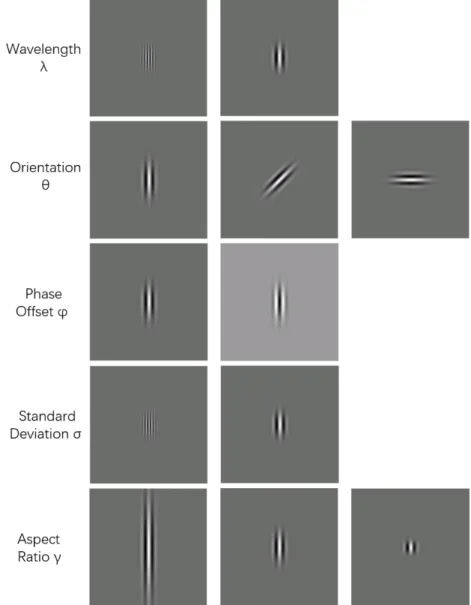
Figure 4-3. The Influence to Gabor Kernel by Changing Values of Parameters ... 54
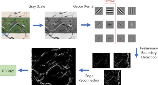
Figure 4-4. Procedure of Boundary Detection with Gabor Filter ... 54
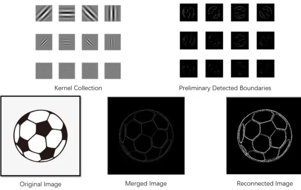
Figure 4-5. Results of each Processing Phase in Gabor Boundary Detection ... 55
Figure 4-6. Entropy Values of Random STTs... 57
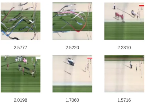
Figure 4-7. Selected STTs from Various Video Footages ... 57
Figure 4-8. The Parallel Lines in STT which Influence the Entropy Estimation ... 58
Figure 4-9. The Procedure of Improved STT Selection Approach ... 59
Figure 4-10. Gabor Filtering Results along Eight Directions ... 60
Figure 4-11. Comparison between Results with Eight and Six Kernel Functions ... 61
Figure 4-12. Motion Information in the STT ... 62
Figure 4-13. Crowd Panic Dispersing Detection Result ... 64
Figure 5-1. Taxonomy of Texture Extraction Approaches ... 69
Figure 5-2. GLCM Extraction ... 72
Figure 5-3. K-Nearest Neighbor Classification... 74
Figure 5-4. Support Vectors, Decision Boundary and Interval Boundary in SVM ... 76
Figure 5-5. Structure of BP Neural Network ... 77
VIII
Figure 5-7. Trends of GLCM Patterns along Time ... 84
Figure 5-8. The Proposed Framework of Panic Crowd Behaviour Detection Approach ... 86
Figure 5-9. A Comparison of Optical Flows before and after the Neighborhood Average Procedure ... 87
Figure 5-10. Changing of Magnitude in Panic Event ... 88
Figure 5-11. Difference Values S between S and A Value for Each Frame ... 89
Figure 5-12. Detection Results using the Proposed Framework ... 90
Figure 6-1. The Framework of Proposed Crowd Synthesis Technique ... 92
Figure 6-2. Flow Chart of A-Star Path Finding Algorithm ... 95
Figure 6-3. The Repulsive Affected by Personal Space ... 97
Figure 6-4. The Repulsive Force Affected by Relative Velocity ... 98
Figure 6-5. The Field Perception and the Impact on Result with Different Parameters ... 99
Figure 6-6. Comparison between Agents’ Distribution and Extracted Grouping Centers ... 102
Figure 6-7. Comparison between Ground Truth and Segmentation Result ... 102
Figure 6-8. The Framework of the Proposed Crowd Prediction Approach ... 104
Figure 7-1. Normal and Abnormal Snapshots from UMN Dataset ... 108
Figure 7-2. Snapshots from UCSD Dataset and the Labelled Anomalies ... 109
Figure 7-3. Snapshots from Forensic Video Dataset ... 110
Figure 7-4. Snapshots from Dataset with Extreme High Density ... 111
Figure 7-5. Structure of Proposed Classification Approach... 112
Figure 7-6. Detection Result using GLCM Signature and KNN ... 113
IX
Figure 7-8. Comparison of Detection Results on Panic Dispersing ... 115
Figure 7-9. Detection Result of the Proposed Change Detection Approach ... 117
Figure 7-10. Snapshots of Simulation Results using Proposed Approach ... 121
Figure 7-11. STTs Comparison between Simulated and Real-Life Scene ... 122
Figure 7-12. Simulated Crowd and Exhibited Motion Patterns ... 125
Figure 7-13. The Relation between Frame Rate Per-Second and Number of Agents ... 126
Figure 7-14. (a) Snapshot of the Simulated Crowd (b) The Extracted Optical Flow ... 127
Figure 7-15. (a) The Detected Edges. (b) A Comparison of Location between Ground Truth and Detected Agents ... 128
Figure 7-16. The Estimation Procedure and Prediction Result ... 130
X
List of Tables
Table 2-1. Pattern Comparison between Modelling Approaches ... 36
Table 3-1. Crowd Taxonomy in Various Researches ... 43
Table 3-2. Crowd Behaviours and Corresponding Patterns ... 47
Table 5-1. Comparison between Texture Patterns of Spatio-Temporal Texture Patches ... 85
Table 6-1. Segmentation Accuracy on Simulated Videos ... 103
Table 7-1. Accuracy of Multiple Signatures and Classifiers Combination ... 116
XI
Table of Contents
Copyright Statement ... I Acknowledgements ... II Abstract ... III List ofPublications ... IVList of Symbols & Abbreviations ... V
List of Figures ... VI List of Tables ... X Table of Contents ... XI Chapter 1. Introduction ... 1 1.1. Thesis Motivation ... 1 1.2. Background ... 2
1.3. Key Challenges for Online Crowd Behaviour Analysis ... 5
1.4. Project Objectives and thesis Structure ... 6
Chapter 2. Literature Review ... 9
2.1. Image Feature Engineering ... 9
2.1.1. Color-based Features ... 11
2.1.2. Texture-based Features ... 12
2.1.3. Shape-based Features ... 14
2.1.4. Spatial-relation Features ... 15
XII
2.2.1 Flow-based Features ... 16
2.2.2 Spatial-Temporal Features ... 19
2.2.3 Semantic Features ... 21
2.3. Techniques for Behaviour Recognition ... 23
2.3.1. General Procedure of Conventional Approach ... 24
2.3.2. The State-of-the-art Conventional Approach ... 26
2.3.3. Behaviour Recognition using Deep Learning Framework... 28
2.4. Crowd Simulation and Synthesis ... 32
2.4.1. Taxonomy of Crowd Simulation Approaches on Spatial Scale ... 32
2.4.2. Hybrid Crowd Simulation Models ... 36
2.5. Chapter Summary ... 39
Chapter 3. Crowd Analysis and Behaviour Modelling ... 40
3.1. Crowd Behaviour Definition and Taxonomy ... 41
3.2. Crowd Behaviour Taxonomy... 41
3.3. Chapter Summary ... 47
Chapter 4. Spatial-Temporal Texture Feature Extraction ... 48
4.1. Baseline Operation for STT selection ... 49
4.1.1 Information Entropy ... 50
4.1.2 Boundary Detection with Gabor Filter ... 52
4.2. Implementation of Effective STT Extraction ... 56
4.2.1 Inaccurate Entropy Estimation in STT ... 56
XIII
4.2.3 Computational Efficiency ... 61
4.2.4 Exploiting the STT for Panic Detection ... 62
4.3. Chapter Summary ... 65
Chapter 5. Crowd Behaviours Classification and Abnormality Detection ... 66
5.1. Image Texture Patterns... 67
5.1.1 Taxonomy of Texture Pattern Extraction Approaches... 68
5.1.2 Grey Level Co-occurrence Matrix ... 70
5.2. Machine Learning Classifiers... 73
5.2.1 K-Nearest Neighbors ... 74
5.2.2 Support Vector Machine ... 74
5.2.3 Back Propagation Neural Network ... 77
5.3. Classification using GLCM ... 79
5.3.1 Modelling Features From GLCM ... 79
5.3.2 Contrast Features of GLCM ... 80
5.3.3 Orderliness Features of GLCM ... 81
5.3.4 Descriptive Statistical Features of GLCM ... 82
5.3.5 GLCM Signature Modelling ... 82
5.4. Case Study: Real-time Change Detection ... 85
5.4.1 Pre-processing and Parameter Setting ... 86
5.4.2 Feature Extraction and Post Processing ... 87
5.4.3 Signature Modeling ... 87
XIV
5.4.5 Anomaly Detection ... 89
Chapter 6. Complex Crowd Behaviour Synthesis and Simulation ... 91
6.1. Hybrid Rules for Crowd Synthesis ... 91
6.1.1 Baseline Works ... 93
6.1.2 Personal Space and Relative Velocity ... 95
6.1.3 Enforced Group Social Force Model ... 98
6.2. Prediction using the Enhanced Social Force Model ... 100
6.2.1 Assumption Validation ... 101
6.2.2 Predict results on the simulated crowd... 102
6.2.3 Structure of the behaviour prediction approach ... 103
Chapter 7. Experiments and Evaluation ... 106
7.1. Datasets for Crowd Behaviour Analysis ... 107
7.1.1 Datasets with Medium Crowd Density ... 107
7.1.2 Datasets of High Crowd Density... 110
7.2. Classification Results using GLCM Signature... 111
7.2.1 Training Process ... 112
7.2.2 Recognition Result ... 112
7.3. Panic Dispersing Detection Results ... 116
7.4. Game Engine based Simulation ... 118
7.4.1 Simulation Tool ... 118
7.4.2 General Installation for All Simulations ... 118
XV
7.4.4 Evaluation of Simulation Performance ... 121
7.4.5 Simulation of Crowd with Grouping Behaviour ... 123
7.4.6 Computational Efficiency ... 125
7.5. Crowd Prediction Result ... 126
7.5.1 Crowd Simulation for Prediction ... 127
7.5.2 Pedestrian Detection and Motion Mapping... 128
7.5.3 Social Force Estimation ... 129
7.5.4 Evaluation of Prediction Result ... 131
Chapter 8. Conclusions and Future Work ... 132
8.1. Contributions to Knowledge ... 132
8.1.1. Explicit Crowd Behaviour Definition and Taxonomy Principles ... 132
8.1.2. Effective Spatio-Temporal Texture Extraction Approach ... 132
8.1.3. Novel Crowd Behaviour Recognition Model and Pipeline... 133
8.1.4. Realistic Crowd Behaviour Synthesis and Prediction Methods ... 134
8.2. Future Work ... 135
1
Chapter 1. Introduction
1.1 Thesis Motivation
In recent years, public safety has increased its importance and becoming an overwhelming issue globally. One of the major concerns is terrorism. The direct costs on human life and properties, and the potential harm to society from terrorist acts are often immeasurable. In order to tackle those challenges and to manage public safety, worldwide governments have invested enormous resources and effort into security infrastructure and techniques. For example, massive numbers of CCTV cameras have been installed in many countries across the globe. Laws and policies have been formed to authorize the usage of surveillance data for monitoring, evidence collection, and even emergency response. Furthermore, resources are invested into developing related scientific research and systems such as face recognition and tracking.
As a consequence, massive amount of video data is collected. For example, a standard CCTV camera generates around 1 GB video data per hour, assuming 10 thousand cameras are installed in a city, the daily recording of video data could add up to roughly 240 TB in size, which is impractical for long term storage and manual-based analysis. In most cases, the collected video data contains little value for post processing. In another word, these video footages contain ‘normal scenes’ only. The filtering of ‘useful’ information from these massive video footages is a difficult task. The conventional approach for obtaining required video evidence from the ocean of data is by using human operators to view all collected videos, which is extremely exhausting, inefficient, and error-prone. In order to address this issue, models and techniques for automating the filtering and detection of valuable video “events” need to be explored.
Public security research in general covers a wide range of topics, for example, public policy and regulations, scientific research and technology, and financial/social impact. This research focuses on using Computer Vision-related techniques for
2
improving the understanding of human crowd-based activities. The fundamental goal of this research is to effectively extract, model and recognize crowd patterns. It is envisaged that the findings and contributions of this research will be valuable for real-world problem solving and applications such as digital forensic evidence retrieval and automated abnormal behaviour alarm systems.
1.2 Background
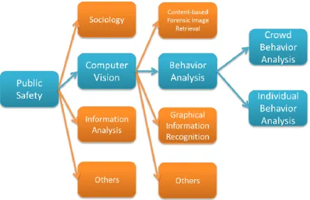
Computer Vision related researches for crowd analysis can be further categorized into application fields such as Content-based Image Retrieval (CBIR), Graphical Information Recognition (GIR) and Human Behaviour Analysis (HBA).
CBIR aims to search relative images with similar features from database according to the semantic and context of the image. It has higher requirements on retrieval speed and efficiency than conventional image retrieval that relies on pixel level operations such as histogram, moments and color set. In the last decade, some CBIR techniques attempt to utilize the semantic information extracted from an image including geometry and structure, 3D segmentation, and object recognition for various applications. Due to the nature of scientific rigorous, forensic image retrieval is a crucial tool for modern policing. Lee et al. (2012) has investigated the Tattoo Image Retrieval techniques that can be used by investigators as a viable way for suspect and victim identification.
GIR is also widely implemented in safety and security applications. Successful applications include fingerprint, vehicle registration plate, and shoeprint recognition technologies and systems. For example, shoeprints are capable of providing crucial evidence on suspect identification in forensic analysis. In most cases, shoeprint is a unique pattern similar to fingerprint. Even for shoes of same model, variant size and worn details can still be detected to distinguish different identities. Rathinavel and Arumugam (2011) proposed a novel approach on shoeprint recognition through matching partial shoeprint images with the whole image in a database. By using the proposed approach, the matched shoeprints can be used as valuable evidence in crime
3
scene investigation.
The widely installed CCTV cameras generate massive amount of live video data, these data can be utilized for predicting potential hazardous behaviours. Current main stream practical systems still reply on human operators for intervention. However, this approach has some significant disadvantages. For example, fatigue-related omission and misidentification. In order to address these issues, CV-based techniques have been developed to automate the detection tasks (Xuxin et al., 2015), (Saxena et al., 2008), (SangHyun and HangBong, 2014). These approaches have explicit advantages. However,
the challenge is still prominent since the definition of normal and abnormal behaviours is often implicit and ambiguous in real world. Therefore, how to achieve a high detection accuracy is the problem to be addressed. Figure 1-1 illustrates the field relations of this research.
Figure 1-1. Research field hierarchy, blocks in blue color represents the covered fields.
HBA can be divided into individual behaviour analysis and crowd behaviour analysis. Due to the different nature of these two types, approaches are significantly different while addressing these issues. For individual behaviour analysis, the fundamental concept is to detect and verify the actual behaviour of an individual such as waving hand, walking and running. In this approach, the target individual is firstly separated from others; then defined features are extracted from the individual. The modeled feature patterns will either be used for training the behaviour templates or
4
classifiers, or directly used for behaviour recognition. On the contrary, for crowd behaviour analysis, individuals are often treated as a whole. For example, pedestrians of close vicinity are considered as a single entity, which is segmented from the scene; then patterns or eigenvalues are extracted from this swarm. These eigenvalues are analyzed to decide which dominant behavioural type this crowd entity belongs to. An example of individual and crowd behaviour analysis is illustrated in Figure 1-2. Figure 1-2(a) is the result of using the proposed approach in the research of Lazebnik et al., (2012). In this approach, a statistical model called Bag of Word (BoW) is utilized to classify the extracted texture patch (Sivic, 2009). To be specific, the labeled image patches are firstly used to train the semantic BoW model, once the model is trained, behaviours in new images will be classified according to the texture type’s statistical distribution. In Figure 1-2(a), different poses of the figure-skater such as Camel Spin and Sit Spin are detected. Figure 1-2(b) illustrates the behaviour of a crowd of people (Ernesto et al, 2006), where the image is segmented as foreground and background. The optical flow of the foreground is calculated to train a Hidden Markov Model (HMM) (Baum and Petrie, 1966). The HMM will then be able to decide if current scene contains abnormal crowd behaviours.
(a) Analysis of Individual Behaviours illustrated in (Lazebnik, Torralba et al)
(b) Analysis of Crowd Behaviours illustrated in (Ernesto, Scott et al, 2006)
5
1.3 Key Challenges for Online Crowd Behaviour Analysis
Due to the unique patterns and factors affecting human crowds, the challenges for crowd behaviour analysis are strikingly different from individual behaviour analysis. As illustrated in Figure 1-3, three main phases must be implemented to obtain the final result for online crowd analysis. In the first phase, raw video data is obtained from either video camera or simulated footage. Also, some pre-processing of the raw video data is applied such as background subtraction as the preparation of the next phase. For the second phase, crowd’s low-level features are extracted from the processed video data, and further modelled into high-level semantic features. For the third phase, features are merged into descriptors to determine whether the anomaly exists in the crowd video. Various issues need to be addressed in each phase. This research managed to tackle 3 key issues in each of these three phases.
Figure 1-3. The procedure of crowd analysis
In the research of behaviour analysis in computer vision, wide-range of features and techniques are explored. The most appropriate feature/technique for the analysis of crowd behaviour is yet unknown. Therefore, the key issue needs to be solved is to find out the feature or descriptor which have the better performance on the recognition of crowd behaviours in the early phase of the program. The research concentrates on the support of the second and third phases of the analysis procedure to achieve the successful detection of abnormal crowd behaviours. This is the most crucial challenge to be tackled.
As the research continues, another key issue is observed while testing the devised technique for crowd abnormal behaviour classification and detection – the definition
6
and categorization of crowd behaviours is implicit and ambiguous. This issue greatly impacts the measurement of the proposed techniques’ performance. Therefore, it needs to be addressed to support the first phase of the analysis procedure.
While training and testing the devised machine learning model for behaviour classification, another major challenge is encountered – the benchmarking video datasets for crowd behaviours are extremely limited in both quantity and quality. Therefore, the third issue is the insufficiency of the crowd video data.
1.4 Project Objectives and thesis Structure
In order to address the three major challenges encountered during the research, the main objectives are summarized as follows.
• Effective extraction of Spatio-Temporal Textures (STTs) for crowd behaviour representation. This objective aims to achieve the fast and effective extraction of texture with the most motion information to support the signature modelling process of crowd behaviour analysis.
• Devising a novel descriptor/technique to achieve the recognition and classification of abnormal behaviours with high performance. This objective aims to tackle the first challenge encountered, which is the ultimate goal of this research.
• Synthesis of crowd behaviours. A simulation technique has to be devised in order to produce crowd videos with desired elements. These elements include the designated crowd population, behaviours, video quality and etc.
Contributions of this research have been made as follows.
1) In the data obtaining phase, an innovative approach is devised to simulate various types of desired crowd behaviours. This contribution attempts to tackle the insufficiency of crowd videos with desired behaviours for analysis. Because the
7
irregular visual expression and varied form of crowd behaviours. Few comprehensive benchmarking datasets existed with all desired behavioural types. Therefore, generating crowd video using simulation algorithms become a viable and important strategy.
2) In the feature extraction phase, a STT extraction approach based on information entropy is introduced to effectively obtain texture information from the STV. The feature extraction is often the most time consumptive phase in the behaviour recognition process. This contribution attempts to obtain the STT with most motion information with the least time consumption based on the core concepts of information entropy and Gabor filtering.
3) In the behaviour recognition phase, a novel crowd behaviour descriptor based on GLCM is devised to classify abnormal behaviours such as congestion and panic dispersing of a crowd. The devised descriptor is proven to outperform classic pattern filter techniques such as TAMURA (Tamura et al., 1978).
In addition, an enhanced Social Force Model (SFM) is devised to predict the individual’s destination in the crowd. When pedestrians with two different destinations are mixed in a crowd, it is inherently difficulty to identify the belonging of each pedestrian before the crowd is separated into two clusters. Inspired by the concept of boids model, an iterative approach is devised to estimate the pedestrian’s destination through an enhanced SFM.
The structure and contents of the thesis are organized as follows:
• Chapter 2 offers a comprehensive literature review of related researches, pilot systems, and their theoretical foundations;
• Chapter 3 explores the nature of the crowd behaviours categorized by a self-defined taxonomy, which leads to the revelation of the key challenges facing modern crowd behaviour analysis approaches;
• Chapter 4 then moves on to tackle the crowd motion/behaviour representation issue by devising a texture feature extraction pipeline based on the information
8
entropy theory. The ultimate goal is to achieve the efficient acquirement of motion information from live video feeds;
• Chapter 5 of the thesis defines a novel descriptor based on the Grey Level Co-occurrence Matrix (GLCM) for aiding the abnormal behaviour recognition and classification;
• Chapter 6 introduces a crowd synthesis model that integrates both long-term and short-term behaviour generating mechanisms;
• In Chapter 7, experiments and evaluations are conducted on the proposed approaches of texture extraction, crowd behaviour recognition and behaviour synthesis;
9
Chapter 2. Literature Review
In this chapter, the relative knowledges of image and video features are reviewed. Furthermore, techniques for behaviour recognition using video data are introduced. The crowd behaviour synthesis/simulation approaches are reviewed in this chapter as well.
10
2.1 Image Feature Engineering
Video features are utilized as the primary elements to model and construct pattern detectors in this research. Since video (frame) features are usually modelled in the same manners as image features, it is useful to introduce the conventional image features first which are frequently exploited in computer vision studies.
As illustrated in Figure 2-1, conventional image features consist of four basic types, which are color-based, texture-based, shape-based and spatial-relation features respectively. Color-based feature and Texture-based feature are global-scale features, which describe the object’s surface pattern in the image. Different from color-based feature, texture-based feature is often not based on single-pixel values, and could only be described by a region of neighboring pixels. Shape-based features can be further categorized into contour features and regional features. Contour features describe the boundary of a target, and regional features describe detailed information filling in an area. Spatial-relation describes the spatial or orientation relations between multiple segmented regions in an image. These relations are of adjacent, occlusion, containing etc. Spatial-relations contain relative relation and absolute relation information. The former emphasizes on the relative relations between image regions, such as up and left; while the latter focuses on the distance and angle between them.
11
2.1.1 Colour-based features
Color-based features are global-scale features, which are often single-pixel-based. Since color-based features are insensitive to the change of target’s orientation and size, they do not show good performance on capturing the local patterns. When the size of image database is too large, image indexing using color-based features will generate unwanted effects.
The Color Histogram is the most frequently used feature, it describes the global distribution of color values in the image. With advantages of rotation/translation/scaling irrelevancy, this feature can be used to describe images which are difficult to be segmented (Novak and Shafer, 1992). Since it does not include the local distribution and spatial information of colors, it is not capable of describing a specified object inside the image. Both Red-Green-Blue (RGB) and Hue-Saturation-Value (HSV) color maps are often used to quantify color histogram. The easiest approach to achieve image matching using color histogram is the Histogram Intersection. Assuming 𝑀(𝑖) and
𝑁(𝑖), which are two extracted color histograms with 𝑘 bins, where 𝑖 = 1,2, … , 𝑘. The distance of intersection 𝐷 can be represented in Equation 2-1. The smaller 𝐷 implies the higher similarity of two images.
𝐷(𝑀, 𝑁) = ∑ 𝑀𝐼𝑁(𝑀(𝑖), 𝑁(𝑖))
𝑘 𝑖=1
2-1 The Color Set is an approximation of color histogram. In order to model this feature, the color map is transformed into HSV. The transformed image is segmented and indexed with quantified color components. These color components are then transformed into a binary indexing set. Compared to color histogram, the color set feature contains spatial relation between segments. Furthermore, since the indexing set is of binary value, binary tree can be modelled to improve the indexing speed, which is beneficial in the case of large-scale image set.
In order to avoid the high dimensional vectors during the vectorization process, the feature of Color Moments is proposed in the research of Hui et al, (2002). An image is described using the Mean 𝜇, Variance 𝜎 and Skewness 𝑠 of three vectors in color map, which can be expressed in the following Equation 2-2, 2-3 and 2-4.
12 𝜇𝑖 = 1 𝑁∑ 𝑃𝑖,𝑗 𝑁 𝑗=1 2-2 𝜎𝑖 = (1 𝑁∑ (𝑃𝑖,𝑗− 𝜇𝑖) 2 𝑁 𝑗=1 ) 1 2 2-3 𝑠𝑖 = (1 𝑁∑ (𝑃𝑖,𝑗− 𝜇𝑖) 3 𝑁 𝑗=1 ) 1 3 2-4
Where 𝑃𝑖,𝑗 indicates the 𝑖th color-component of 𝑗th pixel, and 𝑁 is the number of pixels in the image. The moments of any components 𝑌, 𝑈, 𝑉 in color map will derive a 9-dimensional histogram vector as follow Equation 2-5. The advantage of color moment is the low dimension feature. This feature is mainly utilized for decreasing the indexing range in practice.
𝐹𝑐𝑜𝑙𝑜𝑟 = [𝜇𝑌, 𝜎𝑌, 𝑠𝑌, 𝜇𝑈, 𝜎𝑈, 𝑠𝑈, 𝜇𝑉, 𝜎𝑉, 𝑠𝑉] 2-5 The Color Coherence Vector (Greg et al, 1996) is another attempt to overcome the disadvantage of lacking spatial distribution of color histogram and color moment. By using a threshold, pixels in each color bin are divided into two clusters. If the size of coherence pixels is larger than threshold, these pixels are considered as converged, otherwise as non-converged. Assuming 𝛼𝑖 and 𝛽𝑖 are the number of converged and non-converged pixels in 𝑖th bin, the obtained color coherence vector would be < 𝛼1+
𝛽1, 𝛼2+ 𝛽2, … 𝛼𝑁+ 𝛽𝑁 >.
2.1.2 Texture-based Features
The texture-based features are global-scale features as well. It describes the surface pattern of a target in the image. The calculation of texture-based features often involves various pixels in certain regions. Most texture-based features are rotation irrelevant, and are resistance to noise, due to their statistical nature. A common disadvantage of texture-based features is the calculating results may vary significantly when the resolution changes. Also, the changing lighting condition will misguide the successful extraction of texture features. The texture-based features can be classified as Statistical, Geometrical, and Structural based.
13
The Grey Level Co-occurrence Matrix (GLCM) is a typical statistical feature (Haralick et al, 1973). Relationships between neighboring pixels’ Grey-scale values are used to build a co-occurrence matrix, and then key features such as Energy, Homogeneity, Entropy and Correlation are modelled from GLCM. Patterns of GLCM are exploited in the following chapter of this research as well. Another statistical approach is to extract the width and orientation of texture by calculating the energy spectrum function of an image.
Histogram of Gradient (HOG) is another widely implemented statistical feature (Dalal and Triggs, 2005). It is modelled by calculating the gradient orientation’s histogram of local image. HOG feature is frequently used in pedestrian detection with Support Vector Machine (SVM) (Cortes and Vapnik, 1995), since its high performance on describing the shape of object. Its extraction process is illustrated in Figure 2-2. In the process, image is transformed into Grey color map and divided into cells. For each cell the oriented gradients histogram with 𝑘 bins are calculated and derived into a 𝑘
dimensional vector. By using a sliding window with 𝑛 cells, the HOG of this window will be normalized as a 𝑘𝑛-dimensional descriptor. Similar statistical features include LBP (Ojala et al., 2002), Haar (Viola and Jones, 2001) and SIFT (Lowe, 1999).
Figure 2-2. Extraction process of HOG feature
The geometrical feature is based on the assumption that complicated textures could be composed with fundamental texture elements in a certain pattern. A typical geometrical feature is the Voronoi Checkboard Pathology (Ghosh and Mallett, 1994). Another approach is using parameters of image’s structural model as the texture feature.
14
The conventional approach of feature modelling is Conditional Random Fields (CRF) (He et al., 2004), Markov Random Field (MRF) (Sean, 1996), and Gibbs Random Field (Koralov and Sinai, 2012).
In the research of Mikel et al. (2011), a so-called HOG3D descriptor is devised, which is modelled with the HOG feature in spatial-temporal scale. The HOG3D is used for the local behavioural matching to address the problem of detecting rare behaviours in a large dataset.
2.1.3 Shape-based features
Shape-based features can be divided into contour and regional features. Contour features are often extracted using boundary characteristic detection algorithms. The Hough Transform is a conventional line boundary detection approach (Richard and Peter, 1972). The process of Hough transform is illustrated in following figure. In the process, edge points in the image are firstly extracted with the Canny edge detector. Next, a table of 𝜃 and 𝑟 is modelled for each point. By transforming to the polar coordinates, the intersection of curves indicates the 𝜃𝑥 and 𝑟𝑥 of possible boundary line.
Figure 2-3. Hough Transform Boundary Detection
The Fourier Shape Descriptor is another type of contour feature (Wilhelm and Mark, 2013). Exploiting the closure and periodicity, the Fourier transform of the boundary describes the shape of object. The curvature function and centroid distance are derived from the transform as descriptors.
15
representation and matching of shapes. However, the extraction of shape factors is based on the image segmentation. The accuracy of segmentation greatly affects the performance of shape factors.
The image indexing or understanding based on shape-based features share some common problems. 1) Lacking of matured mathematical model. 2) Low adaptiveness on disformed objects. 3) Mismatching between shape-based features and human subjective observation.
2.1.4 Spatial-relation Features
As above stated, the spatial-relation feature represents the spatial and directional relations between objects in the image, such as adjacent, occlusion and containing. The exploitation of spatial-relation features can improve the performance of content recognition. However, these features are sensitive to the rotation and scale-changing of the image. In practice, it is not sufficient to express the information using only the spatial-relation feature. Other features should be integrated.
In order to extract the spatial-relation features, one approach is to segment the image into regions, then extract features and create index (Barbara and Christian, 2012). Another approach is to divide the image into unified patches (Vikas et al., 2011).
2.2. Video Features
Different from features obtained from static image, video-based features often involve temporal information. By analyzing the temporal and spatial relations among multiple or consecutive frames, features can be more accurate in revealing the nature of footages. Since each video is composed of various length of frames (somewhat equivalent to static images), conventional image features are still utilized to help the modelling of visual patterns. Unlike low-level features, video-based features usually contain high-level “event” information such as semantic expression. Therefore, video-based features exhibit higher efficiency when utilized in the research of behaviour
16
understanding and recognition.
As illustrated in Figure 2-4, video-based features could be classified into flow-based features and spatial-temporal features. Because the main objective of this research is to analyze the behaviour of a crowd, a social-psychological related feature Social Force (SF) is adopted into this category as well.
Figure 2-4. Taxonomy of Video Based Features
2.2.1. Flow-based features
The most frequently utilized flow-based feature is Optical Flow. Optical flow represents the instant motion of object between two consecutive video frames (Lucas and Kanade, 1981). It is often expressed as a 2-dimensional motion vector, which incorporates the velocity along x and y directions. Due to its motion information, the optical flow is widely used as a video feature in the research of behaviour recognition, motion-based segmentation, global motion compensation and video compression.
The modelling of optical flow is based on three assumptions. 1) Brightness Consistency, where magnitudes of brightness among two consecutive frames remain constant; 2) Temporal Consistency, that the time difference between two consecutive frames should be small enough to ensure the motion consistency; 3) and, Spatial Consistency, indicating that most neighboring pixels should have the identical motion. Under ideal situation, supposing a hand gesture is captured by the camera. The spatial position of this hand is moving from one place of the first frame to another place of the next frame. At the same time, brightness magnitude of this hand remains
17
unchanged, which could be expressed as Equation 2-6.
𝑓(𝑥, 𝑦, 𝑡) = 𝑓(𝑥 + 𝑑𝑥, 𝑦 + 𝑑𝑦, 𝑡 + 𝑑𝑡) 2-6
Where 𝑓 is the brightness, 𝑑𝑥 and 𝑑𝑦 are the spatial shifting, 𝑑𝑡 is the time difference between two frames. According to the Taylor expansion, 𝑓(𝑥, 𝑦, 𝑡) could be removed and obtained Equation 2-7.
𝑓𝑥𝑑𝑥 + 𝑓𝑦𝑑𝑦 + 𝑓𝑡𝑑𝑡 = 0 2-7
By dividing 𝑑𝑡 on both sides we obtained Equation 2-8.
𝑓𝑥𝑑𝑥 𝑑𝑡 + 𝑓𝑦
𝑑𝑦
𝑑𝑡+ 𝑓𝑡 = 0 → 𝑓𝑥𝑢 + 𝑓𝑦𝑣 + 𝑓𝑡= 0 2-8
Where 𝑢 and 𝑣 are optical flows along 𝑥 and 𝑦 directions. The main stream approaches to solve 𝑢 and 𝑣 are the Horn-Schunk (HS) method and the Lucas-Kanade (LK) method.
a) Horn-Schunk method
The HS method (Horn and Schunck, 1981) adapts an additional smoothness constraint to address the solution of 𝑢 and 𝑣 . This constraint assumes the velocity difference between pixel and its neighbors is limited. Therefore, acquiring 𝑢 and 𝑣
becomes an optimization problem of the objective function.
𝑚𝑖𝑛 ∬(𝑓𝑥𝑢 + 𝑓𝑦𝑣 + 𝑓𝑡)2+ 𝜆(𝑢𝑥2+ 𝑢𝑦2+ 𝑣𝑥2+ 𝑣𝑦2)𝑑𝑥𝑑𝑦 2-9 By traversing every pixel on the image, find a combination of 𝑢 and 𝑣 to minimize the objective function. Its first term is the brightness constraint, and the second term is the smoothness constraint. By applying partial derivate, two functions can be obtained, which could be used to get 𝑢 and 𝑣.
{(𝑓𝑥𝑢 + 𝑓𝑦𝑣 + 𝑓𝑡)𝑓𝑥+ 𝜆(∆
2𝑢) = 0
(𝑓𝑥𝑢 + 𝑓𝑦𝑣 + 𝑓𝑡)𝑓𝑦 + 𝜆(∆2𝑣) = 0
2-10
b) Lucas-Kanade method
The LK method made an additional assumption that the local pixels have identical optical flow (Lucas and Kanade, 1981). According to the brightness constraint equation, we can obtain the following Equations 2-11.
18 𝑓𝑥1𝑢+𝑓𝑦1𝑣=−𝑓𝑡 𝑓𝑥2𝑢+𝑓𝑦2𝑣=−𝑓𝑡 … 𝑓𝑥𝑛𝑢+𝑓𝑦𝑛𝑣=−𝑓𝑡 2-11
Where 1,2 … 𝑛 are pixels in the local window. The equations above could be represented as 𝐴𝑈 = 𝑏 . By pre-multiplying the transposition of 𝐴 , we obtain
𝐴𝑇𝐴𝑈 = 𝐴𝑇𝑏. If the inversed matrix of 𝐴𝑇𝐴 exists, the LK optical flow will be 𝑈 =
(𝐴𝑇𝐴)−1𝐴𝑇𝑏.
c) Properties of optical flow
The optical flow exhibits high efficiency on the research of behaviour recognition. After further investigation, researcher reveal following patterns of optical flow (Beauchemin and Barron, 1995): 1) The reason of its effectiveness on behaviour recognition is the invariance to the image’s appearance, rather than its capability of capturing the motion information; 2) Accuracy of edges and minor spatial shifting that leads to distinctive behavioural patterns; and, 3) Object detection tasks can be achieved using optical flow information alone even on moving camera without contextual or environmental information.
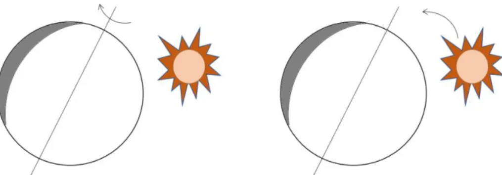
The major disadvantage of optical flow is that it may not work without the constraints as stated before. For instance, it may not correctly abstract the real motion caused by objects due to illumination conditions. As illustrated in Figure 2-5, if the target object’s texture is uniformed and light source is static, the rotation of spherical object will not generate interpretable optical flow. On the other hand, when the light source is moving and object remain static, the optical flow might be generated by reflections and shadows. This result implies the optical flow is sensitive to illumination conditions. When the motion velocity is too high, conventional optical flow method may be falling too. Unfortunately, objects caught in a video of high velocity are commonplace.
19
Figure 2-5. (a) Moving but without optical flow. (b) Static but with optical flow.
Various improved flow-based features are proposed by researchers to improve the robustness of optical flow, which includes Streak Flow (Mehran et al., 2010), Tracklet (Seung and Kuk, 2014), and Particle Flow (Ali and Shah, 2007).
However, in general, sparser optical flow are still confronted by aperture problems, and the denser optical flow has the disadvantage of high computational time consumption, which made it inappropriate for real-time processing.
2.2.2 Spatial-Temporal Features
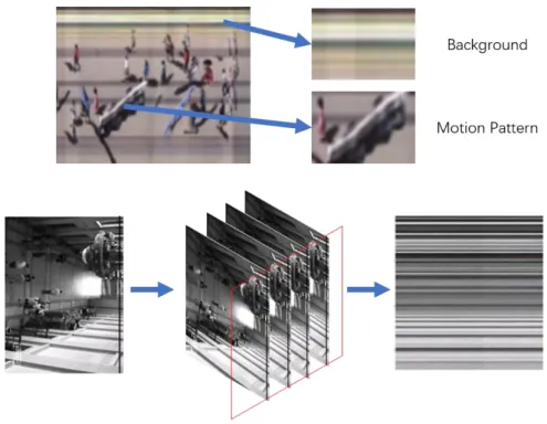
Flow-based features can be utilized to detect dominant events, however for the unstructured high-density crowd scenes, even a fine-grain representation such as optical flow would not provide enough motion information for processing. Thus Spatial-Temporal features are used to detect abnormality to compensate the deficiencies. The related methods generally consider the motion as a whole, and characterize its spatial-temporal distributions based on local 2D pixel patches and 3D voxel (volumetric-pixel) cubic. Spatial-temporal features have sound performance in motion understanding due to their strong descriptive power (Jing and Zhijie, 2016), and unlike flow-based features,
the temporal information is preserved. a) Spatial-Temporal Volume
The Spatial-Temporal Volume (STV) is a Spatial-Temporal model introduced by Adelson and Bergen (1985). The process of modelling the STV is illustrated in Figure 2-6. In the first step, a set of consecutive video frames is obtained from the dataset or real-time video stream. These frames will be stacked up along time sequence. The selection of the frame’s indices is based on the actual video length, or the requirement
20
for the system. Each frame could be of Grey scale or RGB format. The size of selected data can be the entire frame or a portion of it. Once these frames are selected, they will be stacked together to generate a cube-shaped structure. According to the selection of width, height and number of frames, the size of this cube may be varied.
The STV block can be viewed as a stretching of 2D pixels into 3D voxels and filling the entire 3D space. Therefore, the STV holds certain advantages comparing to the two-dimensional patterns on behaviour analysis. For example, the STV block contains temporal information such as trajectories of pedestrians.
Figure 2-6. The STV modelling and STT extraction
STV is widely utilized in action recognition, for example, Bolles et al. (1987) introduced a technique for the recovery of the geometric and structure information from a static scene using the STV. Kühne et al. (2001) exploits STV to achieve 3D scene segmentation. The two latest deep learning frameworks - the 3D convolution network with STV data (Bo et al., 2012) and the two-steam network with optical flows – have
also been based on STV features. b) Spatial-Temporal Texture
As stated in previous section, flow-based features have sound performance when the motion velocity is low. In order to extract the temporal information in a more robust way, the detailed information can be extracted from the STV.
The textures within STV is named Spatial-Temporal Texture (STT), which could be used to extract patterns for modeling spatial and temporal signatures for behaviour
21
analysis. According to the requirements for different analyzing approaches, STT can be extracted in either 2D format or volume-based. The process of 2D STT extraction is illustrated in Figure 2-6. A STV block is sliced along horizontal or vertical directions. Each slice with one pixel in thickness is the obtained 2D STT. One possible approach to achieve the volume-based extraction is to implement background subtraction for each frame, and then keep the foregrounds pixels of interested objects.
In practice, researchers attempted to detect the single person’s gestures such as cuts, wipes and waving hands using STT patterns (Ngo et al., 1999). The approach first extract STT that is convolved with a derivative Gaussian filter. The convolved result is further processed with the Gabor decomposition where the real components of multiple spatial-frequency channel envelopes are obtained before being modelled into texture feature vectors. Finally, a Markov energy-based image segmentation approach is applied on these vectors to determine the matched gesture type.
2.2.3 Semantic Features
By further exploring the low-level features such as optical flow, semantic features can be modelled by incorporating “meaningful” high-level information. The most widely adapted semantic features in the research of crowd behaviour is the so-called “Social Force” for its sociology nature of describing agents behaviour in a crowd.
Figure 2-7. Acceleration, Repulsive and Obstacle Avoidance Forces in SFM
22
assumes that an agent in the crowd is always influenced by several forces derived from planned destination, neighbors in vicinity, and obstacles ahead and around. These forces determine the instant motion of a target agent. SFM can be obtained using Equation 2-12.
𝑠𝑓𝑖= 𝑓𝑑+ ∑ 𝑓𝑗𝑖 𝑗≠𝑖
+ ∑ 𝑓𝑜𝑘𝑖 2-12
Where 𝑠𝑓𝑖 indicates the final social force applied to pedestrian 𝑖. 𝑓𝑑 indicates the acceleration force, which derives from the agent’s desire of heading the destination with constant magnitude. 𝑓𝑗𝑖 indicates the social attraction and repulsive forces, which derives to avoid collision between agent 𝑖 and 𝑗 . 𝑓𝑜𝑘𝑖 indicates the obstacle avoidance force between obstacle 𝑘 and pedestrian 𝑖.
𝑓𝑗𝑖 can be expressed as Equation 2-13, where 𝐴𝑖 and 𝐵𝑖 are constants to control the magnitude of 𝑓𝑗𝑖 . 𝑟𝑖𝑗 is the summation of agent 𝑖 and 𝑗 ’s radius. 𝑑𝑖𝑗 is the distance between 𝑖 and 𝑗. 𝑛𝑖𝑗 is the normalized vector to control 𝑓𝑗𝑖’s direction. The exponential function guarantees the fast magnification of 𝑓𝑗𝑖 when two agents are getting too close. On the contrary, if 𝑑𝑖𝑗 is large, magnitude of 𝑓𝑗𝑖 will have a fast reduction. Similarly, the obstacle avoidance force 𝑓𝑜𝑖 is derived when agent moves to obstacles such as walls.
𝑓𝑗𝑖 = 𝐴𝑖𝑒(𝑟𝑖𝑗−𝑑𝑖𝑗)/𝐵𝑖𝑛𝑖𝑗 2-13
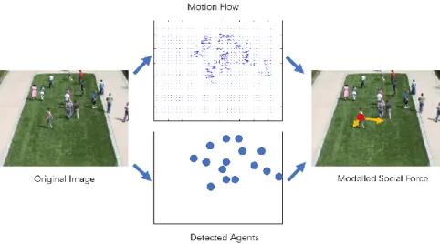
Process of modelling social force is illustrated in Figure 2-8. The map of motion flow/optical flow is extracted from the original image. Pedestrians’ positions are located with pedestrian detector in parallel process. Then 𝑓𝑑, 𝑓𝑗𝑖 and 𝑓𝑜𝑘𝑖 can be modelled using the introduced equations.
23
Figure 2-8. Process of modelling Social Force
The modelled social force is used as features in the training and testing processes of the machine learning model such as Support Vector Machine (SVM) to classify the pedestrian’s behaviours (Lei Q. et al., 2012). The research of Mehran (2009) also exploited social force with BoW statistical model to detect the abnormal frames in the video.
2.3 Techniques for Behaviour Recognition
The techniques for behaviour recognition can be divided into two main branches, conventional approaches and deep learning-base ones. The conventional approaches use selected video features to train the machine learning model and understand the behaviour types. On the opposite, the core concept of deep learning is to feed large number of video data to the convolution neural network, so that the network can extract most efficient features in an unsupervised manner. Generally, machine learning has better performance than conventional approaches in recent years, but some conventional approaches such as improved Dense Trajectories (iDT) still have significant efficiency on behaviour recognition. Section 2.3.1 introduces the general procedure of conventional approach. Section 2.3.2 provides the detail of the state-of-the-art conventional behaviour recognition approach, the dense trajectories. Section
24
2.3.3 gives introduction to the deep learning approaches.
2.3.1 General Procedure of Conventional approach
Behaviour Recognition is essentially a classification problem in computer vision. The general procedure of conventional approach consists of feature extraction, feature fusion and feature classification as illustrated in Figure 2-9.
Figure 2-9. General Procedure of Conventional Approach
a) Feature Extraction
In order to extract features, either the 2-dimensional spatial information from image frame or the temporal information from video sequence are utilized. According to the modelling methods, the conventional feature extraction can be categorized as global and local approaches. The global approaches consider the entire video frame as an entity, extracting global feature with a top-down strategy of feature point detection, neighboring feature calculation and feature integration. Global approaches are insensitive to local occlusion and noise. On the contrary, its performance is heavily correlated to the number of feature points. The Local approaches concentrate on a segment of the video sequence, extracting feature with a bottom-up strategy of human detection, background tracking and region of interest encoding. The advantage of local approaches is the sufficiency of encoding information. The disadvantages are the reliance on the accuracy of human detection and sensitive to the noise and occlusion. The feature points are most widely exploited feature in the conventional behaviour recognition. Some state-of-the-art features are Space-Time Interest Points (STIP) proposed by Ivan (2005), Cuboid proposed by Rabaud et al. (2005), Motion Energy Image (MEI) & Motion History Image (MHI) proposed by Bobick and Davis (2001) and HOG & HOF proposed by Ivan et al. (2008).
25
b) Feature Fusion
The contour, boundary and motion features of human aren’t compatible to each other. Since they usually have different dimensions and data structures, which cannot be utilized directly before being modelled. In order to acquire features with higher adaptiveness and efficiency, the feature fusion process is necessary. Furthermore, the feature fusion/encoding can remove the redundant information and enhance the accuracy of behaviour understanding. Main stream approaches of feature fusion include the Bag of Feature (BoF) and Fisher Vector. The extracted features such as texture, contour and optical flow are defined as low-level features. The fused low-level features are defined as mid-level features, and the classified features are defined as high-level semantic features in this research.
⚫ Bag of Feature
Bag of Feature (BoF) is also named Bag of visual Word (BoW) first proposed by Lazebnik et al. (2006), which is originated from the Bag of Words in the linguistics. Similar to linguistics, the key features could be extracted from the image data to model the visual word. By using the k-means classifier to cluster the features, similar features are considered as one class. The center of the cluster is the visual word. The statistic of each visual word is the codebook whose size is the number of classes. Due to the differences between the text and visual features, the strategy of local feature sampling, size of codebook, weight calculation of visual word and modelling of codebook are still major challenges to be tackled.
The construction of BoW follows the order of extracting low-level features extraction and clustering, codebook establishment based on formulated clusters. And finally, classifier training using the Visual Words (clusters) from the codebook.
⚫ Fisher Vector
Fisher Vector is another fusion technique proposed by Florent and Christopher (2007). Similar to BOW, it is also capable of achieve the normalization of feature matrices with different length. For example, the video features from videos with different length will generate feature matrices with different size. Before sending to the
26
neural network for classification, the feature matrices need to be processed into uniformed size. The BoW approach ignores the spatial relationship between the low-level features, and the computational complexity is high. Furthermore, the BoW needs to be retrained when a new class is inserted. The Fisher Vector addressed these issues by using Expectation Maximization to train the SIFT descriptor with a wholesale of weighting, mean and covariance matrices and spatial distribution outputs.
2.3.2 The State-of-the-art Conventional approach
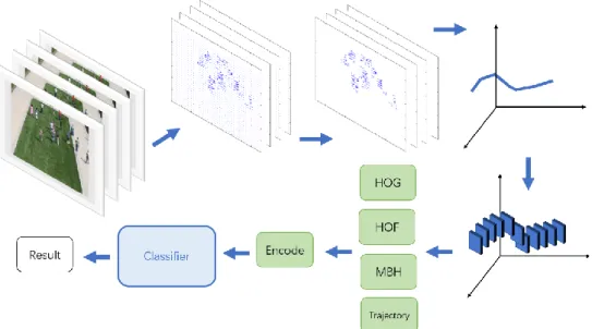
iDT has the best performance of behaviour recognition among conventional approaches, which is proposed by Wang and Schmid (2013). In this section, iDT’s original version Dense Trajectories (DT) is introduced as an example to explain the details (Wang et al., 2013). The procedure is illustrated in Figure 2-10. According to the general procedure of DT, the feature points are firstly sampled with a filtering process. Next, the trajectories are extracted for each sample points. Then the STV around each trajectory is modelled for the calculation of HOG, Histogram of Optical Flow (HOF) and Motion Boundary Histogram (MBH). Finally, the normalized and encoded features are classified for the analyzing result.
Figure 2-10. Procedure of DT behaviour recognition
a) Dense Feature Points Sampling
27
optical flow. Multiple spatial scales ensure the features to have a full coverage on all spatial scales. Next, feature points are tracked at the temporal scale. However, tracking is invalid with feature points of motionless background. Therefore, a threshold is adapted to remove feature points with low motion. The threshold 𝑇 could be expressed as Equation 2-14.
𝑇 = 0.001 × 𝑚𝑎𝑥𝑖∈𝐼𝑚𝑖𝑛 (𝜆1𝑖, 𝜆𝑖2) 2-14
Where (𝜆𝑖1, 𝜆𝑖2) are the modelled optical flow feature of pixel 𝑖 in image 𝐼. 𝜆1𝑖
indicates the flow magnitude along the horizontal direction, and 𝜆𝑖2 indicates the magnitude along the vertical direction. The experiment indicates 0.001 is the most appropriate value in the filtering process.
b) Trajectory Descriptor
Assume the spatial position of the extracted feature point is 𝑃𝑡 = (𝑥𝑡, 𝑦𝑡), its spatial position in the next frame could be expressed as Equation 2-15.
𝑃𝑡+1= (𝑥𝑡+1, 𝑦𝑡+1) = (𝑥𝑡, 𝑦𝑡) + (𝑀 ∗ 𝑤𝑡)|𝑥𝑡,𝑦𝑡 2-15 Where 𝑤𝑡 = (𝑢𝑡, 𝑣𝑡) is the dense optical flow obtained from 𝐼𝑡 and 𝐼𝑡+1. 𝑀 is an average filter. The trajectory of a feature point during consecutive 𝐿 frames could be expressed as (𝑃𝑡, 𝑃𝑡+1, … , 𝑃𝑡+𝐿). Because of the shifting of feature point, long-term tracking is often unreliable. Therefore, sampling process is conducted for each 𝐿
frames repeatedly.
Furthermore, obtained trajectory could be used to model the trajectory shape descriptor. Assume a trajectory with length 𝐿 is expressed as (∆𝑃𝑡, … , ∆𝑃𝑡+𝐿−1) , where ∆𝑃𝑡 = (𝑃𝑡+1− 𝑃𝑡) = (𝑥𝑡+1− 𝑥𝑡, 𝑦𝑡+1− 𝑦𝑡). The descriptor could be obtained by regularizing with Equation 2-16.
𝐷 =(∆𝑃𝑡, … , ∆𝑃𝑡+𝐿−1) ∑𝑡+𝐿−1𝑗=𝑡 ||∆𝑃𝑗||
2-16
c) Motion and Structure Descriptors
The DT and iDT further exploit features including HOF, HOG and MBH to represent the motion. Along the obtained trajectory with length 𝐿, areas with size of
28
𝑁 × 𝑁 pixels are modelled as a STV. Next, the STV is divided by a 𝑛𝜎 × 𝑛𝜎× 𝑛𝜏
grid, where 𝑛𝜎 is the grid’s size along spatial space, and 𝑛𝜏 is the grid’s size along temporal space. In DT and iDT, 𝑁 = 32, 𝑛𝜎 = 2, 𝑛𝜏 = 3. Next, HOG, HOF and MBH are extracted from these volume blocks.
⚫ HOG – HOG is the histogram of gradient of the Grey scale image. The bin number is set as 8, thus the dimension of HOG is 2 ∗ 2 ∗ 3 ∗ 8 = 96.
⚫ HOF – HOF is the histogram of optical flow including the magnitude and direction information. The number of bins is set as 8 + 1, where 8 bins are identical to HOG, the extra bin is used for the statistic value of the number of pixels which is than a threshold. The dimension of HOF is 2 ∗ 2 ∗ 3 ∗ 9 = 108. ⚫ MBH – MBH is the HOG feature on the optical flow map. The MBH is along
two directions 𝑥 and 𝑦, thus its dimension is 2 ∗ 96 = 192. These features are normalized with the L2-norm.
d) Feature Encoding and Classification
For each video sequence, various trajectories could be extracted with a set of features. DT uses BOF (Feifei and Perona, 2005) to encode these features. The code book is trained with 100000 feature sets, and its size is set to 4000. Once encoded, features are classified by SVM with the RBF kernel, the classification result indicates the recognized behaviour.
The framework of iDT is identical to DT, the improvement concentrates on the optimization of optical flow and feature encoding. As the result, the efficiency is significantly improved. The accuracy increases from 84.5% to 91.2% on UCF50 set (Kishore and Mubarak, 2012), and from 46.6% to 57.2% on HMDB51 set (Kuehne et al. 2011).
2.3.3 Behaviour Recognition using Deep Learning Framework
As the fast development of deep learning, Convolutional Neural Network (CNN) becomes the main stream classification approach in computer vision. The miss-rate of ResNet-152 is 3.5%, which outperforms the 5.1% miss-rate of human vision. In order
29
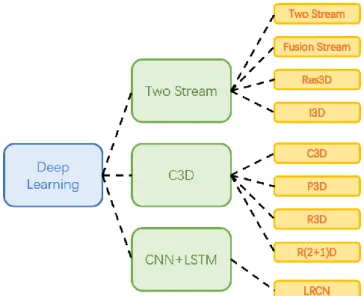
to achieve the fusion of spatial and temporal features, three main branches are proposed by researchers, which are Two Stream (Karen and Andrew, 2014), Convolution 3D (Du
et al., 2015) and CNN-Long Short-Term Memory (CNN-LSTM) (Tara et al., 2015). The structure of deep learning approaches on computer vison could be illustrated as Figure 2-11.
Figure 2-11. Taxonomy of Deep Learning Approaches
The general procedure of Deep Learning consists of 6 phases, which are data pre-processing, network building, definition of classification function and Loss function, definition of optimizer, training, validating and testing process. The procedure is illustrated as Figure 2-12.
Figure 2-12. General procedure of deep learning
a) Data Pre-processing
In this phase, the data set is evenly divided as training set, validating set and testing set with random distribution. Since the deep learning is a resource consuming task, the parallel computing is required. The parallel computing includes data parallelism and model parallelism. The data parallelism is to process a mini batch of data on multiple devices, in order to achieve the parallelism of gradient computing. The model parallelism is to process different models of a neural network on different devices, in