A plane of high velocity galaxies across the Local Group

A Plane of High Velocity Galaxies Across the Local Group

Indranil Banik

∗

, Hongsheng Zhao

1_{Scottish Universities Physics Alliance, University of St Andrews, North Haugh, St Andrews, Fife, KY16 9SS, UK}

8 October 2017

ABSTRACT

We recently showed that several Local Group (LG) galaxies have much higher radial velocities (RVs) than predicted by a 3D dynamical model of the standard cosmological paradigm. Here, we show that 6 of these 7 galaxies define a thin plane with root mean square thickness of only 101 kpc despite a widest extent of nearly 3 Mpc, much larger than the conventional virial radius of the Milky Way (MW) or M31. This plane passes within ∼70 kpc of the MW-M31 barycentre and is oriented so the MW-M31 line is inclined by 16◦ to it.

We develop a toy model to constrain the scenario whereby a past MW-M31 flyby in Modified Newtonian Dynamics (MOND) forms tidal dwarf galaxies that settle into the recently discovered planes of satellites around the MW and M31. The scenario is viable only for a particular MW-M31 orbital plane. This roughly coincides with the plane of LG dwarfs with anomalously high RVs.

Using a restricted N-body simulation of the LG in MOND, we show how the once fast-moving MW and M31 gravitationally slingshot test particles outwards at high speeds. The most distant such particles preferentially lie within the MW-M31 orbital plane, probably because the particles ending up with the highest RVs are those flung out almost parallel to the motion of the perturber. This suggests a dynamical reason for our finding of a similar trend in the real LG, something not easily explained as a chance alignment of galaxies with an isotropic or mildly flattened distribution (probability = 0.0015).

Key words: galaxies: groups: individual: Local Group – Galaxy: kinematics and dynamics – Dark Matter – methods: numerical – methods: data analysis – cosmology: cosmological parameters

1 INTRODUCTION

The standard cosmological paradigm (ΛCDM) faces several challenges in the relatively well-observed Local Group (LG). In particular, the satellite systems of its two major galaxies −the Milky Way (MW) and Andromeda (M31)−both ex-hibit an unusual degree of anisotropy. For the MW, this has been suspected for several decades (Lynden-Bell 1976,1982), though recent observations have greatly clarified the situa-tion and its apparent tension with ΛCDM (Kroupa et al. 2005). Proper motion measurements show that most of its satellites co-rotate within a well-defined plane (Pawlowski & Kroupa 2013). Moreover, recently discovered ultra-faint satellites, globular clusters and tidal streams independently prefer a similarly oriented plane (Pawlowski et al. 2012). Although some flattening is expected in ΛCDM (e.g.Butsky et al. 2016), it remains difficult to explain the very small

∗Email:[email protected](Indranil Banik) [email protected](Hongsheng Zhao)

thickness of the MW satellite system and its coherent rota-tion (Pawlowski et al. 2015).

An analogous situation was suspected around M31 (Metz et al. 2007,2009). This has recently been confirmed byIbata et al. (2013) using the Pan-Andromeda Archaeo-logical Survey (McConnachie et al. 2009). Despite its greater distance, the detection of this highly anisotropic system is rather secure because it is almost edge-on as viewed from our perspective. A redshift gradient across it strongly sug-gests that it too is co-rotating (Ibata et al. 2013). Like the MW satellite system, it is difficult for ΛCDM to explain the observed properties of the M31 satellite system (Ibata et al. 2014).

find in cosmological simulations of the ΛCDM paradigm (Gonz´alez & Padilla 2010, Figure 8).

We recently uncovered another potential problem relat-ing to the dynamics of non-satellite LG dwarf galaxies at dis-tances of∼1−3 Mpc (Banik & Zhao 2016). This was based on a timing argument analysis of the LG (Kahn & Woltjer 1959;Einasto & Lynden-Bell 1982) extended to include test particles representing LG dwarfs. Following on from previ-ous spherically symmetric dynamical models (Sandage 1986; Pe˜narrubia et al. 2014), we constructed an axisymmetric model of the LG consistent with the almost radial MW-M31 orbit (van der Marel et al. 2012b) and the close alignment of Centaurus A with this line (Ma et al. 1998). Treating LG dwarfs as test particles in the gravitational field of these three massive moving objects, we investigated a wide range of model parameters using a full grid search. None of the models produced a good fit, even when we made reasonable allowance for inaccuracies in our model as a representation of ΛCDM based on the scatter about the Hubble flow in de-tailedN-body simulations of it (Aragon-Calvo et al. 2011). This is because several LG dwarfs have Galactocentric Ra-dial Velocities (GRVs) much higher than expected in our best-fitting model, though the opposite was rarely the case (Banik & Zhao 2016, Figure 9). We found that this should remain true even when certain factors beyond the model are included, in particular the Large Magellanic Cloud and the Great Attractor (GA).

We borrowed an algorithm described in Peebles et al. (2011) to test whether this remains the case when using a three-dimensional (3D) model of the LG. The typical mis-match between observed and predicted GRVs in the best-fitting model is actually slightly higher than in the 2D case, with a clear tendency persisting for faster outward motion than expected (Banik & Zhao 2017a, Figures 7 and 9). These results are similar to those obtained byPeebles(2017) using a similar algorithm. Despite a very different method toBanik & Zhao(2016), the conclusions remain broadly similar.

Beyond the LG, another puzzling observation in a ΛCDM context is the remarkably tight correlation between the internal accelerations within galaxies (typically inferred from their rotation curves) and the prediction of Newtonian gravity applied to the distribution of their luminous matter (e.g.Famaey & McGaugh 2012, and references therein). This ‘radial acceleration relation’ (RAR) is a generalisation of the baryonic Tully-Fisher relation (e.g.McGaugh & Schombert 2015) which only considers the flat outer part of galaxy ro-tation curves and their total baryonic masses (Equation3), whereas the RAR considers all radii with accurate data.

The RAR has recently been confirmed and further tight-ened based on near-infrared photometry taken by the Spitzer Space Telescope (Lelli et al. 2016), considering only the most reliable rotation curves (as described in its Section 3.2.2 and also inSwaters et al. 2009) and taking advantage of reduced variability in stellar mass-to-light ratios at these wavelengths (Bell & de Jong 2001;Norris et al. 2016). These improve-ments reveal that the RAR holds with very little scatter over ∼5 orders of magnitude in luminosity and a similar range of surface brightness (McGaugh et al. 2016).

In addition to disk galaxies, the RAR also seems to hold for ellipticals, whose internal forces can sometimes be measured accurately due to the presence of a thin rotation-supported gas disk (den Heijer et al. 2015). As well as these

massive ellipticals, the RAR also works well in galaxies as faint as the satellites of M31 (McGaugh & Milgrom 2013). For a recent overview of how well the RAR works in several different types of galaxy across the Hubble sequence, we refer the reader toLelli et al.(2017).

The RAR is either a fundamental consequence of nat-ural law or an emergent property of galaxies relating their baryonic and dark matter distributions. The latter approach is taken by ΛCDM, a paradigm in which a relation of this sort is expected because lower mass dark matter halos have shallower gravitational potential wells. This should make it easier for baryons to be ejected via energetic processes like supernova feedback. Still, the tightness of the observed RAR is difficult to explain in this way (Desmond 2017). Some attempts have been made to do so (e.g.Keller & Wadsley 2017), but so far these have investigated only a very small range of galaxy masses and types. In these limited circum-stances, there does seem to be a tight correlation of the sort observed. However, a closer look reveals that several other aspects of the simulations are inconsistent with observations (Milgrom 2016). For example, the rotation curve amplitudes are significantly overestimated in the central regions (Keller et al. 2016, Figure 4).

Unlike ΛCDM, Modified Newtonian Dynamics (MOND, Milgrom 1983) is predicated on the assumption that the RAR is fundamental and not due to galaxies being sur-rounded by dark matter halos. The dynamical effect of these halos is instead provided by a revised law of gravity arising from an acceleration-dependent modification to the Poisson equation of Newtonian gravity (Bekenstein & Milgrom 1984; Milgrom 2010). In spherical symmetry, the gravitational field strength g at distance r from an isolated point mass

M transitions from the usual inverse square law at short range to

g =

p GM a0

r for r

s GM

a0

(1)

Here,a₀ is a fundamental acceleration scale of nature. Empirically, a0 ≈1.2×10

−10

m/s2 to match galaxy rota-tion curves (McGaugh 2011). Remarkably, this is similar to the acceleration at which the energy density in a classical gravitational field becomes comparable to the dark energy densityuΛ =ρΛc

2

implied by the accelerating expansion of the Universe (Riess et al. 1998). Thus,

g2

8πG < uΛ ⇔ g . 2πa0 (2)

This suggests that MOND may arise from quantum gravity effects (e.g.Milgrom 1999;Pazy 2013;Verlinde 2016; Smolin 2017). Regardless of its underlying microphysical explanation, MOND can explain the Tully-Fisher relation (Tully & Fisher 1977) as a specific example of the RAR by equating the gravitational field strength given by Equation 1with the centripetal acceleration v_r2 required to maintain a circular orbit. In the low-acceleration outskirts of galaxies beyond the extent of most of their visible mass1, this predicts a flat rotation curve with amplitude

v_f = p4

GM a₀ (3)

Although this is one of the more widely known conse-quences of MOND, the theory does much more than this and more even than the RAR, its prediction in isolated systems. For the recently discovered Crater 2 satellite of the MW (Torrealba et al. 2016), it predicted the velocity dispersion to be a tiny 2.1 km/s (McGaugh 2016b), partly due to a unique effect in MOND whereby its self-gravity is weakened by the external gravitational field of the nearby MW (e.g. Banik & Zhao 2015). This was recently confirmed by observations, which are in tension with a naive application of the RAR but not a more rigorous treatment of MOND (Caldwell et al. 2017). This external field effect hardly matters for calculat-ing the rotation curve of the MW but is crucial to its escape velocity, measurements of which can be fit reasonably well in MOND (Banik & Zhao 2017b).

A crucial ingredient for the RAR is the strength of the gravitational field in the outskirts of galaxies. These are impossible to measure directly and can only be estimated from rotation curves. Gravitational lensing provides an in-dependent way to check these estimates in a statistical sense. One such attempt was the Canada-France-Hawaii Telescope Lensing Survey (Brimioulle et al. 2013). Stacked data from it shows that MOND can predict the correct amplitude of weak gravitational lensing by spiral and elliptical galaxies, using Equation1with the same value fora0as that required

to match disk galaxy rotation curves (Milgrom 2013). Thus, weak lensing and rotation curve measurements broadly agree on the strength of gravity in the outskirts of galaxies.1

As well as affecting forces within a galaxy, MOND also affects forces between them. In the LG, this implies a much stronger MW-M31 mutual attraction than ΛCDM. Com-bined with the almost radial nature of their relative motion (van der Marel et al. 2012b), this means that they must have undergone a close encounter ∼9±2 Gyr ago (Zhao et al. 2013). This could have led to the formation of a thin tidal tail which later condensed into satellite galaxies of the MW and M31, a phenomenon which seems to occur in some observed galactic interactions (Mirabel et al. 1992) and in MOND simulations of them (Tiret & Combes 2008).The formation mechanism of these tidal dwarf galaxies would lead to them lying close to a plane and co-rotating within that plane (Wetzstein et al. 2007), though a small fraction might well end up counter-rotating (Pawlowski et al. 2011). Some could even become unbound from both the MW and M31, instead flying away from the LG at high speed. This is possible once the effect of dark energy is considered as its repulsive effect rises with distance, unlike the gravitational field from a finite distribution of matter (Equation22).

A past MW-M31 interaction might also have formed the thick disk of the MW (Gilmore & Reid 1983), a structure which seems to have formed fairly rapidly from its thin disk 9±1 Gyr ago (Quillen & Garnett 2001). More recent inves-tigations suggest a fairly rapid formation timescale (Hayden et al. 2015) and an associated burst of star formation (Snaith et al. 2014, Figure 2). The disk heating which likely formed the Galactic thick disk appears to have been stronger in

1 _{Although MOND is a non-relativistic theory, all attempts to} generalise it to the relativistic case imply that the non-relativistic gravitational field determines light deflection in the same way as in General Relativity (Milgrom 2013, Section 2).

the outer parts of the MW, characteristic of a tidal effect (Banik 2014). This may be why the thick disk of the MW has a larger scale length than its thin disk (Juri´c et al. 2008; Jayaraman et al. 2013).

The high MW-M31 relative velocity around the time of their encounter (∼600 km/s,Zhao et al. 2013) suggests that they could well have flung out several LG dwarfs at high speed in what would essentially have been 3-body gravita-tional interactions (Banik & Zhao 2016). The main objective of the present contribution is to test certain aspects of this scenario. In Section 2, we extract some of its likely con-sequences based on a toy model of a past MW-M31 flyby encounter. Linking this to the observed geometry of the LG gives a constraint on the MW-M31 orbital plane. In Section 3, we use this in a more detailed MOND simulation of the LG incorporating several hundred thousand test particles affected by the gravity of the MW and M31, which undergo a close (14.17 kpc) flyby 6.59 Gyr after the Big Bang. As expected, some particles are flung out at high radial veloc-ities after passing close to the spacetime location of this event. The particles flung out to the greatest distances have orbital angular momenta aligning rather closely with that of the MW-M31 orbit (Figure8) and lie rather close to the MW-M31 orbital plane (Figure9). This is probably because such particles were ejected almost parallel to the motion of the perturbing body in order to gain the most energy from it.

In Section 4.1, we refine our previous ΛCDM model of the LG in 3D (Banik & Zhao 2017a) to help us better select LG galaxies whose kinematics suggest that they were flung out in this way. We quantify the spatial anisotropy of these galaxies in Section 5. Here, we use our MOND-based simulation to identify three further properties that we expect of these high-velocity galaxies (HVGs). In Section 6, we quantify how likely it is for a random distribution of HVGs to match these properties as well as the observed HVG system. In Section7, we discuss our analysis in light of previous works and consider some possibilities for explaining our results within MOND (Section7.1) and ΛCDM (Section 7.2). Our conclusions are given in Section8.

2 GEOMETRY OF A PAST MW-M31 FLYBY

2.1 Orientation of the M31 disk

We begin by describing how we find the angular momentum direction of the M31 diskhb_M31, where we define the unit

vectorbv≡

v

|v| for any vectorv. Based on the ellipticity of its image, we know the inclinationiof the M31 disk to the plane of our sky. The orientation of this image is described by a position angleψ, whose meaning is illustrated in Figure1. Our adopted values for these parameters are given in Table 1, the caption of which contains the relevant references.

The major axis of the M31 image corresponds to the directionM A[ ∝rbM31×hb_M31, which is orthogonal to both

the directionr_bM31 towards M31 and tobh_M31 as it must lie

ψ

North

East

Major axis MA Figure 1.This is how an external disk galaxy like M31 appears on our sky. The direction towards the centre of its image (into screen) isrbM31. Its posi-tion angleψis defined as the angle of its major axisM A[eastwards of the lo-cal North (Equation5). Its inclination ito the sky plane can be determined from the ellipticity of its image.

Variable Meaning Value

b

r_M31 Direction to M31 now (121.57◦_,−21.57◦₎ i Inclination of M31 77.5◦

disk to sky plane

ψ Position angle of M31 disk 37.7◦_±0.9◦ on sky (Figure1)

b

hM31 Internal angular momentum (238.65

◦_,−26.89◦₎ direction of M31 disk

Table 1. Observational parameters of M31 important for this work. Its sky position in Galactic co-ordinates (latitude last) is fromEvans et al.(2010). We also give its inclination (Ma 2001) and position angle (Chemin et al. 2009, Section 5.2). Combined with radial velocity measurements, this implies its disk has a par-ticular spin vectorhb_M31, which we find using Equations6and7.

By convention,bh_{M W} points towards the South Galactic Pole.

that of the local northNcare

b

E = N CP\ ×rbM31

N CP\ ×rbM31

at M31 position (4)

c

N = rbM31×Eb (5)

b

Eis orthogonal torbM31 and toN CP\, the direction of

the North Celestial Pole. KnowingEbfixes the choice ofM A[

because of the convention thatM A[·Eb>0. This allows us

to determine the position angle of M31

ψ = cos−1Nc·M A[

, 06ψ <180◦ (6)

The inclination of M31 is the angle of its disk normal to the line of sight towards its centre,rbM31. Thus,

i = cos−1

brM31·bhM31

, 06i690

◦

(7)

These constraints oniandψ can be satisfied if we re-verse the sense in which M31 rotates (i.e.bh_M31 → −hb_M31).

Its actual sense of rotation must be determined observa-tionally. In Galactic co-ordinates, the northern part of M31 is receding from us relative to its southern part, indicating that its angular momentum must point further east. Thus, the Galactic longitude of bh_M31 must exceed that of M31

itself (by < 180◦). Combined with the other constraints, this unambiguously determineshb_M31.

We used the 2D Newton-Raphson algorithm to vary the Galactic latitude and longitude of bh_M31 in an attempt to

match the available observational constraints on i and ψ

(Table1). Starting from a guess in the correct hemisphere, our algorithm converged on the same solution as that in Ta-ble 4 ofRaychaudhury & Lynden-Bell(1989), providing an important cross-check. However, no explanation was given there for howbh_M31was derived or the assumed M31 position

angle and disk inclination, both of which we use more recent measurements for.

2.2 The MW-M31 Orbital Plane

The satellites of the MW mostly lie within a thin plane and co-rotate within it (Pawlowski & Kroupa 2013). The same is true for M31 (Ibata et al. 2013).1We investigate the scenario where these satellite planes were formed by a past close encounter between the MW and M31. Such an encounter is inevitable in MOND (Zhao et al. 2013) but impossible in ΛCDM as dynamical friction between their dark matter halos would cause a rapid subsequent merger (e.g.Privon et al. 2013). This difference between the theories may pro-vide a basis for distinguishing between them (Kroupa 2015). We use a simple toy model to constrain the MW-M31 orbital angular momentum directionbhrequired by this

sce-nario. Our model is based on two simplifying assumptions −the tidal torque exerted by M31 on the MW is assumed to act only at the time of their closest approach and only on the part of the MW closest to M31 at that time (and vice versa). We also assume thatr_bM31 has rotated by an angle

φ≈125◦since that time (Belokurov et al. 2014, Figure 9). Our calculations suggest that the actual value is very likely within 6◦of this.

By definition, the present direction towards M31 must be orthogonal tobh, constrainingbhto lie along a great circle.

We measure position along this great circle using the angle

θmeasured southwards from the point on it in the northern Galactic hemisphere at a Galactic longitude of 180◦.

In our model, the tidal torque exerted on galaxyi

∆hi∝

b

hi×rb hbi·rb

wherei= MW or M31 (8)

Galaxyihas its disk angular momentum in the direction

b

hi while rbis the direction towards the other galaxyat the

time of their closest approach. Equation 8 shows that we

do not expect there to be much tidal torque on a galaxy if

b

r is either within its disk plane or along its disk normal. Although this is not totally accurate, it does suggest that such solutions would have difficulty in explaining the large amount of tidal torque required to create the satellite plane of at least one major LG galaxy given the significant ob-served disk-satellite plane misalignment for both the MW and M31 (Figure15). Thus, we only consider solutions sat-isfying

cos 87◦< hbi·rb

<cos 3

◦

for bothi= MW and M31 (9)

The material which eventually forms the satellite plane around galaxyihas an angular momentum parallel to

b

hi + (tanκi)d∆hi (10)

The parameter tanκ_i governs the relative importance of the tidal torque on galaxyiand the angular momentum its spinning disk already possessed before the interaction. Because the unit vectorsd∆hiandbhiare orthogonal, tanκi determines the model-predicted angleκ_ibetween the orien-tations of the disk and dominant satellite plane of galaxy

·

ø

¬¿²

÷

Ü

¸

·

¸

Figure 2. Illustration of how the MW-M31 interaction affects the angular momentum of material in the outer disk of galaxyi. In our model, the tidal torque on it is orthogonal to its original angular momentum bh_i arising from disk rotation. As a result,

the disk-satellite plane mismatch angleκi measures the ratio of angular momentum gained to that originally present.

i(Figure 2). Without a more detailed model, it is difficult to estimate this angle. We assume that its tangent is in the range (0.1−10) and allow it to be different for the MW and M31 due to their different masses, disk sizes and rotation speeds.

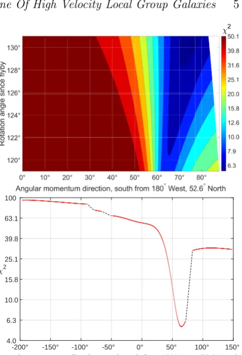
For every value of θ, we vary the rotation angle φ

between 119◦ and 131◦. Each time, we find the value of tanκ_{M W} that minimises the angle between the calculated and observed spin vector of the MW satellite plane. The same procedure is used for M31. We combine these angular differences in quadrature to obtain aχ2 statistic, which we base on an allowance of 10◦ for both satellite planes. Our results are shown in Figure3.

Restricting to anglesφ6131◦, we can obtain a solution withχ2= 5.0 forθ= 75◦,φ= 131◦. Although the resulting

χ2is a little higher than 2, it is still quite acceptable. Our toy model is thus able to provide a plausible explanation for the origins of the MW and M31 satellite planes based on these galaxies having undergone a past close encounter. Naturally, we hope to refine our model in future, perhaps by using the RAyMOND algorithm (Candlish et al. 2015) or the publicly available Phantom of RAMSES algorithm (L¨ughausen et al. 2015), both of which handle MOND explicitly by adapting the RAMSES algorithm (Teyssier 2002). It is already possi-ble to use the latter to simulate interacting disk galaxies in MOND (Thies et al. 2016).

We find that it is much more difficult to explain the orientation of the M31 satellite system than that of the MW. This may be related to the M31 satellite plane being inclined to its disk by ∼47◦ (Ibata et al. 2013) whereas the MW satellite plane is almost polar with respect to its disk (Pawlowski & Kroupa 2013). This makes it more likely that the M31 satellite plane has precessed from its initial orientation (Fernando et al. 2017), especially as the M31 disk has a scale length ∼2.5×larger than that of the MW (Courteau et al. 2011; Bovy & Rix 2013). However, such precession effects would tend to thicken the M31 satellite plane as they would be weaker for satellites further from M31 (Fernando et al. 2017). The very low observed thickness (12.6±0.6 kpc,Ibata et al. 2013) therefore argues against such an explanation.

Due to the different disk-satellite plane misalignments for the MW and M31, our model implies that the MW was more affected by tides from M31 than vice versa (Table2). In MOND, we can obtain a good estimate of the mass of a galaxy from its rotation speedv_f in the flat outer region of its rotation curve (Equation 3). This suggests that the slower-rotating MW withv_f = 180 km/s (Kafle et al. 2012)

-200° -150° -100° -50° 0° 50° 100° 150°

Angular momentum direction, southwards from 180° West, 52.6° North

4.0 6.3 10.0 15.8 25.1 39.8 63.1 100

@2

Figure 3.Top:Goodness of fitχ2 _{of our toy model to the MW} and M31 satellite plane orientations as a function of model pa-rameters, assuming an uncertainty of 10◦_{for both systems. The} best-fitting solution is given in Table2. The gap arises as some models violate Equation 9 and so could not plausibly lead to enough tidal torque on at least one major LG galaxy to explain the misalignment between its disk and dominant satellite plane (Figure15). The issue of most relevance is that the MW seems to have been almost within the M31 disk plane at the time of their closest approach.Bottom:χ2_{as a function of the adopted} MW-M31 orbital plane with a fixed rotation angle ofφ= 131◦since their flyby. The dashed black lines correspond to directions ofbh

for which it is not possible to satisfy the 4 constraints imposed by Equation9, leading to 4 distinct excluded ranges ofθ(one of which has been folded around the figure for clarity).

has a lower mass than the faster-rotating M31 withv_f = 225 km/s (Carignan et al. 2006). As the MW disk is also easier to tilt because it has less specific angular momentum than the M31 disk, it is reasonable to get tanκ_{M W} a few times larger than tanκM31. Therefore, in MOND, the faster

asymptotic rotation speed of M31 is directly related to the larger observed angle between the MW disk and its satellite plane compared to the same quantity for M31 (Figure15).1 This is exacerbated by our model implying that rbM31 at

the time of the flyby lay only ∼6◦ out of the M31 disk plane, reducing how much torque could be exerted on it (Equation8). At that time,rbM31 was ∼66

◦

from the MW

Quantity Value

MW satellite plane spin vector (176.4◦,−15.0◦) M31 satellite plane spin vector (206.2◦,7.8◦) MW-M31 orbital angular 75◦

momentum directionθ

Expected MW-M31 orbital polebh (217.3◦,−15.1◦)

Rotation angle of MW-M31 131◦ line since their flyby,φ

tanκM W (see Figure2) 3.7 tanκM31 (see Figure2) 1.0

Table 2.Values of the quantities most relevant to the geometry of a past MW-M31 flyby and its effects. The MW satellite plane orientation is fromPawlowski & Kroupa(2013, Section 3) while that of M31 is from their Section 4. Other parameters are deter-mined using a toy model of a past MW-M31 interaction forming their planes of satellite galaxies (Section2.2).

disk plane. However, the larger scale length of the M31 disk may have counteracted these factors somewhat. Combining these considerations suggests that

tanκ_{M W}

tanκ_M31 ≈ _v

f,M W

v_f,M31 5_r

d,M W

r_d,M31

sin 66◦cos 66◦ sin 6◦_{cos 6}◦ (11)

≈ 4 (12)

The ratio between the disk scale lengthsr_d of the MW and M31 may have been different in the past and their orien-tations may have been slightly different too. Moreover, our model is only a very basic one. Despite this, Equation 11 suggests that tanκM W ≈4 tanκM31, similar to the ratio in

our best-fitting model (Table2).

For both major LG galaxies, the rather large values of

κsuggest that some material may have been pulled out of them and become unbound. This may explain why some LG non-satellite galaxies have unusual kinematics (Banik & Zhao 2017a). It is possible that the material in some of them was once part of the MW or M31 disk or in their satellite system. Further study of this scenario must be left for future works.

3 THE LOCAL GROUP IN MOND

3.1 Governing equations

We now conduct a more detailed simulation of the LG in MOND, taking advantage of the MW-M31 orbital pole de-termined in Section 2.2. The MW-M31 trajectory is simu-lated by advancing them according to their mutual gravity supplemented by the cosmological acceleration term (e.g. Banik & Zhao 2016, Equation 24).

¨

r_rel = gM31−gM W + ¨

a

arrel where (13)

rrel ≡ rM31−rM W (14) Here, the cosmic scale-factor is a(t) andri is the po-sition vector of galaxy i (MW or M31), at whose location the gravitational field (excluding self-gravity) isg_i. We use an overdot to indicate the time derivative of any quantityq

e.g. ˙q≡∂q_∂t. All position vectors are with respect to the LG barycentre, which we take to be 0.3 of the way from M31 towards the MW. This is based on the asymptotic rotation

curve of the MW flatlining at∼180 km/s (Kafle et al. 2012) while the equivalent value for M31 is ∼225 km/s (Carignan et al. 2006). In the context of MOND, this suggests that the mass of M31 is 225₁₈₀4

≈2.3×that of the MW (Equation 3).

Although MOND is known to work well at explain-ing the internal dynamics of galaxies outside the LG (e.g. Famaey & McGaugh 2012), we should check if this is the case for the MW and M31 before using it to determine the gravity they exert on each other and on the rest of the LG. For our neighbour M31, MOND can provide a fairly good match to its rotation curve using its observed baryonic distribution (Corbelli & Salucci 2007, Figure 4). For our work, it is im-portant to note that this fit remains good out to rather large radii (∼35 kpc or 7 disk scale lengths). A similar analysis for the MW is complicated slightly by our position within its disk. However, it has recently become clear that MOND can explain its rotation curve fairly well (McGaugh 2016a) and even provides a good match to its escape velocity curve (Banik & Zhao 2017b). Thus, applying Equation 3 to the MW and M31 rotation curves yields reasonable estimates for their baryonic masses, the vast majority of which resides in stars (91% for M31 and 81% for the MW,Yin et al. 2009, Section 2.2). This is almost certainly not representative of the Universe as a whole given that most of the mass in galaxy clusters is hot gas that has only recently been discovered at X-ray wavelengths (e.g. Vikhlinin et al. 2006). Indeed, the location of all the baryons in the Universe is far from certain, with significant amounts perhaps residing in an even more diffuse form (Nicastro et al. 2008).

Having obtained MW and M31 masses (MM W and

MM31) in this way, we treat them as point masses and find

the gravitational fieldgthey exert at position r using the quasilinear formulation of MOND (Milgrom 2010). We as-sume the ‘simple’ interpolating function between the New-tonian and deep-MOND regimes (Famaey & Binney 2005) that works best for the MW rotation curve (Iocco et al. 2015).

gN ≡ −

X

i=M W,M31

GMi(r−ri)

|r−r_i|3 (15)

∇ ·g ≡ ∇ ·

ν

|g_N|

a₀

g_N

where (16)

ν(x) = 1 2 +

r

1 4+

1

x (17)

The appropriate boundary conditions are similar to Newtonian gravity, but for definiteness we give them here.

∇ ×g = 0 (18)

g → 0 as |r| → ∞ (19)

We use direct summation to obtaing from its diver-gence.

g(r) =

Z

∇ ·g r0 (r−r 0

) |r−r0_|3 d

3

r0 (20)

At larger distances, we assume that the MW and M31 can be treated as a single point mass located at their barycentre, yieldingg=νg_N.

3.2 MW-M31 trajectory

Using the gravitational field thus found, we integrate the MW-M31 trajectory backwards from present conditions. In general, the galaxies will not be on the Hubble flow at the start time of our simulationsti, when the cosmic scale-factor

ai = 0.05 and the Hubble parameterH≡ ˙

a

a isHi. However, deviations from the Hubble flow are observed to be very small at early times (Planck Collaboration 2014). In order to satisfy this condition atti, we vary the total mass of the MW and M31 using a Newton-Raphson root-finding algorithm. This ensures that

˙

r_rel =H_ir_rel whent=t_i (21) The MW and M31 are not on a purely radial orbit. Their mutual orbital angular momentum prevents them from con-verging onto the Hubble flow at very early times. This is unrealistic as any non-radial motion must have arisen due to tidal1 _{torques well after the Big Bang. Thus, we take}

the MW-M31 orbit to be purely radial prior to their first turnaround att≈3 Gyr. After this time, we assume their trajectory conserves angular momentum at its present value. This implies the MW-M31 angular momentum was gained near the time of their first turnaround, when their large separation would have strengthened tidal torques. At later times, the larger scale factor would weaken tidal torques, suggesting that these have a much smaller effect around the time of the second MW-M31 turnaround than the first.

At present, there is no detailed theory for structure for-mation in MOND because it is unclear how to apply it to regions only slightly denser than the cosmic mean density. Assuming a particular model, structure formation was found to be more efficient than in ΛCDM (Llinares et al. 2008). Observationally, there are several indications that this is ac-tually the case (Peebles & Nusser 2010), including the rather high fraction of pure (bulgeless) disk galaxies (Kormendy et al. 2010).

Thus, structure formation in MOND − and perhaps in the Universe−is not so reliant on growth at late times through mergers, which would be less efficient in MOND due to the absence of dynamical friction between extended dark matter halos. Instead, galaxies would form relatively rapidly after the Big Bang, emptying their surroundings due to the strong long-range gravitational attraction in the model. This would lead to many widely separated ‘island universes’ with fairly empty intervening voids, perhaps similar to the Local Volume (out to 8 Mpc) which does seem to contain voids emptier than might be expected in ΛCDM (Tikhonov & Klypin 2009). With mass draining on to a few well-separated massive galaxies, it would be natural for the MW and M31 to end up fairly isolated. Thus, there would not be much tidal torque on the MW-M31 system, leaving its orbit close to radial. This suggests that it would not be all that unusual for us to find ourselves in a galaxy which had a past close

1 _{affecting the MW and M31 differently}

0 2 4 6 8 10 12 14

Time since Big Bang, Gyr

0 0.2 0.4 0.6 0.8 1

MW-M31 separation, Mpc

Figure 4.MW-M31 separation in our MOND simulation, show-ing a past close flyby 6.59 Gyr after the Big Bang at a closest approach distance of 14.17 kpc. At that time, their relative veloc-ity was 716 km/s, of which 501 km/s was due to motion of the MW. The higher second apogalacticon is partly due to the effect of cosmology (Equation13) and our assumption that the MW and M31 lose 5% of their mass around the time of their encounter (see text).

encounter with its nearest large neighbour if structure for-mation proceeded more efficiently than in ΛCDM. Of course, it remains to be seen whether it forms too efficiently in MOND.

Given the way we expect structure to form in MOND, we assume the MW and M31 masses do not grow by accre-tion at late times. However, an important effect included in our models is a 5% reduction in their masses at the time of closest approach, when their simulated separation was just 14.2 kpc.2 _{Considering that the MW disk has a scale}

length of 2.15 kpc (Bovy & Rix 2013) while the correspond-ing quantity for M31 is 5.3 kpc (Courteau et al. 2011), it is very likely that some of the mass in these galaxies would be expelled to large distances and escape from them.

This mass could reside in the halos of hot gas sur-rounding each galaxy. Such a halo has been detected around M31 based on absorption features in spectra of background quasars (Lehner et al. 2015). A similar halo is thought to be necessary around the MW to explain the truncation of the Large Magellanic Cloud’s gas disk (Salem et al. 2015). These gas halos seem to contain perhaps 3×1010_M

each, with much larger amounts being very unlikely given constraints from the MW escape velocity curve (Banik & Zhao 2017b). Considering that the MW rotation curve flatlines at ∼180 km/s (Kafle et al. 2012) while that of M31 flattens at ∼225 km/s (Carignan et al. 2006), MOND suggests their total baryonic mass is 2.3×1011M. This makes it quite feasible for them to have lost 1010_M

of hot gas around the time of their encounter, as our model implies. Some hot gas in an extended halo could also explain why the rotation curve-based estimate of the total MW and M31 mass falls a little

below our timing argument estimate of 2.9×1011_M (for simplicity, we fix the MW:M31 mass ratio at 3:7 and scale up their masses slightly to make the timing argument work). There are several other aspects of the problem which we include in our model using techniques we developed. We defer a more detailed explanation of our procedures to a forthcoming publication which will investigate the MW-M31 trajectory in MOND. For the present contribution, the major result is that Equation 21 can be satisfied by backwards integration from present conditions using MW and M31 masses consistent with their rotation curves in MOND (themselves consistent with observed baryonic disk masses) and the more extended halos of hot gas that have recently been detected around them (Lehner et al. 2015; Nicastro et al. 2016). The resulting MW-M31 trajectory is shown in Figure 4. A past close encounter is inevitable in the context of MOND (Zhao et al. 2013) due to their slow relative tangential motion (van der Marel et al. 2012a) and the strong gravity in this model. We previously discussed how the thick disk of the MW and the LG satellite planes may well have formed due to this interaction (Sections1and 2.2, respectively). Here, we consider its effect on the rest of the LG.

3.3 Test particle trajectories

Once the MW-M31 trajectory is known, we can determine the gravitational field g everywhere within the LG at all times under the assumption that only these point masses are present in an otherwise homogeneous Universe. This allows us to advance the trajectories of test particles according to

¨

r = ¨a

ar + g (22)

˙

r = H_ir whent=t_i (23) Although the particles could not have started exactly on the Hubble flow, we consider this a reasonable assumption for reasons we now discuss. The MW and M31 could not have formed much earlier than whena= 0.05 because the MOND free-fall collapse time on to a point mass is given by

tf f =

r0

vf

r π

2 (24)

v_f is given by Equation3and taken to be 180 km/s for the MW (Kafle et al. 2012). Assuming the material currently in it must have turned around from a distance & 100 kpc (Equation 27), this yields a free-fall timescale of tf f = 540 Myr. This is much more than the 191 Myr age of the Uni-verse whena= 0.05 in standard cosmology, suggesting that it is not appropriate to start our simulations much earlier.

Moreover, even if the MW existed as a point mass since the Big Bang, the resulting peculiar velocity some co-moving distancedaway would be

avpec ≡ a vpec

z }| {

( ˙r−Hr) =

Z t

0

ag dt where (25)

g =

p GM a0

ad (26)

The integrating factor a(t) accounts for the effects of Hubble drag. We have assumed that the particle nearly fol-lows the Hubble flow so that its distance to the mass can

be taken as a(t)d. At a co-moving distance of 2 Mpc, the peculiar velocity gained would only be 65 km/s by the time

a= 0.05. At that time, the Hubble velocity of the particle was nearly 340 km/s, justifying our assumption that it was almost on the Hubble flow.

To understand the effect on the present-day velocity field, we must bear in mind that both the present position and velocity of a test particle would be affected if we get its velocity wrong at some earlier time. Thus, if we wish to know the velocity at a particular position today, we would need to consider a different test particle starting at a different posi-tion. This ‘initial condition drag’ scales down the effect of a velocity error at earlier times (when the scale factor wasa) on the present velocityat fixed positionby a factor of∼a2.4

(Banik & Zhao 2016, Figure 4). However, even if we make the more conservative assumption that it simply scales with

a (like traditional Hubble drag), a 65 km/s velocity error when a = 0.05 would only affect the present LG velocity field by ∼3 km/s. This is probably why our axisymmetric dynamical model of the LG was hardly affected by using a different start time (Banik & Zhao 2016, Section 4.6). Thus, our choice of initial conditions should be sufficient to get an approximate idea of how the LG might have been affected by a past MW-M31 flyby. Moreover, the fact that motions at high redshift have only a weak impact on our results implies that they should be robust to uncertainties surrounding the application of MOND in a cosmological context (at lower redshifts, the MW and M31 have already formed and so better approximate the isolated situations where it is clear how MOND works).

Because the MW and M31 must have accreted matter from some region prior to the start of our simulation, we exclude all test particles starting within a distancer_exc,i of galaxyi. We determine this by requiring that the excluded volume has as much baryonic matter as galaxy i, taking the density of baryons to be the cosmic mean value. This is obtained from the fraction Ωb,0 = 0.049 that baryons

currently comprise of the cosmic critical density, which we found by taking H0 ≡ H(t0) = 67.3 km/s/Mpc (Planck Collaboration 2016, Table 4). The cosmic baryon density can be estimated using Big Bang nucleosynthesis arguments− only a narrow range of values is consistent with the primor-dial abundances of light elements such as deuterium (Cyburt et al. 2016).

4π

3 rexc,i

3

×

Baryon density att_i

z }| {

3H0 2

8πGΩb,0ai −3

≡ Mi (forrexc,i) (27)

For consistency, it is necessary that the sizes of the ex-cluded regions satisfy

r_{exc,M W} + rexc,M31 6 |rrel| whent=ti (28) This inequality applies becauserexc is 77.7 kpc for the MW and 102.5 kpc for M31, leading to a total of 180.2 kpc − interestingly, this is just smaller than r_rel(t_i) = 182.1 kpc, suggesting that the two galaxies accreted matter from regions which just touched. This remains the case if we use a slightly different start time as rexc,i ∝ a_i, similarly to

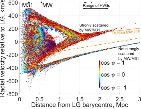
Figure 5.Hubble diagram of the test particles in our simulation coloured by their value of cosψ, which parametrises how well their orbital angular momenta align with that of the MW-M31 orbit (Equation30). We show the Hubble flow line (solid orange) and a 1.5×steeper line (dashed orange) which we use to select analogues of HVGs in later figures. Particles below this line have generally never interacted closely with the MW or M31, unlike particles above the line. The black dots along the top edge of the figure indicate distances to the MW, M31 and the HVGs. Marker sizes have been enlarged in some regions for clarity, but do not correspond to volume factors (see text). Thus, particles at distances.1 Mpc represent much less mass than it might appear.

3.4 Simulation results

In Figure 5, we show the distances and radial velocities of test particles with respect to the LG barycentre, colour-coding them according to the orientation of their orbital plane. We quantify this based on the specific angular mo-mentumh, whose direction can readily be compared with the MW-M31 orbital polehb_{M W−M31}.

h ≡ r×r˙ (29) cosψ ≡ bh·hb_{M W−M31} (30)

The initial positions of the particles span a grid in spher-ical polar co-ordinates. We do not show results for particles that pass within 15.4 kpc of the MW or 21.5 kpc of M31. In the real LG, such particles would likely have merged with the nearby galaxy.

For this work, the important feature is the upper branch of the Hubble diagram. Its upward slope arises because these particles must have passed close to the spacetime location of the MW-M31 encounter and gained a substantial amount of kinetic energy in what was essentially a 3-body interaction. Thus, for such particles to be further away from the LG now, they must have a larger outwards velocity. This will depend somewhat on when each particle approached whichever of the MW or M31 most strongly scattered that particle − and thus the speed of the perturber at that time.

However, the precise encounter distance b should not affect our results much because of ther−1gravity law (Equa-tion 1). Roughly speaking, doubling b halves the strength of gravity but doubles the duration of the encounter, leav-ing the total impulse unchanged. This is probably why we

0 5 10 15 20 25 30 35 40 45 50

Closest approach distance to MW or M31, in disk scale lengths

0 0.02 0.04 0.06 0.08 0.1 0.12 0.14

Fraction of high-velocity particles >1.6 Mpc away

Figure 6.Histogram of the closest approach distances of high-velocity test particles (above dashed orange line in Figure5) to the MW or M31 in units of their disk scale lengths. We show whichever of these quantities is smaller for any given test particle. It is evident that very few of these particles approached the MW or M31 so closely for the details of their mass distribution to become important. Each particle has been weighted according to the volume it represents in our 3D grid of initial conditions. This corresponds to the mass it represents if we assume that the LG initially had a uniform density except in appropriately sized spherical ‘holes’ around the MW and M31 (Equation27).

found no clear correlation between how far particles were flung from the LG and how closely they approached the MW/M31. Thus, our results should not depend much on the minimum allowed encounter distance in our simulation or on the fact that the MW and M31 have finite extents and are not point masses. The important effect here is the time dependence of the gravitational field at the positions of the test particles which get flung out at high speed. Most of these never come that close to the MW or M31 because the commoner more distant encounters are just as effective at scattering test particles (Figure6).

ΛCDM also allows slingshot encounters with the MW and M31, but their fairly slow motion means that they can only fling galaxies out to ∼1 Mpc from the LG, at which point the upper branch of the Hubble diagram simply stops (Banik & Zhao 2016, Figure 3). Even in more detailed cosmological simulations of ΛCDM that include encounters with satellites of MW and M31 analogues, dwarf galaxies do not get flung out beyond this distance (Sales et al. 2007, Figures 3 and 6). For MOND, the corresponding limit is ∼2.5 Mpc due to the MW-M31 flyby, which therefore makes a dramatic difference to the Hubble diagram at distances of ∼1−2 Mpc (Figure5). In this distance range, our simula-tion yields a bimodal distribusimula-tion of radial velocities, with the HVGs corresponding to particles in the upper branch.

Figure 7.Histogram of cosψfor all high-velocity test particles (above dashed orange line in Figure5) beyond 1.6 Mpc from the LG barycentre in order to best correspond to actual HVGs (Figure 10). The dashed blue line indicates that 0.025 of the (weighted) particles should fall into each bin in cosψ if their orbital poles were distributed isotropically.

1 1.5 2 2.5 3

Distance from Local Group barycentre, Mpc

0 0.2 0.4 0.6 0.8 1

Fraction of high velocity particles with |cos

A

| > 0.9

Figure 8.Fraction of high-velocity test particles (above dashed orange line in Figure 5) in each radial bin which have|cosψ|> 0.9. The dashed white line shows the expectation for an isotropic distribution (0.1). Notice how the high-velocity particles furthest from the LG now tend to have a more anisotropic distribution. Uncertainties are estimated using binomial statistics, though this is not totally accurate due to our statistical weighting scheme (see text). The result for the outermost radial bin is less reliable as we only have 24 particles in it, but other bins have at least 96 and should be quite reliable.

field of large scale structures on the LG. This external field effect weakens the gravity exerted by the MW and M31 at long range (e.g. Banik & Zhao 2015). It is not caused by tides but arises because MOND gravity is non-linear in the matter distribution (Equation17).

In most parts of our simulated Hubble diagram, a mod-erate fraction of particles have orbits poorly aligned with the MW-M31 orbit (points coloured light blue, green or yellow in Figure5). However, this is not true for the high-velocity branch at distances& 1.5 Mpc, which appears almost

en-0 0.5 1 1.5 2 2.5 3

Distance from MW-M31 orbital plane, Mpc

0 0.02 0.04 0.06 0.08 0.1 0.12

Fraction of high-velocity particles

Low velocity particles High velocity particles

Figure 9. Histogram showing how far simulated particles are from the MW-M31 orbital plane. We only show particles currently at distances of 1.6−3 Mpc from the LG and sort them according to whether they are in the high-velocity branch of the Hubble diagram (above dashed orange line in Figure5). If they are, we show them as red. The remaining particles (shown in blue) are well described by an isotropic distribution (dashed grey line).

tirely dark red (cosψ ≈ 1). This leads us to do a care-ful analysis of whether such particles really are distributed anisotropically.

Our initial grid of test particle positions is uniform in distance from the LG as well as in the spherical polar and azimuthal angles. Thus, each particle does not correspond to exactly the same volume/mass. We handle this by weighting each particle according to the volume it represents, which we find by integrating the usual spherical Jacobian factor over the range of initial co-ordinates covered by the particle1.

We apply this weighting scheme to the high-velocity particles (above dashed orange line in Figure5) to determine their correctly weighted distribution over cosψ (Figure 7). If the particles have no preferred direction(s), then cosψ

should be distributed uniformly. Because we are investigat-ing HVGs towards the edge of the LG, we also restrict to particles beyond 1.6 Mpc from its barycentre (as suggested by Figure10).

A large proportion of high-velocity particles appear to have very high values of|cosψ|. To see how robust this is, we determine the (weighted) fraction of particles in different radial bins with|cosψ|>0.9, our proxy for an orbital plane almost aligned with that of the MW and M31. We esti-mate uncertainties using binomial statistics, which is only approximately correct here due to our weighting procedure. Apart from the outermost radial bin, there should be enough simulated particles in each one to accurately estimate this fraction.

Compared to an isotropic distribution, the fraction of nearly co-planar particles is very high (Figure 8). This demonstrates that dwarfs flung out furthest from the LG should be distributed very anisotropically in a MOND

text. Moreover, the preferred plane should correspond to the MW-M31 orbital plane. Within this plane, the HVGs should mostly be co-rotating with respect to the MW-M31 orbit (Figure7). However, it is not possible to test counter-rotation vs co-counter-rotation at present due to a lack of accurate proper motions for the HVGs. This is why we focus on|cosψ| rather than cosψ.

Gravitational slingshot interactions with the MW or M31 would be most efficient for particles flung out almost parallel to the motion of the perturber. Considering that the MW-M31 flyby occurred a fixed time in the past, these particles should currently be furthest away from the LG. Thus, it is not very surprising that the spatial distribution of such particles is highly flattened with respect to the MW-M31 orbital plane (Figure9).

Although this scenario almost exclusively leads to HVGs co-rotating with respect to the MW-M31 orbit, that is not always the case. For a particle flung out on an almost radial orbit with respect to the LG, only a small torque is needed to reverse the direction of its angular momentum. This may explain why the high-velocity test particles with cosψ ≈ −1 tend to have rather small angular momenta. Pawlowski et al. (2011) suggested a similar mechanism to explain why some MW satellites like Sculptor are counter-rotating within the plane preferred by most remaining MW satellites (Piatek et al. 2006).

4 THE LOCAL GROUP INΛCDM

4.1 Refining theΛCDM model

To better identify which galaxies may have been flung out by a fast-moving MW/M31 in the way discussed in Section 3, we refine our previous ΛCDM dynamical model of the LG (Banik & Zhao 2017a). In this work, we use an updated input catalogue. The main changes are a more accurate distance measurement to NGC 404 (Dalcanton et al. 2009) and to Leo P (McQuinn et al. 2015). For NGC 4163, we use a less accurate distance of 2.95±0.07 Mpc to bracket the range between the measurements of Dalcanton et al. (2009) and Jacobs et al.(2009), both of which are based on data from the Hubble Space Telescope.

We also make improvements to the procedure used to find the best-fitting model parameters. The flatline level of the MW rotation curve is no longer assumed equal to its amplitudevc,at the position of the Sun.1 We let the for-mer vary with a prior of 205±10 km/s (McGaugh 2016a) whilevc,is fixed at 232.8 km/s (McMillan 2017). The time resolution is improved 10×so that 5000 steps are now used to cover the history of the Universe since redshift 9 (a= 0.1), leading to a much better handling of close encounters.

The best-fitting solution is found by applying gradient descent to all model parameters, using a method similar to that described in Section 5.1. To maximise the chance of matching observations, we run a grid search through the tra-jectories of all the dwarf galaxies, which are treated as test particles. Because the algorithm uses a least action method (Peebles et al. 2011), trajectories are solved by relaxing an initial guess towards a solution that satisfies the equations of

1 _{This is sometimes called the Local Standard of Rest (LSR).}

0 0.5 1 1.5 2 2.5 3 3.5

Distance from LG barycentre, Mpc

-100 -50 0 50 100 150

GRV adjusted for GA, km/s

Sextans B Sextans A

Leo P

Tucana

Sagittarius HIZSS 3

NGC 55 KKH 98

KKH 86 DDO 190

NGC 4163 Cetus

Andromeda Leo A WLM

Antlia NGC 3109

KKR 25 _{IC 5152} ESO 294-G010

GR 8 DDO 125 KKR 3 IC 3104

UGC 9128

IC 4662 UGC 8508

DDO 99 DDO 216

Aquarius

UGC 4879

NGC 300

UKS 2323-326

NGC 404

Figure 10.The deviation ∆GRV of each target galaxy from our best-fitting ΛCDM model is shown against its distance from the LG barycentre. If the model worked perfectly, then all galaxies would have ∆GRV ≡0 (dot-dashed line) as model predictions are subtracted. Given likely model uncertainties of ∼25 km/s (Aragon-Calvo et al. 2011), ΛCDM would thus find it difficult to explain galaxies with ∆GRV >50 km/s (above solid black grid-line). In our MOND scenario of a past MW-M31 flyby, we expect the HVGs to broadly follow a trend of 50 km/s/Mpc (diagonal grey line) and to reach distances up to ∼2 Mpc (Figure5).

motion. The initial guess has the co-moving position varying linearly witha. The direction and magnitude of the present peculiar velocity of each dwarf are varied over a 3D grid of possibilities, giving the algorithm a much better chance of finding slingshot encounters that might otherwise get missed if the initial trajectory went nowhere near the spacetime location of the encounter. The issue of local but not global minima can always be solved with a grid search, which in this case is feasible for the dwarf galaxies because the trajectory of each one does not influence the gravitational field in the LG and thus the trajectory of anything else.2

As some improvements are indeed found in this way, we repeat the gradient descent stage and the grid search in an alternating manner until the algorithm converges in the sense that the grid search stops improving the agreement between model and observations. This process takes a few days and yields reliable trajectories for all simulated galax-ies −their present-day positions and velocities are almost perfectly recovered (maximum errors of 9 pc and 16 m/s, respectively) if we solve their trajectories forwards using a more traditional fourth-order Runge-Kutta method with 10×finer resolution.

Using Equation 30 fromBanik & Zhao(2017a), we ad-just the predictions of this best-fitting model for the effect of tides raised on the LG by the Great Attractor. This only slightly affects our results, which are shown in Figure10. The main difference from our previously published results (Banik & Zhao 2017a, Figure 13) is that Tucana is now consistent with ΛCDM expectations.

At distances &1.5 Mpc, a bimodal distribution of ∆GRVs is apparent, similar to that in our MOND simu-lation of the LG (Figure 5). Moreover, the galaxies in the lower branch predominantly have ∆GRV < 0, perhaps a sign of the stronger gravity in MOND than in the ΛCDM model whose predictions have been subtracted.

4.2 Selecting high-velocity galaxies

To find HVGs in the real LG, we compare the distances d

of our target galaxies from the LG barycentre with their ∆GRV ≡ GRVobs−GRVmodel relative to our best-fitting 3D dynamical model of the LG (Figure10). We expect that these dwarf galaxies were flung out at high speed by the MW or M31, implying they passed close to the spacetime location of the MW-M31 flyby. Thus, such dwarfs should follow a ∆GRV ∝_∼ d relation of the sort apparent in our MOND simulation of the LG (Figure5). A relation like this is evident in Figure10, where we have added a solid grey line at u= 50 km/s/Mpc to make it clearer. A radial velocity excess of this magnitude suggests that the MW-M31 flyby occurred∼(H0+u)

−1

≈8 Gyr ago. This is consistent with their expected orbital evolution in MOND (Figure4).

A larger MW-M31 pericentre would not affect this con-clusion much as a HVG would still require a similar velocity to reach its presently observed position from the spacetime location of the MW-M31 flyby, the timing of which is con-strained observationally if we assume this event led to the formation of the MW thick disk (Quillen & Garnett 2001). However, a weaker MW-M31 encounter would reduce the maximum distance at which we might expect to see a HVG. As our ΛCDM-based model of the LG is not a per-fect representation of a ΛCDM universe, we expect model uncertainties of ∼25 km/s based on how a LG analogue deviates from spherical symmetry in a detailed cosmological simulation of ΛCDM (Aragon-Calvo et al. 2011).1 Thus, we focus our attention on the galaxies with ∆GRV >50 km/s and following the ∆GRV ∝_∼ d relation. This leads to the HVG sample in Table3.

The reasonably high ∆GRV of DDO 190 (66±7 km/s) is still marginally compatible with our model if we assume a model uncertainty of ∼25 km/s. This is especially true when considering that the much larger distance of DDO 190 from the LG barycentre suggests that it should have a much higher ∆GRV if it really was flung out in the same way as e.g. NGC 3109. Thus, we do not consider DDO 190 as being a genuine HVG, even though its ∆GRV is slightly on the high side.

Although it would be quite normal to have one such instance amongst our 34 LG target galaxies of observations exceeding model predictions by 2.6σ(probability≈0.13), a second such instance would be unexpected. Thus, it would be rare to observe ∆GRVs as large as for DDO 190 and KKH 98 (66±9 km/s) if we treat both as having normal kine-matics in a ΛCDM context. Given that DDO 190 deviates very substantially from the ∆GRV ∝ d relation typically followed by HVGs, this suggests that KKH 98 may be a HVG. Although it does not fit the ∆GRV ∝ d relation

1 _{This is discussed in more detail in Section 4 ofBanik & Zhao} (2016).

Galaxies included Distance from MW-M31 ∆GRV, km/s in our plane fit mid-point, Mpc

Milky Way 0.382±0.04 NA

Andromeda 0.382±0.04 3.5±9.1 Sextans A 1.624±0.036 96.1±6.3 Sextans B 1.661±0.037 79.9±6.0 NGC 3109 1.631±0.014 105.0±5.3

Antlia 1.642±0.030 59.7±6.1

Leo P 1.80±0.15 79±14

KKH 98 2.160±0.033 65.5±9.1 Table 3.Galaxies considered when finding the plane best fitting the high ∆GRV galaxies in our sample, which we select based on Figure10.

perfectly, some scatter about this is expected because the LG is not spherically symmetric and is presently observed from an off-centre vantage point. Because most HVGs lie at rather similar angles to the MW-M31 line, we expect larger deviations from this relation for HVGs like KKH 98 which lie at a totally different angle (Figure16).

For the particular case of KKH 98, its position rather close to the MW-M31 line means that its ∆GRV would be more sensitive to where our model puts the centre of mass of the LG i.e. its preferred MW:M31 mass ratio. If the MW and M31 masses are not equal but only 0.3 of their total mass is in the MW (Section3), then the LG barycentre would be shifted by ∼160 kpc towards M31 and thus by a similar amount towards KKH 98. This would put it closer to the LG barycentre. In the LG, the radial velocity rises with distance at a rate close to 100 km/s/Mpc due to the gravity of the MW and M31 (Banik & Zhao 2017a, Figure 5). Thus, a galaxy 160 kpc closer to the LG barycentre should be reced-ing away from it 16 km/s slower. Moreover, the MW would be moving 22 km/s faster towards M31 (and thus KKH 98) given the observed MW-M31 relative radial velocity (van der Marel et al. 2012a). A more massive M31 would also be expected to reduce GRVs of objects in the general vicinity of KKH 98 compared to a situation where the MW and M31 have equal mass. Even without this dynamical effect, the kinematic effects alone would reduce the predicted GRV of KKH 98 by ∼40 km/s but would have a smaller effect on the other HVGs and DDO 190 as their sky positions are almost orthogonal to the MW-M31 line (Figure16). If this is correct, it explains why the ∆GRV of KKH 98 falls below the ∆GRV ∝drelation by about this much.

5 ANALYSING THE LOCAL GROUP

5.1 Finding the best-fitting plane

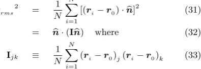
To quantify whether a set of galaxies is distributed anisotropically, we need to define a measure of anisotropy and determine how unusual its value is. The statistic we will use iszrms, the root mean square (rms) of the minimum dis-tances between the galaxies we consider and the best-fitting plane through them (i.e. the one that minimisesz_rms). With respect to a plane having normalnband containing the vector

r₀, the vertical dispersion is

zrms 2

= 1

N N X

i=1

[(ri−r0)·nb] 2

(31)

= n_b·(In_b) where (32)

Ijk ≡

1

N N X

i=1

(ri−r0)j(ri−r0)k (33)

The galaxies are at heliocentric positionsri. The mini-mum ofz_rms is attained whenr₀= 1

N PN

i=1ri, correspond-ing to the geometric centre of the N galaxies to which we are trying to fit a plane. We find the best-fitting orientation

b

nusing a gradient descent method (e.g. Fletcher & Powell 1963). The gradient of zrms

2 _{with respect to} b

n is 2

N(Inb)

less the component of this parallel tonb. At the minimum of zrms, its gradient vanishes, implying thatnbis an eigenvector

of the inertia tensorIcorresponding to its minimum eigen-value. This provides a non-iterative way of minimisingzrms, taking advantage of the characteristic polynomial ofIbeing a cubic whose roots can be found analytically. However, we find that this approach is slower than gradient descent, a much more general method which we also used in Section 4.1.

We minimise issues of local minima by starting the gra-dient descent based on whichevern_byields the smallestzrms in a low resolution grid of possible directions for n_b. Once the angular step size is below 0.006◦, we stop doing further iterations. As well as ensuring that our algorithm always converges in this sense, we also verify it using mock data designed to lie close to a plane with knownn_bandzrms. We are always able to accurately recover their input values.

5.2 Statistical analysis

The MW, M31 and all but one of the HVGs lie close to a plane (Figure 11). We need to reflect this when determin-ing the likelihood ofzrms being as low as the observed 101 kpc. To see if this is consistent with isotropy, we conduct a series of Monte Carlo (MC) trials in which we randomise the directions to these galaxies and recomputezrms. Thus, the probability distribution of the Galactic longitude l is uniform while that of the Galactic latitudebis

P(b)db = 1

2cosb db (34)

To mimic uncertainties in measured distances to LG galaxies, we randomly vary their heliocentric distances using Gaussian distributions of the corresponding widths. In the very rare cases where this yields a negative distance, we set this to 0.

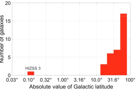
To account for HIZSS 3 being excluded from our plane fit despite its high ∆GRV, we use the procedure described

Quantity Full sample Without Antlia

Galaxies in plane 8 7

Normal to plane of

204.4◦ −30.1◦

206.6◦ −31.8◦

high ∆GRV galaxies

rms plane width, kpc 101.1 101.9 Aspect ratio (Eq.35) 0.0763 0.0750 MW offset from plane 224.7 195.4 M31 offset from plane -0.6 -12.8 Angle of MW-M31

16.2◦ _14.9◦ line with plane

Table 4.Information about the plane best fitting the galaxies listed in Table3, with distances in kpc and plane normal direction in Galactic co-ordinates (latitude last). The last column shows how our results change if Antlia is removed from our sample as it could be a satellite of NGC 3109 (van den Bergh 1999). The effect on our statistical analysis is described in Section6.4.

in Section 5.1to find the best-fitting plane through every combination of all HVGs but one as well as the MW and M31.1 _{The combination yielding the lowest z}

rms is consid-ered the analogue of the observed HVG system less HIZSS 3 for that particular randomly generated mock catalogue. In Section6.5, we perform calculations where we select the combination yielding the lowest aspect ratioA rather than

zrms.

A ≡ zrms

p

rrms2−zrms2

where (35)

rrms 2

≡ 1

N N X

i=1

|ri−r0| 2

= T race(I) (36)

rrms is the rms distance of the galaxies from their geo-metric centrer₀. To get the rms extent of the system after projection into the best-fitting plane, we need to subtract

zrms in quadrature. Dividingzrms by the result then gives a measure of the typical ‘vertical’ extent of galaxies out of this plane relative to their ‘horizontal’ extent within it. We would obtain identical probabilities for the observed situation if we definedAaszrms

r_rms instead, as long as it is defined in the same

way for the actual HVGs and the mock sample in each MC trial (Section5). This is becauseAis a monotonic function of zrms

r_rms with either definition.

The major LG galaxies along with the HVGs except HIZSS 3 (full list in Table3) define a rather thin plane whose parameters are given in Table4. This allows us to compare the ∆GRV of each galaxy2with its minimum distance from this plane. The galaxies in our full sample have a wide range of positions relative to it, with a similar number on either side (Figure11). However, the HVGs tend to lie very close to it. The only exception is HIZSS 3, justifying our decision not to consider it when defining the HVG plane. In any case, the observations for HIZSS 3 are rather insecure (Section6.3).

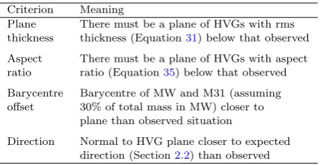
In Table 5, we give the criteria which we use to de-termine whether the distribution of HVGs in a MC trial is analogous to their observed distribution. We choose these criteria so that they should be satisfied if the LG behaves