Distributed Processing for Operational Modal Analysis of Bridge Infrastructures Using Wireless Sensor Networks

(1)

(2)

Master Thesis

Distributed Processing for

Operational Modal Analysis of

Bridge Infrastructures Using

Wireless Sensor Networks

Alkindi Rizky Dzulqarnain

s1595105

supervised by :

Prof. Dr. P.J.M. Havinga

Dr. Ir. Nirvana Meratnia

Dr. Ir. Richard Loendersloot

(3)

Acknowledgements

I would like to express my gratitude to Paul Havinga and Nirvana Meratnia for the patience, guidance, and feedbacks throughout the duration of my the-sis work. I would also like to thank Richard Leondersloot for all of the helps whenever I have problems in understanding or interpreting things related to applied mechanics and modal analysis.

Furthermore, my thanks to LPDP Scholarship from Ministry of Finance of Indonesia for giving me the opportunity to study in University of Twente. Also, thanks to my family and friends for their continuous support through-out my study in the Netherlands.

(4)

Abstract

The modal parameters of a structure is useful for various reasons, such as finite element model checking or structural damage detection. For large structure such as bridge, where controlled vibration excitation is not pos-sible and only operational vibration data can be used, so-called operational modal analysis (OMA) are used to estimate the modal parameters from struc-tural vibration. In the recent years, there is a trend of using wireless sensor network for continuous OMA of structural health monitoring due to its ease in installation and maintenance. However, understanding the large amount of data produced from structural vibration and energy constrain of wire-less sensor node, simply sending raw vibration data to central node means less lifetime for sensor node. Therefore, it is preferable to perform as much as possible OMA processes locally on sensor node such that sensor node only transmit meaningful or transformed data. Based on this, an automatic distributed OMA based on Frequency Domain Decomposition (FDD) is pro-posed. Unlike centralized FDD, the FDD is only applied to a set of small areas surrounding natural frequencies instead of full frequency range. By per-forming FFT operation locally on sensor node, each sensor node only send reduced FFT result data, correlated to the selected area, to the central node. Experiment on three real bridge shows that the method could reliably detect correct modal parameters and reduce the transmitted data size into 1.27 per-cent of its time-domain vibration signal data size. The practical feasibility review also shows that its implementation on wireless sensor node consumes minimum amount of RAM, processing power, and energy consumption. The result shows that lifetime of sensor node is estimated to be able to exceed one year using only 2000 mAh battery.

Keywords : operational modal analysis, frequency domain decomposition, distributed process, wireless sensor network

(5)

List of Figures

2.1 Overview of FDD Process . . . 7

2.2 Example of Singular Value Plot . . . 8

2.3 Example PSD plot from three sensors . . . 9

2.4 First Phase Process of Distributed FDD . . . 10

2.5 First Phase Peak Selection Process . . . 11

2.6 First Phase Peak Area Construction Example . . . 12

2.7 Second Phase Process of Distributed FDD . . . 13

2.8 Second Phase Result Example . . . 14

2.9 Third Phase Peak Selection Process . . . 16

3.1 Photos of Pit Bridge Structure . . . 18

3.2 Sensor placement on Pit Bridge Structure . . . 18

3.3 Vibration Signal Example of Pit Bridge Measurement . . . 19

3.4 Second Phase Result Plot of Pit Bridge Experiment . . . 19

3.5 Mode Shapes of Pit Bridge Experiment . . . 20

3.6 Photos of Steel Arch Bridge Structure . . . 22

3.7 Sensor Placement Photos on Arch Bridge Structure . . . 23

3.8 Sensor Placement Diagram on Arch Bridge Structure . . . 23

3.9 Vibration Signal Example of Steel Arch Bridge Measurement . 24 3.10 Second Phase Result Plot of Steel Arch Bridge Experiment . . 24

3.11 Mode Shapes of Steel Arch Bridge Experiment . . . 26

3.12 Railing Connection on Steel Arch Bridge Experiment . . . 27

3.13 Photos of Wood Arch Bridge Structure . . . 28

3.14 Sensor placed on top of Wood Arch Bridge . . . 29

3.15 Diagram of sensor placement in Wood Arch Bridge . . . 29

3.16 Vibration Signal Example of Wood Arch Bridge Measurement 30 3.17 Second Phase Result Plot of Wood Arch Bridge Experiment . 30 3.18 Missed Natural Frequency Peaks on Wood Arch Bridge Ex-periment . . . 31

3.19 Mode Shapes of Steel Arch Bridge Experiment . . . 32

(7)

(8)

List of Tables

3.1 Third Phase Result of Pit Bridge Experiment . . . 20

3.2 Centralized FDD Comparison Result of Pit Bridge Experi-ment . . . 21

3.3 Data Size Comparison of Pit Bridge Experiment . . . 21

3.4 Third Phase Result of Steel Arch Bridge Experiment . . . 25

3.5 Centralized FDD Comparison Result of Steel Arch Bridge Ex-periment . . . 27

3.6 Data Size Comparison of Steel Arch Bridge Experiment . . . . 28

3.7 Third Phase Result Wood Arch Bridge Experiment . . . 32

3.8 Centralized FDD Comparison Result of Wood Arch Bridge Experiment . . . 33

3.9 Data Size Comparison of Steel Arch Bridge Experiment . . . . 33

4.1 First Phase Processes Execution Time . . . 38

4.2 Second Phase Processes Execution Time . . . 38

4.3 Third Phase Processes Execution Time . . . 38

4.4 RAM Usage Detail . . . 40

4.5 Data Transmission Details for Pit Bridge experiment . . . 42

4.6 Data Transmission Details for Steel Arch Bridge experiment . 43 4.7 Data Transmission Details for Wood Arch Bridge experiment . 43 4.8 Current Consumption Summary of Main Hardware . . . 44

4.9 Current Consumption Details of First Phase . . . 45

4.10 Current Consumption Details of Second Phase . . . 45

4.11 Current Consumption Details of Third Phase . . . 46

(9)

Introduction

1.1 Background

Due to repetitive usage and aging, every kind of structure suffers from dam-age and deterioration, including bridges. In order to maintain the safety, bridges are periodically inspected. It is common that this inspection is con-ducted manually by structural maintenance experts. However, due to the size and complexity of a bridge, this process is time consuming, labor inten-sive, and costly. As a result, the inspection cannot be done frequently. This also means that there is a possibility that damage could not be detected in time and safety of civilians will be at risk.

Currently, there are increasing efforts toward implementing automatic struc-tural inspection or monitoring systems using various sensors and methods, commonly called Structural Health Monitoring (SHM). Based on several SHM methods review [1–3], SHM could be categorized as local and global. As the name suggest, local SHM damage detection is limited to a small area around the installed sensors. However, it is able to detect small or early damage and can be used to precisely localize the damage. Example of local SHM methods are guided-wave based, impedance based, and acoustic emis-sion based damage detection. Global SHM, on the other hand, could detect structural damage in a large area (even whole structure) using minimum and way less number of sensors than local SHM methods. The disadvantage is, the kind of damage can be detected tend to be medium to severe and it cannot localize the damage as precise as local SHM methods.

Commonly, local SHM is installed to complement global SHM. Local SHM is used to monitor several fracture critical components in structure. Global SHM is installed for continuously measure the healthiness of the structure

(10)

as a whole. Understanding the size and complexity of a bridge, global SHM is an attractive option as the first step to continuously monitoring a bridge. Various kind of studies, such as [4–6], have shown that global SHM can be implemented in bridge structure successfully.

Every global SHM methods is based on vibration-based monitoring. The premise is that various structural damages will induce change of vibration characteristic of the structure. This characteristic is reflected in structural modal parameters, which are natural frequency, mode-shape, and damping ratio. By monitoring the modal parameter of a bridge, further analysis may be done to determine whether damages occur and to possibly locate them.

However, modal parameter cannot be measured directly, it must be estimated by processing vibrational data of a structure. For decades, modal parameter estimation has been done to small structures successfully by applying con-trolled excitation that can be measured. Using this measured excitation and vibrational response of the structure, modal analysis can be extracted. This method is called experimental modal analysis (EMA). However, this method is problematic for large structure such as bridge, which is often difficult to be excited in controlled manner. Moreover, applying controlled excitation means the operation of structure needs to be halted, which is normally un-desirable for bridge structures. Thus, for large structure, the so-called op-erational modal analysis (OMA) is used. Unlike EMA, OMA could extract modal parameter by using only measured vibrational response induced by ambient excitation.

(11)

1.2 Objectives

Based on aforementioned problems, this thesis focuses on designing a dis-tributed process implementation of operational modal analysis (OMA). One of proven centralized OMA algorithm will be chosen and modified such that as much as possible of its process can be distributed into wireless sensor node. The whole processes should be automatically done without human interven-tion. However, instead of obtaining all of the modal parameter, this thesis only focus on obtaining mode shape and natural frequency. In damage detec-tion on structural health monitoring, damping ratio has not been proven to be damage sensitive, and obtaining accurate damping ratio is quite difficult. Only mode shape and natural frequency (and their derivatives) that have been shown to be sensitive to structural damages.

(12)

Distributed Operational Modal

Analysis

2.1 Operational Modal Analysis Algorithms

There are severals algorithm proposed for Operational Modal Analysis (OMA) by various researchers. However, there are two OMA algorithms that are fre-quently used for various structural modal analysis due to its accuracy. The first algorithm is Stochastic Subspace Identification (SSI) [7]. There are two variants of SSI algorithm, which are Data and Covariance. The SSI-Data works directly using time-domain structural vibration data, while the latter needs the time-domain vibration data to be converted into matrix that comprises of time-lag covariance between data from each sensors. While these algorithms are known as their accurate result, they are not quite suitable for wireless sensor network. The algorithms processes need close interdepen-dence of time-domain signal between each sensors. This means that each wireless sensor node cannot perform any distributed processing, they simply transmit the data into a sink (or central) node where time-domain signal of each sensor will be processed further. The only attempt to distribute SSI algorithm is done by Cho et al. [8] by clustering scenario. The wireless sensor network is divided into several cluster, which contain one cluster heads and several cluster members. Instead of sending the time-domain signal to central node, each cluster member send the time-domain signal to its cluster head. Cluster head will perform SSI algorithm and produce partial modal param-eter, which are a set of natural frequencies and partial mode shape. Each cluster head send these data to central node, where they will be combined together into global natural frequencies and mode shape. However, while the

(13)

transmission range from cluster member is potentially reduced, cluster mem-ber still need to send huge amount of time-domain signal to cluster head. The energy consumption of the sensor node from data transmission is still quite high. Furthermore, Sim et al. [9] shown that combining partial mode shape will introduce inaccuracy in global mode shape estimation.

Instead of based on the time-domain vibration signal, the second algorithm is based on frequency spectrum of the structural vibration. The algorithm is called Frequency Domain Decomposition by Brincker [10]. It is an ex-tension from a simple OMA algorithm called Peak Picking (PP) [11], which basically works by selecting peaks, which signifies natural frequency loca-tion, in power spectral density (PSD) graphs of vibration data. FDD extend this further and solves the two main PP problems, inaccuracy in presence of closely spaced mode and subjective selection of peaks when multiple sensors are used. Similar to PP, FDD works by processing the PSD of vibration data. FDD extends the process by combining PSD data from various sen-sor using singular value decomposition (SVD). The SVD process resulted in a singular values plot that reveals which peaks are consistent throughout multiple sensor measurements, thus reducing the error on picking the peaks and estimating the natural frequency. The mode shape is extracted from corresponding singular vector of selected peak locations. This algorithm is attractive for wireless sensor network implementation of OMA. Instead of transmitting raw time-domain vibration signal, wireless sensor node can pro-cess the signal into frequency domain. Given the huge amount of required time-domain vibration signal in OMA and limited frequency range of inter-est, transforming the signal into frequency domain will potentially reduce the amount of data needs the be transmitted.

Regarding the accuracy, several studies has been done to compare the FDD with SSI results. Yi and Yun [12] performs three real structure OMA using FDD and SSI-COV (named SSI-CVA on the paper). Out of three experiment, only the first experiment on truss frame structure shows that one out of eight mode shape is estimated poorly compared to numerical model (with MAC1_{around 0.5), while SSI estimates all mode shape accurately. Peeters} and Roeck [13] performs OMA on mast structure FE Model using various algorithm, including FDD (named CMIF in the paper) and SSI-Data. The result shows the natural frequency variation difference is less than 1 percent and MAC value differences of all of the mode shape are around 0.05 at maximum.

1_{MAC [14] is a similarity measurement value between two mode shapes. MAC value of}

(14)

Cunha et al. [15] performs OMA on Vasco da Gama Bridge, a large cable-stayed bridge, to compare the result from FDD with SSI. The comparison result shows that the natural frequency difference is insignificant and nine out of twelve mode shapes estimated from FDD are similar to SSI result with MAC values higher than 0.9. Two out of twelve mode shapes has MAC around 0.8 and only one mode shape has low MAC value (around 0.45). Weng et.al [16] also compared SSI and FDD performance on real bridge, large cable-stayed bridge Gi-Lu in Taiwan. The result concluded that the modal parameter obtained using FDD is in agreement with SSI results. All of the result of previous studies shows that even though SSI tend to gives better accuracy in estimating modal parameter, the difference is minuscule. Understanding the potential of data transmission reduction on FDD by perform distributed process, it is worth to investigate further how to realize distributed FDD in wireless sensor network.

2.2 Related Works

There are several attempts already to implementing distributed FDD on Wireless sensor network. Zimmerman et al. apply a distributed FDD algo-rithm to pedestrian bridge [17] and theater balcony [18]. The wireless sensor network is divided into two node group chains. Each sensor node process the time-domain signal into frequency spectrum using Fast Fourier Transform (FFT). Then, each sensor node will send the frequency spectrum data into its neighboring node that is closer to the central node. Receiving node , based on received and its own frequency spectrum, will perform FDD algorithm to obtain partial modal parameter. This partial modal parameter will sent to the central node to be combined. As mentioned before, this clustering ap-proach has shown by Sim et al. [9] to induce inaccuracy. The lesser amount of its cluster member, the higher the inaccuracy.

(15)

Hackmann et al. is not different from Peak Picking algorithm. There are possibility that each sensor node detect different peaks, or that might be one of them is not natural frequency peak. Even if they detect the same peak, the nominal frequency value might be different, e.g. sensor A detect a natu-ral frequency on 2.45 Hz while sensor B detect it at 2.5 Hz. This is possible due to calculation error or measurement variation (which will be shown in latter part of this report). These problems are not addressed in their paper. Despide the drawbacks, Hackmann et al. observation shown that FDD has high potential to be implemented in wireless sensor network. Thus, this the-sis propose a distributed OMA solution that improves the previous attempts on distributed FDD.

2.3 Distributed FDD

[image:15.595.140.455.374.569.2]

The complete centralized Frequency Domain Decomposition process can be summarized as figure 2.1.

Figure 2.1: Overview of FDD Process

(16)

value decomposition (SVD) is applied to this PSD matrix for every frequency points, which means there will be 0.5N SVD operations performed. The result of this SVD are singular values and vectors for each frequency point. In order to obtain the natural frequency, the singular value is arranged into a plot. The plot example from a pit bridge measurement in University of Twente is shown as an example in figure 2.2. Since there are 6 sensors used in this example, there are 6 singular values and vectors, represented as 6 different color lines in plot. The one that contains the information of natural frequency is first singular value, which has the highest plot value and colored as blue in figure 2.2. Based on this plot, peaks from first singular value are selected. That peak locations in frequency point is the value of natural frequencies, which in this case are 51.29 Hz, 88.18 Hz, 148 Hz, and 166.1 Hz. Then, mode shape can be extracted from first singular vector of each corresponding peak location.

Figure 2.2: Example of Singular Value Plot

(17)

[image:17.595.115.486.217.495.2]

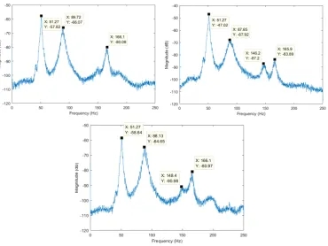
PSD plot. Then, instead of sending the whole FFT result, each sensor node only send FFT data corresponding to frequency location of obtained peaks. Using this method, it can be seen that the data transmission can be greatly reduced. However, each sensor could have different shape of PSD and natural frequency location. Figure 2.3 illustrate this.

Figure 2.3: PSD plot from three sensor used for pit bridge measurement

(18)

frequency points, it is still possible to obtain correct natural frequencies. This reduce the size of required FFT result data. If FFT operation is applied locally in each sensor node, this will effectively reduce the data transmission to central node. Based on this observation, a three phase distributed FDD is proposed. The details of each phase will be explained in following subsections. In order to explain the method easily, the same previous example, pit bridge measurement result, is used throughout the remaining explanations.

2.3.1 First Phase of Distributed FDD

[image:18.595.102.489.332.536.2]

The first phase objective is to find set of frequency points area to be used for finding true natural frequency locations in the second phase. For convenience purposes, this set of area is called peak areas. The complete process of first phase is illustrated in diagram on figure 2.4.

Figure 2.4: First Phase Process of Distributed FDD

(19)

[image:19.595.200.395.124.314.2]

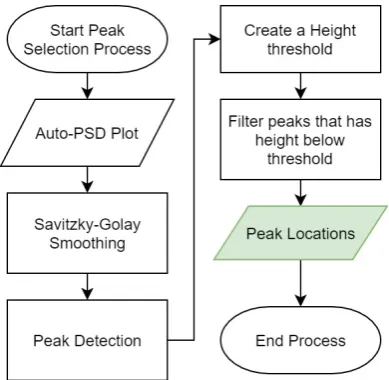
Figure 2.5: First Phase Peak Selection Process

The PSD plot is smoothed using Savitzky-Golay [21] smoothing filter first to reduce noises and jagged part of the plots. Savitzky-Golay is used as it can produce good smoothing while maintain peak shapes compared to simple moving average smoothing. The peak detection algorithm, based on the work of Yoder [22], is applied to the smoothed plot to obtain peak candidates. The algorithm is sufficiently reliable to detect peaks in noisy signal or plot. However, it is not perfect, there is still possibility that some noises or false positive are detected. Thus, additional process is added. Since, natural frequency peaks tend to be dominant height-wise, all of peak candidates are filtered based on their height. If the height is sufficiently high, it is passed. The height threshold is based on a percentage of the highest peak height. This thresholding result in set of peak locations that acts as potential natural frequency locations.

(20)

[image:20.595.119.479.157.513.2]

obtained. The process is best explained using example plot in figure 2.6.

Figure 2.6: First Phase Peak Area Construction Example from Two Sensors

(21)

2.3.2 Second Phase of Distributed FDD

[image:21.595.100.497.202.525.2]

The second phase objective is finding the true global natural frequencies using the FFT result data located in peak areas from first phase. The complete process of second phase is illustrated in figure 2.7.

Figure 2.7: Second Phase Process of Distributed FDD

(22)

overlapping is used for signal with sampling rate of 500 Hz, then each sig-nal window has time duration of 4.096 seconds. If user desire the minimum length of vibration signal is 204.8 seconds, then there will be 50 windows of signal needs to be processed. Thus, 50 times of process iteration needs to be done. Longer vibration signal acquisition will results in lower noise in resulted singular value plot from FDD process, which means lower chance of false positive in natural frequency detection. After sufficient iterations, sen-sor node will stop the process and idle wait further reply from central node. As can be observed, since commonly there are only so many peaks detected from previous phase and the peak area size limited, the data transmission is greatly reduced compared to sending the complete FFT result data.

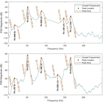
[image:22.595.108.489.532.659.2]

Upon receiving FFT data of whole iterations from all of the sensor node, cen-tral node will start the remaining FDD process to obtain modal parameters. All of the FFT result data are transformed into PSD matrix, one matrix for each peak area. The same FDD process as centralized one are applied. SVD is performed for each frequency points in the peak area, then singular value plot is constructed. The difference is in the peak selection. On normal centralized FDD, user need to select the peak manually. In this proposed solution, everything is done automatically, including the peak selection. The same peak selection process used in sensor node on first phase, illustrated in figure 2.6, is applied. The only difference is, instead of using PSD plot, it uses first singular value plot. After obtaining the peak locations, which corre-spond to natural frequencies, mode shapes are extracted from correcorre-sponding first singular vector. This process are done repeatedly until all of the peak areas are processed. The process and result can be further explained by example in figure 2.8.

(23)

Based on first phase result, there are five peak areas obtained, which their location in frequency points is shown as yellow line in figure 2.8. The blue line shows the frequency points where the FFT result data are discarded or not transmitted by sensor node. Since there are five peak areas, the modal parameter estimation process of central node is repeated five times, each iteration process different peak area. The example of smoothed singular value plot used in automatic peak selection is shown in right-side plot of figure 2.8. It can be noted that the first peak area is false positive. It is caused by at least one of the sensor detects local peak in auto-PSD plot around the area that does not correspond to the global natural frequency. However, by combining data from multiple sensor using SVD, the second phase process reliably determine that there is not any natural frequency peak located in the first peak area.

As mentioned previously, natural frequencies could be shifted due to various factors. As a consequence, peak areas are still needed to capture the correct modal parameters for next phase, as it is not possible to predict the natural frequency shift. Therefore, central node will make a new set of peak areas around the obtained natural frequencies, but using minimum area width. Since the frequency shift is commonly minimal, a narrow peak area such as 3 Hz is sufficient. Using example result in figure 2.8, there will be four peak areas, which are located in 50.039 53.039 Hz, 87.411 90.411 Hz, 147.010 -150.010 Hz, and 163.864 - 166.864 Hz. This new peak area information are sent back to all sensor node for next phase.

2.3.3 Third Phase of Distributed FDD

(24)

Figure 2.9: Third Phase Peak Selection Process

It starts with the same as subprocess as previous peak selection process, applying Savitzky-Golay smoothing to reduce noise peaks in first singular value plot. Then, peak location or natural frequency is obtained by simply finding the maximum value of smoothed singular value plot.

(25)

Experiment Result

In order to test the proposed distributed frequency domain decomposition, three operational modal analysis experiments are done in real bridge struc-ture located on the campus of University of Twente. The three experiment follows similar scenario. Six wireless inertial sensors, ProMove-Mini, pro-duced by Inertia Technology B.V. are used to measure the vibration of the bridge as acceleration under ambient excitation for a specific duration.

All of the bridge is measured using 500 Hz sampling rate to provide suf-ficiently broad frequency detection capability. The vibration measurement is done twice, so each bridge produce two set of vibrations data. The first vibration data is used for the first and second phase of distributed FDD and the other set of data is used for second phase. Each experiment uses 2048 point windowed FFT for their processes. Each window is filled fully with vibration signal, without zero-padding. Therefore, the FFT produces effec-tive frequency bin resolution of 0.244 Hz. The windowing function used is Hanning and PSD estimation is done without overlap between each window.

Four windows are used to estimate auto-PSD in first phase of each experiment setup. Regarding PSD and singular plot smoothing, Savitzky-Golay filter with order of 3 and length of 13 data points is used for all experiments to make sure a good trade-off between smoothing and peak shape preservation. In order to separate the natural frequency peaks from insignificant false positive peaks, peak height threshold for all peak selection process in each of the experiments is set to 30 percents of highest peak height. Peak area width of second phase and third phase for all experiment are set to 15.6224 Hz (65 frequency bins) and 2.9311 Hz (13 frequency bins) respectively.

(26)

3.1 Pit Bridge

The first experiment is performed in a small pit bridge located in University of Twente. The construction of the bridge can be seen in figure 3.1. The bridge has width of 169.2 cm and length of 106 cm. The structure is made of steel with steel mesh deck.

Figure 3.1: The structure of the pit bridge of University of Twente

The six sensor are placed on top of deck with arrangement that follows fig-ure 3.2.

Figure 3.2: Sensor placement on the pit bridge of University of Twente

(27)

which produces 118784 samples each. The example of acquired vibration signal is shown in figure 3.3.

Figure 3.3: Vibration Signal Example of Pit Bridge Measurement

The vibration signal is processed with 58 windows of 2048 point FFT to obtain PSD matrix for second and third phase. Processing the obtained data using first phase and second phase distributed produce result as shown in figure 3.4.

Figure 3.4: Second Phase Result Plot of Pit Bridge Experiment

(28)

[image:28.595.136.460.409.686.2]

to determine that there is not any natural frequency in that peak area. As can be seen from the plot as well, not all frequency points are necessary to perform obtain the natural frequency. Therefore, there are already some data transmission reduction from second phase. Using natural frequency results obtained from second phase, a third phase distributed FDD is performed. The resulted modal parameters and its comparison to second phase result is summarized in table 3.1.

Table 3.1: Third Phase Result of Pit Bridge Experiment

Third Phase Natural Frequency (Hz)

Second Phase Natural Frequency (Hz)

Natural Frequency Difference (%)

MAC Value Third Phase vs

Second Phase

51.050 51.539 0.948 0.991

87.934 88.911 1.099 0.973

148.754 148.510 0.164 0.976

165.608 165.364 0.148 0.995

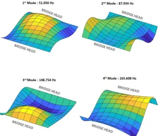
Resulted mode shapes are illustrated in the figure 3.5.

(29)

The result shows that the natural frequency difference between second phase and third phase is minuscule. The resulted mode shape also have good and unique shape. The high MAC values for all mode shapes shows that third phase produce consistent mode shape. These results also signifies that all of the peaks detected are true modal peaks, since they produce consistent result between two separate measurements. In order to find out how well the performance of this distributed FDD compared to normal centralized FDD, a further comparison result are made. The centralized FDD is performed by simply follow the normal FDD process and selecting peaks by manually select the highest value of peaks on the singular value plots. Obtained result is shown in table 3.2.

Table 3.2: Centralized FDD Comparison Result of Pit Bridge Experiment

Third Phase Natural Frequency (Hz) Centralized FDD Natural Frequency (Hz) Natural Frequency Difference (%) MAC Value Third Phase vs Centralized FDD

51.050 51.050 0.000 1.000 87.934 87.934 0.000 1.000 148.754 148.754 0.000 1.000 165.608 165.852 0.147 0.998

The comparison results shows that except fourth mode, all of the third phase modal parameters are same as centralized FDD result. The highest frequency difference is only 0.147 percent and the lowest MAC value is still quite high, which is 0.998. Regarding the data size reduction, the table 3.3 summarized them.

Table 3.3: Data Size Comparison of Pit Bridge Experiment

Data Name Data Type Data Type Size (byte) Number of Data Total Data Size (byte) Data Saving Compared To Time Domain Signal (%)

Time Domain Signal Float 4 118784 475136 -Second Phase

FFT Result (58 Windows)

Complex Float 8 408 189312 60.16

Third Phase FFT Result (58 Windows, 4 peaks)

Complex Float 8 754 6032 98.73

(30)

comparison. The result in table 3.3 assumes that time domain signal is always represented by 32-bit floating point. The FFT result always produce complex number that represented in 32-bit floating point number. Since each complex number consist of two part, imaginary and real number, each data has twice the size of 32-bit floating point number. The data size for second phase and third phase is sum of 58 windows of FFT result data. Third phase data size is also the sum of four peaks, where each peak area consist of 13 frequency bins. The result shows that second phase reduce the data size needed to determine initial natural frequencies quite significantly. Third phase reduce it even further until the data size is only 1.27 percents of original time domain signal data size.

3.2 Steel Arch Bridge

The second experiment is performed on a pedestrian steel arch bridge located in University of Twente campus. The structure of the bridge can be seen in figure 3.6. The structure itself contain two identical bridge (left and right) that does not have any connection to each other. Each part of the bridge has arc length of 499 cm and width 99.6 cm. The deck of the bridge has similar shape as previous pit bridge, comprises of steel meshes.

Figure 3.6: The structure of the steel arch bridge of University of Twente

(31)

[image:31.595.105.487.329.529.2]

Figure 3.7: Sensor placement on steel arch bridge of University of Twente

All of the sensors are placed by tightly strap them into the mesh structure of bridge deck. The detailed sensor placement diagram can be seen in figure 3.8.

Figure 3.8: Detailed sensor placement diagram on steel arch bridge

(32)

Figure 3.9: Vibration Signal Example of Steel Arch Bridge Measurement

Processing the obtained data using first phase and second phase distributed produce result as shown in figure 3.10.

Figure 3.10: Second Phase Result Plot of Steel Arch Bridge Experiment

(33)

As a consequences, higher chance of false positive will occurs. Using natural frequency results obtained from second phase, a third phase distributed FDD is performed. The resulted modal parameters and its comparison to second phase result is summarized in table 3.4.

Table 3.4: Third Phase Result of Steel Arch Bridge Experiment

Second Phase

20.762 20.762 0.000 0.985

24.670 24.670 0.000 0.966

27.113 27.601 1.770 0.990

43.967 44.211 0.552 0.888

77.675 76.698 1.274 0.969

(34)

[image:34.595.127.465.129.520.2]

Figure 3.11: Mode Shapes of Steel Arch Bridge Experiment

(35)

bridge, the potential movement on that part cannot be shown in obtained mode shapes.

Figure 3.12: Railing Connection on Steel Arch Bridge Experiment

[image:35.595.180.414.168.346.2]

A further comparison result between third phase and normal centralized FDD is also made. The comparison result is shown in table 3.5.

Table 3.5: Centralized FDD Comparison Result of Steel Arch Bridge Exper-iment

Centralized FDD Natural Frequency (Hz)

MAC Value Third Phase vs Centralized FDD

20.762 20.762 0.000 1.000 24.670 24.670 0.000 1.000 27.113 27.113 0.000 1.000 43.967 43.967 0.000 1.000 77.675 78.652 1.242 0.980

(36)

[image:36.595.101.494.150.272.2]

Table 3.6: Data Size Comparison of Steel Arch Bridge Experiment

Data Name Data Type Data Type Size (byte)

Number of Data

Total Data Size (byte)

Data Saving Compared To Time Domain Signal (%)

Complex Float 8 26230 209840 70.21

Complex Float 8 1118 8944 98.73

The data size reduction is shown in table 3.6. The result shows that second phase reduce the data size significantly. As same as result in pit bridge experiment, third phase reduce it even further until the data size is only 1.27 percents of original time domain signal data size.

3.3 Wood Arch Bridge

The third experiment is performed on an arch bridge with wood structure, except the deck, which is made up of multiple beams of asphalt. This bridge is larger than two previous bridge, with the arc length of 12.9 m and width of 2.1 m. The photos of the structure can be seen in figure 3.13.

Figure 3.13: Wood arch bridge of University of Twente

[image:36.595.103.492.473.583.2]

(37)

[image:37.595.200.396.127.273.2]

Figure 3.14: Sensor placed on top of Wood Arch Bridge

Figure 3.15: Diagram of sensor placement in Wood Arch Bridge

[image:37.595.106.464.328.524.2]

(38)

[image:38.595.129.461.135.293.2]

Figure 3.16: Vibration Signal Example of Wood Arch Bridge Measurement

[image:38.595.109.488.408.588.2]

PSD matrix for second and third phase are estimated using 42 windows of 2048 point FFT. Processing the obtained data using first phase and second phase distributed produce result as shown in figure 3.17.

Figure 3.17: Second Phase Result Plot of Wood Arch Bridge Experiment

(39)

[image:39.595.120.467.179.345.2]

on second dataset (used for third phase), those two peaks also apparent, albeit weaker, as shown in figure 3.18.

Figure 3.18: Missed Natural Frequency Peaks on Wood Arch Bridge Exper-iment. Peaks in singular value plot of first dataset (left) and second dataset (right)

Checking the mode shape of those peaks between two dataset result also shows that they correlate well, with MAC value of 0.9898 and 0.9115 re-spectively. This signifies that they are true modal peak. This problem is caused by the smoothing procedure in first phase and second phase. Those two peaks are suppressed by the smoothing procedure as they are narrow peaks with small height. Reducing the smoothing intensity could increase the possibility of those two peaks detected. However, it also increases the possibility of false-positive peak detection as the singular value plot is quite noisy. This noisy plot is caused by insufficient duration of signal acquisition. As can be noted, the wood arch bridge experiment has the shortest vibration acquisition duration. By increasing the vibration signal length, noise can be further suppressed and natural frequency peak becomes more apparent, which result in more reliable peak selection process.

(40)

[image:40.595.101.493.152.246.2]

Table 3.7: Third Phase Result Wood Arch Bridge Experiment

Second Phase

8.061 8.305 2.941 0.965

16.854 16.854 0.000 0.997

20.029 20.274 1.205 0.957

52.272 53.004 1.382 0.911

Resulted mode shapes illustration is shown in figure 3.19.

Figure 3.19: Mode Shapes of Steel Arch Bridge Experiment

[image:40.595.113.476.307.589.2]

(41)

two measurements. This is further proofed by the fact that all of the mode shapes are unique.

A further comparison result between third phase and normal centralized FDD is performed to see how accurate is the proposed distributed FDD. The com-parison result is shown in table 3.8.

Table 3.8: Centralized FDD Comparison Result of Wood Arch Bridge Ex-periment Third Phase Natural Frequency (Hz) Centralized FDD Natural Frequency (Hz) Natural Frequency Difference (%) MAC Value Third Phase vs Centralized FDD

8.061 8.061 0.000 1.000 16.854 16.610 1.471 0.995 20.029 20.029 0.000 1.000 52.272 52.272 0.000 1.000

The comparison results shows that all of the modal parameters resulted in third phase are consistent with centralized FDD. Three of the modal param-eters are as same as centralized FDD result. The one that is sightly differ, third mode, even shows high MAC value and minuscule natural frequency difference.

Table 3.9: Data Size Comparison of Steel Arch Bridge Experiment

Data Name Data Type Data Type Size (byte) Number of Data Total Data Size (byte) Data Saving Compared To Time Domain Signal (%)

Complex Float 8 10500 84000 75.59

Complex Float 8 546 4368 98.73

(42)

Practical Review

In order to asses the feasibility of the proposed distributed FDD to be imple-mented in resource constrained wireless sensor node, a resource usage analysis are performed. There are four main aspect that will be reviewed, which are processing power, memory usage, data transmission, and battery usage. In order to review the each of the resource usage, distributed processes of sensor node side are implemented in real microcontroller.

Since the nature of proposed distributed FDD involves lot of floating point computation and deals with huge data in sensor node side, it is desirable to use microcontroller that has floating point unit and large size of Ran-dom Access Memory (RAM). Based on this, STM32F407VG microcontroller made by ST Microelectronic, is chosen for the implementation. It has popu-lar 32-bit ARM Cortex-M4 processor that include floating point unit in the architecture. It also has 192 Kilobytes of RAM, which fits perfectly with the requirement, and 1 Megabytes of Flash memory that could fit large appli-cation in it. Moreover, the microcontroller supports operating frequency of 168 MHz, which provides high computational speed capability.

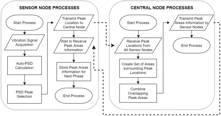
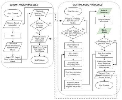
The complete process implementation for all phases of distributed FDD on the microcontroller is illustrated in the figure 4.1. Important thing to take note is that there is not any complementary hardware used, such as real accelerometer and radio hardware used for the implementation. The imple-mentation only focused on microcontroller side. Thus, some process part are not fully implemented.

(43)

[image:43.595.102.490.102.346.2]

Figure 4.1: Process Diagram of Distributed Processes in Sensor Node Side

The diagram also explain which path of processes are taken for each phase of distributed FDD. The explanation for each process part as follows:

• Initialization is used for setting up external peripherals or hardware such as accelerometer and radio module. However, since there is not any external hardware used, this part of process is left empty and do nothing.

• Signal Acquisitonis the process where data is polled from accelerom-eter and arranged to be saved for further processing. However, this process is partially implemented since there is not any real accelerom-eter used. The data saving process is as same as the case when real accelerometer data is used. The difference is in data polling, where a dummy process is used to poll testing data. Despite that, the differ-ence to real accelerometer data poling is expected to be minimal, since commonly accelerometer use fast SPI communication to transfer data to microcontroller. Signal acquisition is stopped when certain number of samples are already polled. In the previous experiment case, it is the length of signald window needed for FFT, which is 2048 samples.

(44)

FFT process. A library provided by ARM called CMSIS-DSP is used for implementing the FFT.

• FFT Data Selection is process of selecting FFT result data that needs to be sent based on obtained peak area from phase 1 and phase 2.

• FFT Data Payload Construction is process of constructing packet data payload that will be sent via radio transmission to central node. This process involves creating header, splitting data into set of packets, and arranging data in packet payload.

• PSD Calculation is process of creating auto power spectral density plot in the first phase to determine peak location candidate for peak area construction. This process also involves multiple windowed FFT calculation similar to FFT calculation process part mentioned previ-ously.

• PSD Peak Calculation is process to be run on the first phase for determining the peak locations in PSD plot.

• Packet Transmission is process where microcontroller instruct the radio hardware to send required data. This process is not different for each type of payload needed to be sent. Since there is not any real radio hardware used, this process is not implemented. It is expected that this process execution time is very short such that it is insignificant, since it only involves fast microcontroller to radio module communication.

• Command Packet Receptionis process where microcontroller check and communicate with radio hardware for incoming packet from cen-tral node. Due to similar reason as Packet Transmission process, this process is not implemented and it is expected that the execution time is insignificant.

• Command Packet Handleris a process where received packets from central node are processed into set of meaningful data that will be saved for further processing. The kind of data involves are instruction to start first phase, and peak area information result from second and third phase. This process is fully implemented and tested using fake packet data that replicates real command packets.

(45)

and computational register values are erased while microcontroller is in deep sleep mode. Therefore, an important data backup mechanism to permanent memory (such as flash) or backup SRAM (STM32F407VG have one) are performed before sleeping. Aside of that, the common operation involves setting up some microcontroller registers and real time clock. This process is not implemented and it is expected that the execution time is minuscule since the heaviest operation is only fast copying data from register or RAM to another memory location.

The clock speed of microcontroller is set to 168 MHz. All of the processes are written in a application that is run directly on top of STM32F407VG without any medium layer between such as operating system. The application is compiled by open source ARM-GCC compiler using O2 optimization flag. Each resource usage analysis is explained further in following subsections.

4.1 Processing Power

The metric that will be used to see how much the processing power toll on wireless sensor node is processing time. The longer processing time required to compute complete processes of each phases of proposed distributed FDD, the higher power consumption for microcontroller usage. If the processes are too heavy and takes very long time to finish, it is possible that the power consumption for computation is similar to or more than the power used for data transmission, which could defeat the purpose of data reduction on distributed process.

(46)

[image:46.595.99.496.150.295.2]

Table 4.1: First Phase Processes Execution Time

First Phase Process

Pit Bridge Total Process Execution Time (µs)

Steel Bridge Total Process Execution Time (µs)

Wood Bridge Total Process Execution Time (µs)

Signal

Acquisiton 27.95 27.96 27.93

PSD

Calculation 98780.00 98788.00 98856.00

PSD Peak

Detection 1461.60 1465.10 1458.80

Peak Data

Payload Construction 0.29 0.29 0.29

Command

[image:46.595.103.493.338.483.2]

Packet Handler 1.28 1.28 1.27

Table 4.2: Second Phase Processes Execution Time

Second Phase Process

Signal

Acquisition 402.26 596.63 291.34

FFT

Calculation 68005.00 100835.00 49245.00

FFT Data

Selection 1194.05 1770.40 700.01

FFT Data

Payload Construction 4409.04 6537.72 2528.57 Command

Packet Handler 83.20 123.37 59.72

Table 4.3: Third Phase Processes Execution Time

Third Phase Process

Signal

Acquisition 402.39 596.69 291.40

FFT

Calculation 68005.00 100835.00 49245.00

FFT Data

Selection 420.33 623.41 251.80

FFT Data

Payload Construction 1278.44 1895.53 713.79 Command

Packet Handler 53.17 78.84 38.50

[image:46.595.103.493.525.672.2]

(47)

experiment scenario, where the highest number of vibration signal windows (86 windows) are applied by windowed FFT. However, the execution only requires 100.835 milliseconds. The total execution time for all of the phase, in all of the bridge experiments, are below than 1 second. In this case, micro-controller spend more time idle waiting for accelerometer data, which can be batch polled, or idle waiting command packet from central node than process-ing the vibration signals. In both case, microcontroller can be put in lower energy consumption mode. Therefore, processing power is not a problem for sensor node development, seeing there are lot of cheap microcontroller with ARM Cortex-M4 processor aside of STM32F407VG. Of course the execution time can be increased if user set the required vibration signal duration to be longer, which means higher number of phase 2 and phase 3 process iteration. However, the total execution is very small such that even though the length is increased to 100 times longer, the required total execution time for each phase is still in unit of seconds.

4.2 Memory Usage

(48)

[image:48.595.102.494.150.310.2]

Table 4.4: RAM Usage Detail

Data Name Data Type Type Size (Bytes)

Number of Data

Total Data Size (Bytes)

Vibration Signal Float 4 2048 8192 Auto PSD Data Float 4 1024 4096 Peak Locations Integer 16-bit 2 20 40 FFT Result Data Complex Float 8 1024 8192 Peak Area Location Indices 2 x Integer 16-bit 4 20 80 Number of Iteration Integer 16-bit 2 1 2

Stack Size - - - 4096

Others - - - 986

Total RAM Usage

25684

Vibration Signal is used to store acquired vibration from accelerometer, it holds 2048 samples of data, which is equal to the window size for FFT and PSD calculation. Auto PSD Data holds the auto-PSD result calculation. Since auto-PSD always produces real result and half of the frequency points are unused, it is sufficient to hold only 1024 samples of floating point number. FFT result data contains data resulted from FFT operation of all of the distributed FDD phases. Peak locations are used to store the location of peak obtained from first phase. Peak area location indices is used to store information about peak areas obtained from central node as a result of second and third phase. Each of its data contain one number that signifies in which location the peak area start, and one number that signifies where the peak area should end. Both Peak Area Location Indices and Peak Locations are set to contain a fixed number of data, up to maximum 20 data. Number of Iteration store the information from central node about how many process iteration needed to finish second or third phase. This number of iteration correspond to the length of vibration signal that is needed to be processed for complete modal analysis in second or third phase. In microcontroller, stack size should be set manually to a fixed size. Understanding that some of the functions involve large data operation, in order to avoid stack overflow, it is set to 4096 bytes. There are some others data that uses 986 bytes which cannot be tracked, this could consists of global variables from external libraries or board and processor startup routine.

(49)

based microcontroller. Microcontroller that uses ARM Cortex-M4 processor often includes large RAM in it. To give some example, NRF52 from Nordic Semiconductor has 64 kilobytes of RAM and SAM4S from Atmel provides 160 kilobytes of RAM.

One thing to take a note is that the RAM usage is independent from the required length of vibration signal. Previous Wood Arch Bridge experiment, that involves vibration signal length of 172.032 seconds (42 windows of 2048 samples) use the same RAM size as Pit Bridge experiment that uses 352.26 second long of vibration signal (86 windows of 2048 samples). No matter how long the required signal duration to be processed, they basically use the same set of processes and data storage over and over again for each windows until sufficient number of windows processed. Each iteration, the old data is replaced by newly produced data as it no longer serves any use. However, the RAM usage can be changed if different number of point of FFT used. In current experiments case, 2048-point FFT is used. If it changed into 4096-point FFT, the RAM usage could increase to almost twice the size of RAM usage in 2048-point FFT scenario. Therefore, it is advisable to use as minimum number of point of FFT as possible, as long as it meets the frequency resolution requirements.

4.3 Data Transmission

The data reduction comparison that has been shown in previous chapter il-lustrates how significant the proposed distributed FDD able to reduce the data needs to be transmitted. However, in real practice, the data transmis-sion will always be larger. This is due to packet header and payload size limitation for single packet transmission. Both of them are unique to the communication protocol and the radio hardware being used. Thus, in order review the practicality of proposed distributed FDD from data transmission perspective, a specific radio hardware should be selected for hypothetical testing scenario.

(50)

a good protocol candidate to be used in real application. It has high data rate, typically 250 kilobits per-second (31.25 kBps). It can cover large area by utilizing its capability to construct a mesh network. Therefore, ZigBee is used for data transmission review. A popular ZigBee radio module, Xbee ZB is chosen. It has maximum outdoor range capability of 120 m and indoor range of 40 m in single hop.

[image:50.595.105.493.474.642.2]

Xbee ZB have payload size limitation of 84 bytes for each packet. It also needs a 13 byte headers for ZigBee protocol. Another 3 byte custom header is needed for distributed FDD usage. The first byte signifies what type of packet is transmitted or received, second byte signifies the total number of packets is sent in current communication session, and third byte signifies the packet number. Last two bytes are used in case transmitted data are splitted into multiple packets. Using these two bytes, central node can track the order of packets and easily merge the them into one single set of data again. As can be observed, the data transmission size tends to be larger, especially on FFT result data. Payload size limitation force the FFT result data to be splitted into multiple packet. Each packet contain its own header. The resulted final transmission size are shown in table 4.5 for Pit Bridge experiment, table 4.6 for Steel Arch Bridge experiment, and table 4.7 for Wood Arch Bridge experiment. The original data size is based on previous chapter experiment results.

Table 4.5: Data Transmission Details for Pit Bridge experiment

Packet Type Data Size (bytes) Header Size (bytes) Number Of Packet Total Transmission Size (bytes) Transmission Duration (ms) First Phase

Peak Locations 10 16 1 26 0.80 Second Phase

FFT Data 189312 16 2254 225360 6935.38 Second Phase

Peak Areas 20 16 1 36 1.11 Third Phase

FFT Data 6032 16 72 7168 221.54 Third Phase

(51)

[image:51.595.104.493.149.318.2]

Table 4.6: Data Transmission Details for Steel Arch Bridge experiment

Peak Areas 20 16 1 36 1.11

Table 4.7: Data Transmission Details for Wood Arch Bridge experiment

Peak Areas 16 16 1 32 0.98

[image:51.595.105.493.366.535.2]

(52)

is very low such that battery life can be preserved well. How long a battery life preserve will be further explained in next section.

4.4 Energy Consumption

Mainly there are three main energy consumer in sensor node, which are mi-crocontroller, radio module, and accelerometer (or other vibrational sensor). In some cases, external real time clock is used to schedule sleep and wake up. However, STM32F407VG has internal RTC to support its energy sav-ing mode. As same as other resource usage review, it is needed to make a use case using real hardware data, as without it is not possible to estimate energy consumption. Microcontroller and radio module hardware choice is already clear. For convenience purpose, a popular digital output accelerom-eter, LIS3DH, made by STMicroelectronics is used for energy consumption review. Using datasheet of each hardware, a summary of current consump-tion is shown in table 4.8.

Table 4.8: Current Consumption Summary of Main Hardware

Hardware State Current Consumption (mA)

Microcontroller

Active 87

Microcontroller Sleep 0.0003 Radio Transmit 45 Radio Receive 40 Radio Sleep 0.001 Accelerometer Active 0.011 Accelerometer Sleep 0.0005

(53)

[image:53.595.107.493.149.327.2]

Table 4.9: Current Consumption Details of First Phase Hardware State on First Phase Pit Bridge Experiment Steel Bridge Experiment Wooden Bridge Experiment Duty Cycle (%) Effective Current Consumption

(µA)

Duty Cycle (%)

Effective Current Consumption

(µA)

Duty Cycle (%)

(µA) Microcontroller

Active 0.0028 2.42 0.0028 2.42 0.0028 2.42

Microcontroller

Sleep 99.9972 0.30 99.9972 0.30 99.9972 0.30

Radio Transmit 0.0007 0.30 0.0007 0.30 0.0007 0.30

Radio Receive 0.0009 0.37 0.0007 0.29 0.0007 0.29

Radio Sleep 99.9984 1.00 99.9986 1.00 99.9986 1.00

Accelerometer

Active 0.4551 0.05 0.4551 0.05 0.4551 0.05

Accelerometer

Sleep 99.5449 0.50 99.5449 0.50 99.5449 0.50

Total 4.94 Total 4.86 Total 4.86

Table 4.10: Current Consumption Details of Second Phase

Hardware State on Second Phase Pit Bridge Experiment Steel Bridge Experiment Wooden Bridge Experiment Duty Cycle (%) Effective Current Consumption

(µA)

Duty Cycle (%)

(µA)

Duty Cycle (%)

Active 0.0021 1.79 0.0031 2.66 0.0015 1.28

Microcontroller

Sleep 99.9979 0.30 99.9969 0.30 99.9985 0.30

Radio Transmit 5.7785 2600.31 6.4053 2882.40 2.5641 1153.85

Radio Receive 0.0008 0.33 0.0009 0.37 0.0008 0.33

Radio Sleep 94.2207 0.94 93.5937 0.94 97.4351 0.97

Accelerometer

Active 6.5991 0.73 9.7849 1.08 4.7787 0.53

Accelerometer

Sleep 93.4009 0.47 90.2151 0.45 95.2213 0.48

[image:53.595.106.493.376.556.2]

(54)

Table 4.11: Current Consumption Details of Third Phase Hardware State on Third Phase Pit Bridge Experiment Steel Bridge Experiment Wooden Bridge Experiment Duty Cycle (%) Effective Current Consumption

(µA)

Duty Cycle (%)

(µA)

Duty Cycle (%)

Active 0.0019 1.70 0.0019 1.70 0.0014 1.22

Microcontroller

Sleep 99.9981 0.30 99.9981 0.30 99.9986 0.30

Radio Transmit 0.1838 82.71 0.2728 122.77 0.1333 60.00

Radio Receive 0.0008 0.33 0.0008 0.33 0.0008 0.33

Radio Sleep 99.8154 1.00 99.7264 1.00 99.8658 1.00

Accelerometer

Active 6.5991 0.73 9.7849 1.08 4.7787 0.53

Accelerometer

Sleep 93.4009 0.47 90.2151 0.45 95.2213 0.48

Total 87.22 Total 127.62 Total 63.85

Since there is a possibility of using multihop transmission in ZigBee and pos-sibility of transmission loss, the radio transmit and receive state is modified for all of the phases. The original transmission and reception duration shown in previous section is multiplied by 30 to accommodate the possibility of us-ing 5 hops with 6 times retransmission for each hop for worst case scenario when there are multiple packet loss. Current consumption data from all of the phases shows that the dominant energy consumer is indeed the wireless communication.

Based the total effective current consumption of all of the phases in tables above, battery life in hours can be estimated using following formula:

BatteryLif e= Ebatt×ηbatt−itphase1−itphase2

itphase3

(4.1)

where Ebatt is battery capacity (in mAh), ηbatt is battery efficiency (in per-cent), itphase1 is total effective current consumption of first phase (in mA),

itphase2 is total effective current consumption of second phase (in mA), and

itphase3 is total effective current consumption of third phase (in mA).

(55)

Conclusion and Recommendation

5.1 Conclusion

In this thesis, a distributed Operational Modal Analysis for wireless sensor network has been designed. It is based on Frequency Domain Decomposition (FDD) algorithm. However, instead of applying FDD to the full frequency points (half of the sampling rate), the FDD is applied only to small frequency point area around natural frequencies. By performing FFT operation part of FDD locally in sensor node, data transmission size could be reduced sig-nificantly.

Operational modal analysis experiment on three real bridge is performed to assess the capability of the proposed distributed FDD. Overall, the result shows that it can reliably automatically extract true modal parameters out of vibration signal data, except on one occasion. In one of the bridge ex-periment, the process missed two out six modal parameters. The result also shows the size of data that needs to be transmitted from sensor node is re-duced significantly, with size of only 1.27 percents of the raw time-domain vibration signal.

Moreover, practical feasibility review is also performed by implementing the process on real microcontroller, an ARM-Cortex M4 based STM32F407VG. Hypothetical hardware usage scenario is also used to inspect the resource usage further. The wireless communication is assumed to be performed via ZigBee protocol using Xbee ZB radio, and vibration signal is acquired via LIS3DH accelerometer. The result shows that all of the processes are exe-cuted quickly on the sensor node, with the highest execution time of 100.835 ms. The total RAM usage of 25.684 kilobytes also fits within the microcon-troller RAM size and expected to be fit with other ARM-Cortex M4 based

(56)

microcontrollers. The energy consumption estimation , based on the all of the bridge experiment usage scenario, shows that sensor node lifetime could exceed one year using only 2000 mAh battery.

In conclusion, the proposed distributed FDD shows good promise for real wireless sensor network implementation as it can automatically and reliably detect modal parameters from real data while using minimum resources on wireless sensor node.

5.2 Recommendation

However, there are still some limitation on the process. Some of the process parameters are still set manually, especially in the peaks location and peak area selection. It is desirable if smoothing strength could be adapted auto-matically based on the intensity of noise in PSD plot or First Singular Value plot. If this can be applied, the smoothing process could produce higher qual-ity of plot and reduce the possibilqual-ity of false negative or false positive peak detection. A noise intensity metric based on the amount of local maxima and minima could be developed to pursue this.

Furthermore, current peak area is set into fixed width for all natural frequen-cies. This width could be unnecessarily too large. Width that is too large for frequency peaks that is closely spaced neighboring frequency peak will poten-tially produce erroneous result. The automatic peak selection could falsely select the neighboring natural frequency instead, if it is more dominant than the correct natural frequency. The peak area width should be adapted based on percentage of each natural frequency peak width itself.

(57)

References

[1] Scott W Doebling, Charles R Farrar, Michael B Prime, and Daniel W Shevitz. Damage identification and health monitoring of structural and mechanical systems from changes in their vibration characteristics: a literature review. 1996.

[2] Wei Fan and Pizhong Qiao. Vibration-based damage identification meth-ods: a review and comparative study. Structural Health Monitoring, 10(1):83–111, 2011.

[3] Peter C Chang, Alison Flatau, and SC Liu. Review paper: health moni-toring of civil infrastructure. Structural health monitoring, 2(3):257–267, 2003.

[4] MM Abdel Wahab and Guido De Roeck. Damage detection in bridges using modal curvatures: application to a real damage scenario. Journal of Sound and vibration, 226(2):217–235, 1999.

[5] Kai-Chun Chang and Chul-Woo Kim. Modal-parameter identification and vibration-based damage detection of a damaged steel truss bridge.

Engineering Structures, 122:156–173, 2016.

[6] Charles R Farrar and David A Jauregui. Comparative study of damage identification algorithms applied to a bridge: Ii. numerical study. Smart materials and structures, 7(5):720, 1998.

[7] Peter Van Overschee and Bart De Moor. Subspace algorithms for the stochastic identification problem. Automatica, 29(3):649–660, 1993.

[8] Soojin Cho, Jong-Woong Park, and Sung-Han Sim. Decentralized sys-tem identification using stochastic subspace identification for wireless sensor networks. Sensors, 15(4):8131–8145, 2015.

(58)

[9] Sung-Han Sim, BF Spencer, M Zhang, and H Xie. Automated decentral-ized modal analysis using smart sensors. Structural Control and Health Monitoring, 17(8):872–894, 2010.

[10] Rune Brincker, Lingmi Zhang, and P Andersen. Modal identification from ambient responses using frequency domain decomposition. InProc. of the 18*‘International Modal Analysis Conference (IMAC), San An-tonio, Texas, 2000.

[11] Julius S Bendat and Allan G Piersol. Engineering applications of corre-lation and spectral analysis. New York, Wiley-Interscience, 1980. 315 p., 1980.

[12] Jin-Hak Yi and Chung-Bang Yun. Comparative study on modal identi-fication methods using output-only information. Structural Engineering and Mechanics, 17(3 4):445–466, 2004.

[13] Bart Peeters and Guido De Roeck. Stochastic system identification for operational modal analysis: a review. Journal of Dynamic Systems, Measurement, and Control, 123(4):659–667, 2001.

[14] Randall J Allemang and David L Brown. A correlation coefficient for modal vector analysis. In Proceedings of the 1st international modal analysis conference, volume 1, pages 110–116. Orlando: Union College Press, 1982.

[15] A Cunha, Elsa Caetano, Rune Brincker, and Palle Andersen. Identi-fication from the natural response of vasco da gama bridge. In XXII International Modal Analysis Conference, 2004.

[16] Jian-Huang Weng, Chin-Hsiung Loh, Jerome P Lynch, Kung-Chun Lu, Pei-Yang Lin, and Yang Wang. Output-only modal identification of a cable-stayed bridge using wireless monitoring systems. Engineering Structures, 30(7):1820–1830, 2008.

[17] AT Zimmerman, RA Swartz, and JP Lynch. Automated identification of modal properties in a steel bridge instrumented with a dense wire-less sensor network. Bridge Maintenance, Safety Management, Health Monitoring and Informatics, pages 1608–1615, 2008.

(59)

[19] Gregory Hackmann, Weijun Guo, Guirong Yan, Zhuoxiong Sun, Chenyang Lu, and Shirley Dyke. Cyber-physical codesign of distributed structural health monitoring with wireless sensor networks.IEEE Trans-actions on Parallel and Distributed Systems, 25(1):63–72, 2014.

[20] Peter Welch. The use of fast fourier transform for the estimation of power spectra: a method based on time averaging over short, modi-fied periodograms. IEEE Transactions on audio and electroacoustics, 15(2):70–73, 1967.

[21] Abraham Savitzky and Marcel JE Golay. Smoothing and differentiation of data by simplified least squares procedures. Analytical chemistry, 36(8):1627–1639, 1964.

Distributed Processing for Operational Modal Analysis of Bridge Infrastructures Using Wireless Sensor Networks

Master Thesis