Facial feature processing using artificial neural networks

(1)

University of Warwick institutional repository:

http://go.warwick.ac.uk/wrap

A Thesis Submitted for the Degree of PhD at the University of Warwick

http://go.warwick.ac.uk/wrap/59539

This thesis is made available online and is protected by original copyright.

Please scroll down to view the document itself.

(2)

Facial Feature Processing

Using Artificial Neural Networks

Nicholas David Porter

A dissertation submitted in satisfaction of the requirements for

the degree of Doctor of Philosophy

University of Warwick

Department of Engineering

(3)

72

76 76 76 77 79 81 83 86 90 90 97

102

104

104

105 110 113 113 114 122

127

129

130

3.6

4 Experimental Data, Pre-processing and Analysis

4.1 The Data . . . . 4.1.1 The descriptive measures 4.1.2 Data acquisition

4.2 Pre-processing ...

4.2.1 Colour representations 4.2.2 Image segmentation 4.3 Data sets used

4.4 Data analysis

4.4.1 Principal Components Analysis. 4.4.2 Unsupervised Neural network methods.

5 Simple Feature Classification

5.1 Experimental Method ... 5.1.1 Statistical classifiers 5.1.2 MLP Networks ...

5.1.3 Radial Basis Function networks 5.2 Results...

5.2.1 Moustache classification 5.2.2 Beard classification. 5.3 Conclusions...

6 More Complex Feature Classification

6.1 Experimental Method ...

(6)

CONTENTS

6.1.1 Statistical Classifiers . . . . 6.1.2 Neural Network Classifiers. 6.2 Results...

6.2.1 Statistical Classifiers 6.2.2 Neural Network Classifiers. 6.3 Further Neural Network Methods .

6.3.1 Experimental Methods.

6.3.2 Results .

6.3.3 Combining the networks

6.3.4 Comparing the classification methods 6.4 Further Data Analysis

6.5 Conclusions .

130 131 134 134 139 151 151 153 155 159 161 163

7 Conclusions

7.1 Future Work

166

168

A Derivation of

f'

172

B Conversion of RGB colour values to other representations

C Graphs Used in Evaluating Training Parameters

175

177

194

D Publication from work in this thesis

References 199

209

Bibliography

(7)

Abbreviations and Symbols

Mathematical conventions

The following conventions have been adopted for the presentation of mathematical information within this thesis:

X The variablex.

x The vector x.

Xi The ith element of vector x.

xT The transpose of the vector x.

X The matrix X.

Xj The j row of the matrix X.

Xji The element at the jth row and ith column of matrix X.

In some instances the row and column indices for matrices are reversed. This is made clear by the definitions in the relevant sections:

Abbreviations

The followingis a list of the abbreviations and symbols used in this thesis along with their meaning.

a Activation: the result of the weighted sum of inputs to a neuron. ANN Artificial Neural Network.

Cl! Learning rate.

bpp Bits per pixel.

(8)

ABBREVIATIONS AND SYMBOLS

CMY The cyan, magenta, yellow colour encodingscheme,

CMYK The cyan, magenta, yellow, black colour encoding scheme.

E Network error.

E;

Error from node i.

Ep Network error with pattern p on the inputs.

f

0

A network transfer function, usually sigmoidal.

GA Genetic Algorithm

HSV The hue, saturation, value colour encoding scheme. MLP Multilayer Perceptron.

r The learning signal in the general learning rule (see 3.4.1). RBFN Radial Basis Function Network.

RGB The red, green, blue colour encoding scheme. SOM Self-Organising Map.

a The standard deviation of a population or function.

sgn{x) The sign function of x. Returns a 1ifx is positive or -1 if x is negative.

ti The desired (target) output of node i. t The desired (target) output vector.

T Time.

TLU Threshold Logic Unit.

wi

The weight vector on the inputs to nodeiat time T.

Wij The weight on the connection from node or input j to nodeiat time

T.

Xij Input j to nodei.

x The input vector to a layer. Yi The output from nodei.

y The output vector from a network.

(9)

Glossary

Below is a list of some of the terminology used in this thesis and their meaning:

activation func- The activation function is the mathematical relationship between tion the weighted sum of the inputs of a neuron and its output.

classification The process of classification determines to which of a fixed number

of groups or classes a given data element belongs.

cluster

cluster membership function

error surface

full face

A series of data elements which have some property in common which groups them together to the exclusion of other members of the data set. Often clusters will be based on some distance measure

between the data elements.

Afunction which defines which members of a population of vectors belong to which of a number of clusters spanning the data space.

The error in the output of a neural network may be viewed as a

function of the weights in the network. If the network has only two weights then this can be represented as a surface, i.e. the error plotted against the values of the two weights. This is extended to situations with n weights such that the error may be thought of as a n-dimensional surface when plotted against the weights.

A full face image is one where the person is looking straight at the camera. This is the most common form of image used in facial image processing

(10)

generalisation

hard limiter function

hyperplane

normalise

pattern

profile

The property of a classifier where it is, able to correctly classify data that was not part of the original data set used in the training process or for setting up the rules governing classification. This is normally a desirable property of a classifier.

A hard limiter function is one that takes a real value as its input and produces a bi-valued output, often 0 or 1, depending on the relationship between the input value and some threshold.

An n-dimensional hyperplane is a plane in n-dimensional space. In neural network classifiers, often the n-dimensional pattern space is

divided up by hyperplanes to produce the classification regions.

The process of normalisation has many different variations. Itrefers to re-scaling data in some manner such that it conforms to a par-ticular standard. For example the data may be re-scaled such that its possible values lie within a given range, or an image may be re-scaled to eliminate variations in size. In this thesis, each occurrence of a normalisation technique is explained within its context.

In neural network terms, a pattern is a single input vector used for either training or testing the network. This term is often inter-changeable with the word vector.

A profile image of a face is one taken with the camera looking at the side of the head, i.e. the person is facing a direction perpendicular to the camera's line of sight. Another standard position is

i

profile where the person is looking towards the camera at an angle of 45° to the camera's line of sight.

(11)

target

testing data

training data

validation data

Target can have on of two meanings in .this thesis. In the context of facial recognition, the target is the correct identification of the

face to be recognised. In the neural network context, the target is the desired output of the network associated with any given input pattern.

A subset of the total data set that is used to evaluate the perfor-mance of a neural network or other classifier. A good classification accuracy resulting from the use of the testing data set shows that the classifier has generalised from the training data that was pre-sented to it. The performance of the network with testing data is often used as an indication of when the training should be stopped.

A subset of the total data set that is used in the training of a neural network or other classifier.

A subset of the total data set that is independant of the training and testing data sets. It is used to confirm the results from the neural network in a similar manner to the testing data. The difference is that the valli dation data plays no part in the training process and therefore gives the best indication of how well the network has

generalised.

(12)

List

'of

Figures

2.1

_{Gradient intensity used to locate eyebrows .}

₁₉

2.2

Profile points used by Wu and Huang

26

3.1

A biological neuron

47

3.2

The Threshold Logic Unit

48

3.3

Typical unipolar sigmoid functions

50

3.4

Typical bipolar sigmoid functions .

50

3.5

A two layer network

53

3.6

A three layer network

53

3.7

A radial basis function network

55

3.8

A single percept ron . . .

57

3.9

Gradient as a tangent to the curve

58

3.10

A single layer perceptron classifier

60

3.11

A multi-layer perceptron ....

63

3.12

A radial basis function network

66

3.13

A typical plot of accuracy against threshold

70

3.14

A Kohonen Self-Organising Map

...

73

3.15

Neighbourhood regions in a Kohonen layer.

74

4.1

Points recorded on face images

80

4.2

The RGB colour cube

82

4.3

The HSV colour cone .

83

4.4

_{Offset data area for eye colour classification}

₈₉

4.5

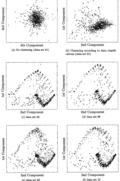
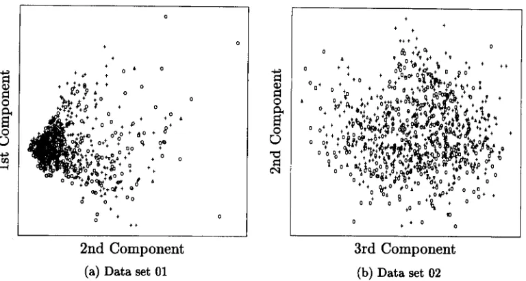
peA' plots using the moustache data sets

96

(13)

LIST OFFIGURES

4.6 PCA plots using the beard data sets 4.7 PCA plots using the eye data sets

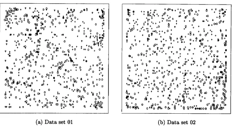
4.8 SOM plots using the moustache data sets 4.9 SOM plots using the beard data sets 4.10 SOM plots using the eye data sets

97 98 100 101 102

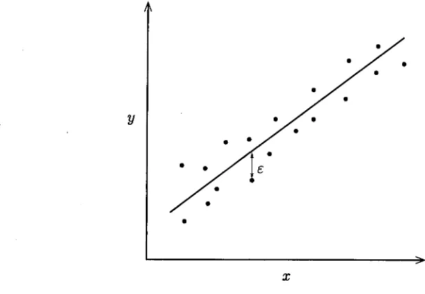
5.1 Simple linear regression . 5.2 Effect of different distance metrics

5.3 Typical error curves through the training cycle 5.4 Typical accuracy curves through the training cycle

5.5 Linear regression classification results for moustache data sets . 5.6 Euclidean distance classification results for moustache data sets

106 109 111 112 115 115 5.7 M =Si! distance classification results for moustache data sets . 116 5.8 Moustache classification - comparison of data sets (MLP network) 118 5.9 Moustache classification - comparison of data sets (RBFN) 120 5.10 Linear regression classification results for beard data sets 123 5.11 Euclidean distance classification results for beard data sets 123 5.12 M=Si! distance classification results for beard data sets. 124 5.13 Beard classification - comparison of data sets (MLP network) 125 5.14 Beard classification - comparison of data sets (RBFN) . . . . 126

6.1 Linear regression classification results for eye colour data sets 6.2 Euclidean distance classification results for eye colour data sets 6.3 Eye colour data set comparison using an MLP

6.4 Eye colour data set comparison using an RBFN .

135 138 140 146 6.5 Eye colour data set comparison between network types. 147 6.6 Single eye colour classification - comparison of data sets 154 6.7 Results from combining the outputs of five single eye colour networks

using

a

"Winner Takes All" algorithm. . . 157 6.8 Eye colour data set comparison - combining single colour networks 158 6.9 Eye colour - combining single colour networks - best results . . . . 160

(14)

LIST OF FIGURES

6.10 Eye colour - comparing the three network approaches 161

6.11 Eye colour - PDF on eye01 data 162

6.12 Eye colour - PDF on eye13 data 162

6.13 Eye colour - comparing all classification approaches . 164 6.14 Eye colour - comparing all classification approaches (no thresholds) . 164

C.1 Moustache classification - comparison of numbers of hidden neurons

(MLP network) . . . 178

C.2 Moustache classification - comparison of learning rates (MLP network) 179 C.3 Moustache classification - comparison of numbers of basis function neurons180 C.4 Moustache classification - comparison of learning rates (RBFN network) 181 C.5 Beard classification - comparison of numbers of hidden neurons (MLP

network) . . . 182 C.6 Beard classification - comparison of learning rates (MLP network) 183 C.7 Beard classification - comparison of numbers of basis function layer neurons 184 C.8 Beard classification - comparison of learning rates (RBFN network) . . . 185 C.9 Eye colour classification - comparison of numbers of hidden neurons

(MLP network) . . . .. 186 C.10 Eye colour classification - comparison of learning rates (MLP network) 187 C.ll Eye colour classification - comparison of numbers of basis function neurons188 C.12 Eye colour classification - comparison of learning rate in RBFN ... 189 C.13 Single eye colour classification - comparison of hidden layer size (MLP

network) 190

C.14 Single eye colour classification - comparison of learning rate (MLP network) 191 C.15 Combining single eye colour networks - hidden layer comparison (MLP

network) . . . 192 C.16 Combining single eye colour networks - comparison oflearning rate (MLP

network) 193

(15)

List of Tables

3.1 A typical confusion matrix. 71

77 78 85 87 87 87 88 90 97 4.1 Physically derived measures ...

4.2 Non physically derived measures 4.3 Feature points used in data location 4.4 Data sets used for moustache identification 4.5 Data sets used for beard identification 4.6 The eye colour classifications ...

4.7 Data sets used for eye colour identification . 4.8 Distribution of examples of each eye colour class 4.9 Shapes used to represent eye colours in PCA plots

5.1 Data set sizes for simple classifications . . . 105

6.1 Confusion matrices for linear regression classifier using the eye02 data set 137 6.2 Confusion matrices for Euclidean distance classifier using eye02 data . . 139 6.3 Confusion matrices for MLP network classifier using the eye02 data set. 143 6.4 Confusion matrices comparing colour data representations . . . 144 6.5 Confusion matrices for RBF network classifier using the eye02 data set. 149 6.6 Confusion matrices comparing colour data representations 150

6.7 File sizes for single eye colour data files 152

6.8 Data sets produced by combining single eye colour network responses. 156

(16)

List of Algorithms

2.1 The RCE algorithm

...

38

3.1 Percept ron learning algorithm . 57

5.1 Evaluate the repetition needed of each class to balance data sets 105

5.2 Learning scheme used for classification problems 111

6.1 Interpretation of five output networks 133

B.1 RGB to HSV conversion ... 176

(17)

Acknowledgements

The author would like to thank the followingfor their contributions to this work:

The Police Service Research and Development Group at the UK Home Office for the proposal of the work undertaken in preparing this thesis, the provision of funds for the thesis and the supply of data for carrying out the experimental work.

The Engineering and Physical Sciences Research Council for their funding of the work.

Dr. E. Hines for his supervision of the work in this thesis.

Prof. D. J. Whitehouse for his helpful comments on the structure and content of this thesis and suggestions on the direction of the work.

Dr. M. Craven, Dr. A. H. Khan, Dr. A. B. Larkin and Dr. A. C. Pardoe for friendship and support during the course of the study for this thesis.

(18)

Declaration

The work reported on in this thesis was produced by the author unless otherwise stated. All work reported here was carried out during the author's period of study while registered as a PhD student at the University of Warwick. A publication resulting from work leading to this thesis is presented in Appendix C.

(19)

Abstract

Describing a human face is a natural ability used in eveyday life. To the police, a witness description of a suspect is key evidence in the identification of the suspect. However, the process of examining "mug shots" to find a match to the description is

tedious and often unfruitful. Ifa description could be stored with each photograph and used as a searchable index, this would provide a much more effective means of using

"mug shots" for identification purposes.

A set of descriptive measures have been defined by Shepherd [73] which seek to describe faces in a manner that may be used for just this purpose. This work investigates methods of automatically determining these descriptive measures from digitised images.

Analysis is performed on the images to establish the potential for distinguishing between different categories in these descriptions. This reveals that while some of the classifications are relatively linear, others are very non-linear.

Artificial neural networks (ANNs), being often used as non-linear classifiers, are considered as a means of automatically performing the classification of the images. As a comparison, simple linear classifiers are also applied to the same problems.

The work shows that there is potential in the use of ANNs for the classification of facial features. On simple features such as the presence or absense of a beard, high accuracies between 90 and 100% were acheived. The more complex classification of eye colour yielded lower results of around 30% accuracy and further analysis is performed to show the limitations in the data sets that have produced this result.

Overall, the work shows that there is potential for ANNs techniques in this area though much further development would be needed before all of the classifications are at a standard that could be used by the police.

(20)

Chapter 1 Introduction

When a witness to a crime is interviewed by the police, one of the objectives of the interview is to identify the suspected criminal. One part of this is to make use of information held, either in paper form or on computer, regarding people with previous criminal convictions. The traditional system employed in UK Police stations for witness identification of suspects from this information could be considered rather primitive and has a low success rate[79]. Police photos of convicted criminals are kept in albums and identifying a suspect from these is simply a matter of looking through the album until a match is found. This is an ineffective system as after seeing many photographs[43], the witness is no-longer able to make correct judgement in identifying the suspect and may be misled by similar looking photographs.

What is needed is a method of reducing the number of photographs that have to be presented to the witness and thus increasing the probability that the suspect will be presented to the witness while they are still able to correctly identify them from within the set of other photographs. One method is to group the photographs by crime type. This will help in the case of crimes that have few offenders but will not aid with "common" crimes where the number of offenders in a given region is still in the 1000's.

Another approach is to group faces according to likeness and only show the witness photographs which are similar to their description of the suspect. The difficulty that arises in performing this selection is how to measure similarity i.e. which features should be used to perform the grouping. In addition, it is likely that the photographs

(21)

Introduction 2

would need to be re-grouped for each witness presentation. That is, it is likely that one "similar" grouping that was used for a given witness would not be of use for a different suspect identification. Ifthis sorting and grouping were performed manually then the work involved would be prohibitive so some form of automated system is required.

To this end, a computerised system has been developed for presenting photographs to witnesses based on their descriptions[73]. This is described in detail in Section 2.2. The system is based on a series of 50 descriptive measures that are stored in association with each facial image. These are used as an index to the library of photographs so that searches can be made for faces that match a given description. The workload here is now governed by the efforts required in the generation of the descriptive measures. This has been performed for some small databases[74] of upto 2000 faces using manual techniques [72] but such manual data entry is not suitable for adding descriptions to

hundreds of thousands of records that make up the whole of the database stored on the UK Police National Computer. Rather what is needed is an automated method of generating the descriptive measures.

Given that the images can be scanned into a digital format for computer entry, the task becomes one of interpreting these digital images to yield the descriptive measures.

This is the focus of work contained in this thesis; it may be summarised in the statement:

"Given a digitised colour image of a face, extract from that image a series of pre-defined descriptive measures."

This work is part of an ongoing project by the UK Home Office Police Science Research and Development Group which has awarded a number of research contracts to various groups as part of the overall project. The work in this thesis is specifically

(22)

1.1 What's ina Face? ₃

1.1 What's in a Face?

Given that most faces are made up from the same basic components - two eyes, two ears, one nose, one mouth and some hair on top - with the same basic arrangement, there is

a remarkable degree of variation that allows us to easily recognise familiar individuals in the midst of a crowd. Various questions arise such as "what are the variables that allow humans to perform this recognition?" "Are there measurable quantities that can be found that will allow an automatic discrimination between faces?" Psychologists have been examining these and other similar questions for many years.

There is an interesting phenomena observed in the recognition problem, in that Europeans find it easier to distinguish between other Europeans than between those of other races and vice versa[75]. This demonstrates that regular exposure to one "kind"

of face gives the human observer an ability to more easily distinguish within that group. However studies have shown[22, 23] that there is nothing inherent in the Asian face, for example, that makes Asians any more like each other than Europeans, i.e. the degree of variation in the features is the same.

One can think of many instances where some form of automated recognition system

would be beneficial such as, for example, building security systems[71]. In designing such systems, there can be great benefit in considering the psychological processes involved in human recognition. For example, the phenomena described above is one that is observed with the artificial neural networks described in the next section. That is, repeated presentation of a given subset of the available data when training the network gives a greater degree of discrimination within that subset than within larger

data set. This type of phenomena is an example of how artificial neural network systems are mimicking the behaviour of their biological counterparts. However the systems that are in existence today are still poor in their abilities when compared to human recognition.

(23)

1.2 Intelligent Computers? 4

human recognition ability is not hampered by differing facialexpressions but these can

make large differences to measurements taken from points on the face; the difference between a smile and a frown can greatly alter distances measured from the corners of the mouth. For this reason, automated recognition experiments will often be performed using "expressionless" faces. The data used in this thesis is also of this type with the faces contrained in position within the image and showing no expression. Chapter 4 details the data used in this thesis.

Other factors that produce variation in facial images are the lighting conditions, the background and the orientation of the head with respect to the camera. In many recognition experiments, these will therefore be controlled by, for example, the use of

camera lights, plain coloured backgrounds and fixed positions of the subject's head with respect to the camera. However, research has also been directed specifically at these issues, in particular Govindaraju et al.[26] have worked on identifying faces in cluttered

images while Beymer et al.[4], Lando et al.[42] and others have looked at position and rotation invariance in facial recognition.

While various researchers have looked at individual problems in facial image process-ing, each solution has been specific to a particular problem rather than being generic. There would appear to be much complex information stored in the image of a face which current processing techniques have yet to fully make use of or extract.

Chapter 2 will discuss in much greater detail the work done by other researchers in

facial image processing and show the extent of current research.

1.2 Intelligent Computers?

Artificial intelligence (AI) has developed into a fairly sizable branch of computing with the aim of using computing techniques to reproduce the intelligence observed in bio-logical systems. One area of AI involves the study of biological neural systems and

attempts to mimic their behaviour by the use of various technologies such as electron-ics, computing and optics. These systems are commonly known as Artificial Neural Networks.

(24)

pat-1.2 Intelligent Computers? 5

tern recognition problems and are an area of increasing research activity. Although sometimes shrouded in mystery, the field of ANN s is one that is now of interest to many different communities looking for an alternative method of solving complex data processing problems.

The inspiration behind ANNs is the biological neural system, that is, man is seeking after an artificial implementation of the abilities that come naturally to biological sys-tems. Man has observed the ways in which biological systems develop and learn as they

grow older and wishes now to use such properties in artificial systems. That is we wish to have electronic systems that are able to learn for themselves in the same manner that, for example, a baby learns to walk and talk. The baby has no knowledge of how the process of walking should be performed he or she simply works it out by trial and error with guidance from various teachers until it becomes a natural action. Similar situations occur in various data processing problems where there is no knowledge of a

mathematical or analytical solution to the problem. An alternative method of finding a solution is needed. The existence of "learning" systems brings about the possibility of solving these problems which defy analytical methods due to their complexity or perceived limitations in terms of, for example, the type of information required.

In addition to learning, biological systems have a natural ability to generalise, for example a child does not have to be shown every kind of dog in order to know what a dog is. Just a few examples are sufficient and from that the child generalises when

meeting other dogs. This feature of the biological neural system can be one of great benefit in some data processing problems. For example, in classification applications, it means that only a small percentage of the data population need be used in the

"training" process where the neural system learns about the task it is to perform. This brings great potential to ANNs based systems in that many problems exist where only a small percentage of the total data set is available for use in training.

(25)

1.3 The Classification Problem ₆

be seen that different neural networks do not necessarily give responses that agree

with each other. For example human descriptions of a given colour can vary wildly from one observer to another. From considering this kind of property of biological neural systems, it may be expected that similar behaviour will be experienced with the artificial counterparts. That is independently trained ANNs are likely to give different results when presented with the same input data.

For this reason a neural network system is not suitable to be applied to a problem where accurately predictable results are needed i.e. the system is required to always give the same response rather than being dependent on the particular training cycle.

This form of problem falls more into the area of algebra where a "proved" result can be given. However, there are instances where it is not possible to produce algebraic expressions or algorithms for the classification that is required. Itis in instances such as these that ANN s can be particularly powerful.

1.3 The Classification Problem

In data processing, it is common to want to classify a given piece of data as belonging to one of a number of classes. For example in a traffic census, vehicles may be classified according to type (car, lorry, bus, van etc.). In this particular case the classification is usually performed by a human observer. However, there are many cases where it would be desirable that the classification process is automated in some manner. For example, in the traffic census, suppose the human observer were replaced by a video camera. Then the input data is the image from the camera and a classification is to be

made based on that image. This could be automated given sufficient a priori knowledge about the appearance of each class of vehicle and suitable image processing algorithms.

This form of problem may be generalised by stating that in all classification prob-lems, the input data will consist of a series of vectors each describing one object to be classified. Certain rules must then be followed to determine the classification. If the input vectors are single valued, then the classification may be as simple as applying a

(26)

1.3 The Classification Problem 7

B and values above 4 to class C. However, usually the input vectors are multi-valued

and some more complex method will be used to assign the correct classes.

One method frequently used is that of Euclidean distance measures. A sample of data known as the "training data" for which the correct classification is known is

used to establish the centres of the each class, that is, taking all training data vectors belonging to a given class, the mean value is found. Then for each of the vectors that requires classification, the Euclidean distance between that vector and each of the

"cluster centres" is found according to

d= J(x-c)2. (1.1)

where x is the vector in question, c is the centre of the cluster and d is the Euclidean distance. The vector is then said to belong to the cluster whose centre it is closest to i.e. the one where the Euclidean distance is the smallest.

This is a simple method of classification which presumes that data classes are ar-ranged within the data space in groups that can be separated from each other. Unfor-tunately, this is often not the case and in these situations, more complex classification

methods are required. For example, distance measures can be modified to fit the shape of the data classes that do not follow spherical groupings around a central point; this is explained further in Section 5.1.1.

A classification problem may be thought of as a mapping function where a given in-put vector is to be mapped to a certain outin-put vector. When classification is considered

in this light artificial neural networks may be considered as a method of solving such problems that are too complex for simple Euclidean distance measures. Their learning properties enabling the networks to devise the features needed for classification. Hence neural networks, with their inputs driven by the vectors to be classified and their out-puts representing the classes, have been used in many situations where mathematical equations representing the classification have not been easy to find.

(27)

1.4 Thesis Outline 8

contain much complex information. Itis one of the principle objectives of this work to investigate, and demonstrate, the extent to which ANNs are able to extract relevant information from face images in order to perform the task of facial feature classification.

1.4 Thesis Outline

This thesis describes the work performed by the author in order to investigate the possible solution of the problem of facial feature extraction using ANNs. Chapters 2 and 3 cover the main background areas to the work and the remaining chapters present the author's contribution to this field of research. The thesis follows the structure given

below.

1.4.1 Chapter 2 - Introduction and background to facial image

pro-cessing

Chapter 2 gives an overview of the history of facial image processing. It describes the major techniques that have been used and covers some of the applications of facial

image processing including the use in police work and the history of police "mugshot" photography.

1.4.2 Chapter 3 - Introduction and background to neural networks

Chapter 3 is an introduction to artificial neural networks which covers all the techniques that are used in this work. Included in it is a description of traditional computing sys-tems and biological neural syssys-tems to explain how artificial neural networks fit into the computing framework and where the original inspiration for them came from. Mathe-matical derivations are given for the operation and learning algorithms of each of the networks along with description of typical uses of each network type.

1.4.3 Chapter 4 - Data and data pre-processing

Chapter 4 discusses the data set used for this work, how it was gathered and the

(28)

description which, although consisting of a number of numeric values, is designed to be

meaningful to a human observer. The aim of this work is to investigate the automatic extraction of these descriptive measures from the images using artificial neural network techniques. The raw data set is not suitable for presentation to artificial neural networks so a number, of different pre-processing techniques were used. Since the images were supplied in colour, it was necessary to explore different digital colour representations to find a suitable form for network training. In addition, the data was analysed using some statistical and un-supervised neural network methods to evaluate the separability of the classes involved.

1.4.4 Chapter 5 - Evaluating neural techniques using a simple

classi-fication

Chapter 5 describes the work done in applying artificial neural networks to the

clas-sification of simple facial features. The moustache and beard were taken as test cases to evaluate the potential for further development of these techniques. These are both cases of detecting the presence or absence of a feature rather than applying a classi-fication to a feature that is always present. In order to provide a reference outside of neural network methods, consideration is also given to the use of linear regression and distance measures as alternative classifiers. The details of the methods employed are presented along with the corresponding results.

1.4.5 Chapter 6 - Putting neural techniques to the test with complex

classification

Chapter 6 is concerned with neural network classification of more complex features. The facial area of the eye was chosen for this work and neural networks were applied to the

(29)

1.4.6 Chapter 7 - Conclusions and future work

Chapter 7 draws together the conclusions that may be made from this work and suggests further work that may be considered in this area.

Appendix A contains the mathematical derivation of the derivative of two activation functions that are commonly used in neural networks. See Chapter 3 for the use of these functions and their derivatives.

Appendix B contains algorithms for the conversion of RGB colour values to the CMY and HSV colour representations.

(30)

Chapter 2 Face Image Processing

Many studies have been undertaken on issues relating to the human face. It is clear from observation that faces are similar, with the basic features following a common form for most examples and yet it is possible to distinguish between many different faces and humans have seemingly amazing abilities to recognise known faces. In this

chapter, an overview is presented of the main pieces of research work that have been done on facial image processing along with a summary of the police's interests in facial images. The subject of facial recognition has been the area in which most work has

been performed and will therefore receive the most attention in this chapter.

The area of classifying facial features as performed in the experimental work of this thesis has received very little attention. That which exists is mentioned in this chapter, however it is generally based around conventional image processing techniques rather than the ANNs which are the focus of this thesis.

2.1 Conventional facial recognition techniques

The problem of facial recognition has been studied since at least the 1960's with vari-ous attempts to understand this most complicated and yet common of human abilities. Some research has looked specifically at what information is used by humans in per-forming facial recognition, and the degree of accuracy that can be achieved; while more recent studies have usually centred on computerised techniques for such recognition.

(31)

2.1 Conventional facial recognition techniques 12

2.1.1 The human ability to recognise faces

Investigations have been carried out by various researchers into the human ability to recognise faces, usually focusing on the various psychological aspects of the process. A summary of the findings of this research will now be presented.

Initial studies by Goldstein et al.[24] were performed using a group of jurors to produce descriptions of a set of 255 photographs of faces based on 34 features. Var-ious statistical analyses were performed on the descriptions to evaluate which were giving the most information and which were the most consistent between the jurors. This process reduced the set to a final list of 22 features. The recognition process was then investigated using a binary search technique where each feature of the face to be matched was taken in turn and the set of target images ranked from 0 to 1 according

to the degree of match in this feature. Only the "extreme" 1features of the target face were used and the features were matched in the order of the most extreme first. A "cutoff" criterion or threshold, p, was used such that the set was split at the point p

or 1 - P depending on the match being made and thus the target group was reduced. Investigation was made to identify the number of decisions that were required to

re-duce the set to a single photograph depending on the number in the population being searched and the value ofp. A logarithmic relationship

InN

+

In2.62

r

=

----:---lnp (2.1)

was found between the population size and the number of extreme features needed for identification, where N is the population size and r the number of features needed. Thus giving an estimate of the number of extreme features needed to uniquely identify a face from within a given population.

Harmon followed up this work[29] by looking at the amount of information needed in an image to make a face recognisable. He tried reducing the resolution of the images

by sub-sampling and then tested the resultant images on a group of subjects to evaluate the recognition rate. The results from these experiments showed a great variation in

(32)

the recognition rate from one image to another when the images were reduced to 16x16

pixels. As part of the investigation as to why this occurred, the images were re-sampled with the centres of the sub-sampled pixels moved right or down or both by half a block.

This yielded four different versions of each face and it became apparent that each of these had a different recognition rate. Using the optimum image for each of the faces doubled the recognition rate achieved to 95%. The means by which these "block portraits'v' hide data was then investigated with the conclusion that they introduce high frequency noise. This is why such images are more easily recognised if one looks at them with a squint since doing this effectively performs a low pass filter on the image.

Harmon also performed further experiments[29] on the recognition process using

both a binary style search such as Goldstein's, already described, and a rank based system which allows occasional mistakes to be made whilst still resulting in the iden-tification of the correct target. The binary sort process runs the risk of eliminating the target photograph early on in the search process by removal due to a mistake in the classification decisions. With the ranking system, at no time are any of the pho-tographs removed from the data set, rather, at each ranking operation, a weighting is

applied to each photograph based on how well the description of the feature in question is matched, thus allowing an image to still be matched with the target even if one of the feature descriptions is not correctly matched.

When the binary sort was performed by a human judge, on average 7.3 sorting oper-ations were needed to isolate a single photograph whereas with a computer performing the sorting, only six decisions were needed. In addition to replacing the binary search with a ranking process, the searching procedure was altered in these experiments in an

attempt to minimise the number of features needed to identify the correct face and to improve the accuracy of that identification.

(33)

of these "extreme" features had been entered, an automatic feature selection process was used such that the computer asked for the "most discriminating feature" at any stage of the search. This was done by examining the faces in the set being considered to evaluate which feature had the most even distribution of values. For example, if all members of the population had small eyes then a decision based upon that would not work well for discriminating. However if there was a broad range of the size of mouth then that would form a good basis for a decision. In the system implemented, the computer always asked for 10 features as equation (2.1) suggested that this would be

sufficient to identify the required target. This approach yielded accurate results with the target face ranked in first place for 70% of the trials and within the top 4% of the population for 99% of the trials.

Various psychologists have proposed theories of how the human visual[3] and recognition[9] systems work. Baron[3] examined theories of the human visual system with particular reference to the problem of human facial recognition. He devised a number of

com-puter based and neural network models to evaluate these theories. Use was made of a technique in which low resolution copies of the faces, and feature areas extracted from the faces, were stored as templates against which new images could be compared. He described neural network models for standardisation of image size and considered the transformation performed on the image by the visual cortex. Lastly he examined the effect of damage to the network systems that he proposed, showing similar behaviour

to damaged human systems. From these experiments, some insight is gained into the methods by which the human visual system is able to recognise faces. The details of exactly how the human visual system works is still well beyond our current under-standing, but what knowledge has been gained may be of use in designing automated systems for face recognition.

2.1.2 Surveys of automated face recognition

(34)

Samal and Iyengar [70] looked at five areas of the problem of facial recognition:

• Representation of faces

• Detection of faces

• Identification/Recognition of faces

• Analysis of facial expressions

• Classification based on physical features

Consideration was given to the amount of data needed to represent the image of a face such that it may still be recognisable. Itwas concluded that greyscale images at a size of 32 x 32 x 4bpp3 may be sufficient for identification purposes while it is certainly

enough for detection of a face within an image. This may be compared to the images that were used as the basis of the work in this thesis. As described in Chapter 4, they are colour images at a size of 384 x 512 x 24bpp when viewed as complete face images. The images used in this thesis, therefore, are much larger than is needed to identify the individual in the image. However, that is not the purpose of the work. This thesis is concerned with the detail of the features in the image and therefore requires images much larger than that needed for overall facial identification.

Samal and Iyengar[70] also noted many assumptions that are usually used in the facial recognition process such as the face being at a known position with no occlusion

or rotation. Frequently samples are used with no facial hair or glasses and often the population is restricted to white males within a certain age range. Bearing these limita-tions in mind, it would appear that many of the attempts at designing facial recognition systems fall far short of what may be needed in a real life working situation.

Throughout most of the various work on face image processing, faces were repre-sented in two basic forms, either using 2D intensity maps (i.e. the grey scale or colour image) or feature vectors (i.e. where individual features within the image are repre-sented collectively as a vector, e.g. a vector denoting the outline of the an eye). The intensity map is the approach used in the template matching described in Section 2.1.3.

(35)

Its main drawback is that it generally requires comparatively large storage for each face, although if the minimum size of 32x 32x 4 already discussed is used, then the storage requirement is 512 bytes per face. In comparison, the images used for the work in this thesis are large at 589,824 bytes in size. However, this full size image is only being used as the source from which descriptive measures are to be calculated and will not be stored after that. See Chapter 4 for details on the data used in this thesis and the descriptive measures evaluated.

Feature vectors are derived from two basic sources - either the intensity map or a face profile. The first type are typically measures such as size of eyes, distance between eyes, size of mouth etc. Features from profile images are obtained from a set of points on the profile from which various distances and angles are measured (see Section 2.1.5 for some work in this area).

The detection and location of a face within an image, possibly containing a cluttered background, is an area in which much less work has been done as most recognition systems assume that the face is in the image within certain bounds. A system has been developed by Govindara et al. for locating faces within newspaper photographs[26], making use of the caption information to determine the number of faces that are present. This system matches against a simple model of a face outline consisting of two vertical straight lines and two arcs. The faces must be upright and unoccluded within the image for this approach to work. Others such as Craw et al.[13] have matched against more complex templates, using a multi-resolution method, starting with coarse images and moving to finer detail to give the accurate location.

Alternatively, the face image is located by finding some component part of the face and then deriving the overall face location from this information. This moves into the area of feature location such as is discussed on page 20 using deformable templates and other techniques such as the Hough transform.

(36)

processing either full face images or face profiles. The matching process is performed by a number of different techniques, often based on Euclidean distance, clustering, set partitioning or correlation methods. The precise technique used will depend on the features involved in the matching system; for example, a grey scale matching process may well be. suited to correlation techniques whereas those representations with small vectors may be better served by a Euclidean distance measure.

2.1.3 Template and feature-based matching

systems

As mentioned in Section 2.1.2, two basic methods are generally used for automated

face recognition. That is, using either sections of face image, possibly the whole face, or measures taken from the individual features that make up the face. The latter may be referred to as feature-based systems or feature vector systems. The term template

has been used with different meaning by different authors. In some cases it refers to areas of the image that are used in the matching process, whereas in others it refers to

a model that is to be fitted to a given feature within the face images.

Brunelli and Poggio[7] compared the merits of using template matching and feature-based matching in facial recognition. In this case, they use the term template matching to refer to the use of image segments for the matching process. The feature based system[8] that they used searches for the locations of various key features on the face such as the eyes and mouth and uses these as an index into the database of faces to be matched against. The template matching system that they implemented was based on comparisons of grey level images of faces. The images are first normalised by making use of the positions of the eyes; the images are rotated, re-scaled and shifted such that the eye centres appear at fixed positions in all the images. This is done to eliminate variation in a face image due to position of the face within the image and distance of the face from the camera.

(37)

sys-2.1 Conventional facial recognition techniques 18

tem was implemented, starting with a low resolution version of the image to identify the 'correctness' of search.

Four different schemes were then adopted to overcome variations due to illumina-tion, including scaling of the image intensity" and use of the intensity gradient", The comparisons were then performed using a cross-correlation function, in which the un-known image was compared with each stored image in the database. The work showed that template matching yielded a higher recognition accuracy (around 97%, compared with 90% for the feature vector) and used a simpler method. However the feature matching approach gave the possibility for higher speed of operation and a reduced memory requirement since the data for each face was held within 35 bytes compared with typically several hundred bytes needed for the templates.

In Brunelli and Poggio's work[7],various techniques were used for feature extraction including the following. Integral projection was used in order to locate both the nose and the mouth. In this process the pixel values are summed over an area in either the vertical or horizontal direction and the shape of the resulting histogram is used to detect the presence of certain features. The vertical integral projection is defined as

Y2

V(x)

=

2:

I(x, y) ,

Y=Yl

(2.2)

whereI(x, y) is the image andYl andY2 are the vertical limits over which the integration is to be performed. For example in the detection of the nose, the absence / presence of peaks in the vertical projection is used to delimit the nose horizontally.

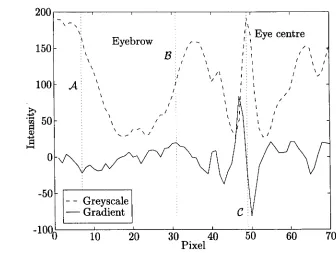
Another technique used by Brunelli and Poggio for feature location employs the gradient information contained within the grey scale image. For example, using the vertical gradient map, the eyebrows are found by looking for two peaks in the gradient information in opposite directions; the search area being limited to just above the eye position. An example of this using data taken from the data sets used in this thesis is shown in Figure 2.1. This shows the gradient values of a set of pixels on a straight line running vertically through the centre of one of the eyes. Also shown is the grey-scale

4generating pixel values as the ratio of the local value over the average brightness in a suitable neighborhood

(38)

2.1 Conventional facial recognition techniques 19

200

)

'-, !I

\: _{I I}Eye centre

\ _Eyebrow I: I

150

:\ I: I /

,

_B I I

,:

I

I I

,

I I I _I I

I I

I I _I I _, _I

,

:I I II I: I I .,.

100

_A I _I / I

I' _I I

I. I 1

/

>. I

...,

,

I

....

₅₀

I I

~ I

/ ...\ .I

I

,

Cl) _\.1 ~ I-t

0 -50

- - Greyscale - Gradient

-1000

10

20

30

40

50

60

70

[image:38.494.78.414.72.328.2]

Pixel

Figure 2.1 Gradient intensity used to locate eyebrows

values from which this gradient information was derived. The right most vertical dotted line, C, denotes the position of the centre of the eye with the peak in the grey-scale corresponding to a white reflection in the pupil of the eye. The other two vertical dotted lines,A and B,show the two peaks in the gradient, one positive and one negative that would identify the position of the eyebrow in this instance. The left hand side of the plot corresponds to the top of the image. In the system implemented by Brunelli and Poggio, these 'pairs of peaks' are compared for the two eyes and the most similar in terms of distance from the eye centre and thickness are chosen as the correct pair.

(39)

2.1 Conventional facial recognition techniques 20

of five templates of differing sizes taken from images of one of the authors' eyes. The face images were then scaled by using the size ratio of the template which returned the greatest correlation with the face in question. That is, for example, if the template of an eye scaled to 0.85 times the original size gave the greatest correlation, then the face image was increased in size by a ratio of 0.85:l. Following this, the positions of the eyes were refined using left and right eye templates and rotation is compensated for by requiring that the eyes be on a horizontal line. The final step was to re-scale the image to give a fixed inter-ocular distance. This approach has proved to give a reliable method of normalisation.

The process of normalisation highlights an important area in the processing of facial images - that is the scale of the images needs to be consistent for the subsequent work to have any meaning. In a case like this where faces are to be matched, there is an obvious need for the techniques being used to be independent of the scale of the images. The same is true for the process of extracting a description of a face from an image.Ifthe description is to include measures based on the physical aspects of the face, then it is important that the size of the images is consistent otherwise the descriptions based on these measures will have no meaning due to variation in the image scale. However, the feature classification performed in this thesis was done without any scaling of the images since the photographs were taken under controlled conditions resulting in identical scaling in the images. See Chapter 4 for details on the data used in this thesis.

Huang and Chen[36] used two methods for the location of facial features. The first approach, the deformable template, makes use of a priori knowledge about the shape of a feature to guide the contour deformation process. The template consists of an outline shape for the feature in question which may be deformed by altering a number of parameters. The deformation is an energy minimisation process which works on an energy function linked to suitable features such as peaks and valleys in the image intensity. The deformable template approach is advantageous compared with traditional edge detection routines in that it takes a more global view of the problem.

(40)

of the deformable template identifying the wrong region of the image as compared with edge detection routines which do not inherently employ this "knowledge" of the object they are locating.

The second technique used by Huang and Chen was the active contour model or snake which is an energy-minimising spline guided by external constraint forces and influenced by "image forces" such as lines and edges. These do not require their targets to be constrained in their shape as much as the deformable templates do, and are thus suited to extracting features such as eyebrows or face outline that are not so consistent in shape from one face to another.

In their work, Huang and Chen precede both the deformable template routine and the active contour by a rough estimation of the desired position of the features. This is done using what Huang and Chen call their "Rough Contour Estimation Routine" (RCER) which makes use of geometric presumptions to find a starting point for the estimation. For example in the location of the left eyebrow, the RCER presumes that its position is about 1/4 facial width.

While their work[36] is aimed at the recognition process, only the feature extrac-tion is menextrac-tioned in their paper. No detail is given as to how the system could be implemented as a working recognition system. It is the view of this author that the recognition process would involvethe matching of the extracted features; although with the active contours in their current form there would be considerable data to be stored and compared.

(41)

Two different templates were used in the mouth position location, one for an open mouth and one for a closed mouth. In both the eye and mouth location algorithms, the search was implemented over a number of iterations, where the search coefficients linking the template to the valleys and peaks were varied as the search progressed. If the search starts above the eye, then problems are encountered with the peaks which are often found around the eyebrows. Their work was extended to perform tracking of an eye through a series of frames which gives good results provided that the eye does not move significantly between frames. This was probably due to the fact that they were using the template position from framenas the starting point for framen

+

1 and as has been mentioned above, the template only performs well when its initial position is in the 'region' of the feature that is to be located.

In this context, it would appear that deformable templates could be defined for other features within the face outline such as the nose. What is less certain is to what extent the principle could be generalised for "external" features such as the ears or hairline. Another aspect of the work by Yuille et al. that needs consideration is concerned with the need for some mechanism to permit interaction between the templates for the various features such that their geometrical relationship to each other is considered when evaluating a possible positioning of the template. To date, this author has not found any work in these areas.

(42)

2.1 Conventional facial recognition techniques 23

of the real face. In the comparison of recognition rates, the use of the 15 real views gave a recognition rate of 98% whereas the virtual views achieved only 85%. This is to be compared to the case of using one view and its mirror reflection where a rate of 70% was achieved. The high recognition rate when only camera based images are used might be expected since this is simply a case of finding an exact match within the data base. A recognition rate of 85% using the virtual faces shows that the technique used for producing these images yields a good representation of the face when rotated in the manner described and shows significant improvement over the use of a single view.

2.1.4 The Karhunen-Loeve transform and "Eigenfaces"

Digitised images of faces often have large storage requirements, for example a 256 x 256 pixel image with each pixel representing one of a possible 256 grey levels will need 64Kb of storage if no compression technique is used on the image. While this is not a vast amount of space if only a few images are to be stored, the requirements can become very large if the database consists of thousands of face images. Standard image compression techniques such as those used in the GIF, TIFF or JPEG image formats may be used to reduce the image size but better compression may be achieved if a technique is devised that usesa priori knowledge of the problem.

The Karhunen-Loeve transform, otherwise known as principal components analy-sis (PCA)[38] (see Section 4.4.1 for work using PCA in this theanaly-sis), has been used by Sirovich and Kirby[78, 39] as a data compression method for the storage of face im-ages. The principal components of an ensemble of faces were calculated and used as the basis of an optimal co-ordinate system on which faces from both within and outside the original ensemble could be mapped. Investigation revealed that 50 principal com-ponents produced a good likeness of faces that were not part of the set used to form the principal components, giving around a 100:1 reduction in the data stored from the original images.

(43)

process, using the Karhunen-Loeve transform, is an alternative to the standard template matching procedures that are used to locate a given object within an image. It consists of calculating the "distance-from-face-space" of each pixel in the image to determine the "faceness" of any given pixel and thereby locate the face. This scheme allows for

a greater distortion in the object that is to be detected and has been shown to give superior performance to matched filtering[41]. This system is intended as a possible compression method for use in video telephony or some similar application where high levels of compression are needed. It's effectiveness is demonstrated in [55] by comparison with a JPEG image at the lowest quality". This yields a 540 byte image which is barely recognisable as a face, whereas the 85 byte Karhunen-Loeve representation is a close

match to the originaL

Turk and Pentland[81] used the same method of principal components analysis and gave it the name "eigenfaces". The method of eigenface encoding may be thought of as a form of feature based coding of the facial image. However, in this approach, the features are not individual sections of the face such as eyes or nose, but rather

are the principal components of a collection of images; thus the features have little meaning to the human observer. In their work, Turk and Pentland looked at the application of eigenfaces for recognition, using the eigenface method to reduce the storage requirements and computation requirements in comparing a new face to those stored in the database of known faces. In addition to reducing the data storage and computation requirements of the matching process, the use of eigenfaces transforms the images into an optimal co-ordinate system for the representation of faces and therefore

improves the matching accuracy and aids the detection of images that do not contain faces.

Moghaddam and Pentland[54] have further investigated the use of the eigenface rep-resentation for facial recognition, using the eigenfaces to detect rotation in the image about the y-axis, thus producing a rotation invariant recognition system. Their work

is a good demonstration of a practical system that yields high accuracies of 95%

recog-6A JPEG imageis created using a compression technique that involves loss of the original data.

(44)

2.1 Conventional facial recognition techniques

25

nition rate using a database of approximately 7500 photographs taken of around 3000 people with a mix of age and ethnic group. Further, using "eigenfeatures" they have produced a method of facial feature location yielding a 94% detection rate compared to a more traditional sum-of-square-differencesmatching method which gave only 75%. Then, using these eigenfeatures to code the face images, they established a method of facial recognition that showed a greater invariance to distortions in the image than the whole face, eigenfacemethod. The combined use of the whole face and the eigenfeatures resulted in a 98% accuracy in recognition.

Jiang[37] has combined eigenfaces with neural networks in his attempt at a face recognition system. The eigenface representation of faces are used as the input to an artificial neural system that has been trained to identify the face. The face images are represented by the first 100 eigenvalues, dramatically reducing the data size from the original 46 x 46 pixel image. While the reported recognition rates are high at more than 95%, the database size used in this particular work is small, i.e. only six different people, and therefore the technique needs to be tested in terms of scalability up to the kind of database sizes that may be seen in "real world" applications. See Section 2.3 for further information on face image processing using artificial neural networks.

2.1.5 Use of profile face images

Thus far, with the exception of the systems that have attempted to be rotation in-variant, all the face recognition systems presented have used full face images. Other possibilities are available and some researchers have investigated them.

(45)

[image:45.494.56.309.73.310.2]

1

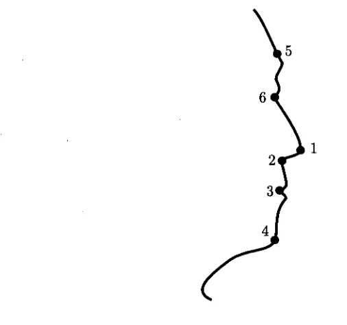
Figure 2.2 Profile points used by Wu and Huang

the straight line between forehead and the nose.

From these six "points of interest" , five features were calculated for each of the five curve segments connecting the points. These were:

• Distance between points (as a straight line.)

• Angle between curve segment and the neighbouring curve segment.

• Length of curve segment.

• Summation of curvature values at each point.

• Symmetrical measure of the curve segment.