Almost Periodic Oscillation in a Watt-type
Predator-prey Model with Diffusion and Time
Delays
Liyan Pang and Tianwei Zhang
Abstract—In this paper, we consider a Watt-type predator-prey model with diffusion and time delays. Firstly, by means of Mawhin’s continuation theorem of coincidence degree theory, some new sufficient conditions are obtained for the existence of at least one positive almost periodic solution for the above model. Secondly, by using the comparison theorem, we give a permanence result for the model. Thirdly, by constructing a suitable Lyapunov functional, the global asymptotical stability of the model is also investigated. To the best of the author’s knowledge, so far, the results in this paper are completely new. Finally, an example and numerical simulations are employed to illustrate the main result of this paper.
Index Terms—Almost periodicity, Coincidence degree, Predator-prey, Watt-type, Diffusion.
I. INTRODUCTION
I
T is well-known that the theoretical study of predator-prey systems in mathematical ecology has a long history starting with the pioneering work of Lotka and Volterra[1,2]. The principles of Lotka-Volterra model, conservation of mass and decomposition of the rates of change in birth and death processes, have remained valid until today and many theoretical ecologists adhere to these principles. This general approach has been applied to many biological systems in particular with functional response. In population dynamics, a functional response of the predator to the prey density refers to the change in the density of prey attached per unit time per predator as the prey density changes. During the last ten years, there has been extensively investigation on the dynamics of predator-prey models with the different func-tional responses in the literature, (see [3-13] and references therein).
In the last few years, mathematicians and ecologists have been actively investigating the dispersal of populations, a ubiquitous phenomenon in population dynamics. Levin (1976) showed that both spatial dispersal of populations and population dynamics are much affected by spatial hetero-geneity. In real life, dispersal often occurs among patches in ecological environments; because of the ecological effects of human activities and industries, such as the location of manufacturing industries and the pollution of the atmosphere, soil and rivers, reproduction- and population-based territories and other habitats have been broken into patches. Thus, realistic models should include dispersal processes that take
Manuscript received June 26, 2014; revised August 20, 2014.
Liyan Pang is with the School of Mathematics and Computer Science, Ningxia Normal University, Guyuan, Ningxia 756000, China. ([email protected]).
Tianwei Zhang is with the City College, Kunming University of Science and Technology, Kunming 650051, China. ([email protected]).
Correspondence author: Tianwei Zhang. ([email protected]).
into consideration the effects of spatial heterogeneity. A large number of predator-prey models for diffusion have been studied by many researchers (see [14-22] and references therein).
In [22], Lin et al. considered the following T-periodic Watt-type predator-prey system [22-26] with diffusion:
˙
x1(t) = x1(t) [r1(t)−b1(t)x1(t)]
−a1(t)y(t) [
1−exp (
−c(t)x1(t)
ym(t)
)]
+D1(t) [x2(t)−x1(t)],
˙
x2(t) = x2(t) [r2(t)−b2(t)x2(t)] +D2(t) [x1(t)−x2(t)],
˙
y(t) = y(t) [r3(t)−b3(t)y(t)] +a2(t)y(t)
[ 1−exp
(
−c(t)x1(t)
ym(t)
)] ,
(1.1)
where x1(t) and y(t) are the densities of prey species
and predator species in patch I at time t, and x2(t) is
the density of prey species in patch II, prey species x1(t)
andx(t)can diffuse between two patch while the predator
species y(t) is confined to patch I. Under the assumption of periodicity of the coefficients of system (1.1), Lin et al. studied the existence of at least one positive periodic solution of system (1.1) by means of Mawhin’s continuation theorem of coincidence degree theory.
Since biological and environmental parameters are natural-ly subject to fluctuation in time, the effects of a periodicalnatural-ly varying environment are considered as important selective forces on systems in a fluctuating environment. Therefore, models should take into account the seasonality of the period-ically changing environment. However, in applications, if the various constituent components of the temporally nonunifor-m environnonunifor-ment is with incononunifor-mnonunifor-mensurable (nonintegral nonunifor- multi-ples, see Example 1) periods, then one has to consider the environment to be almost periodic since there is no a priori reason to expect the existence of periodic solutions. Hence, if we consider the effects of the environmental factors, almost periodicity is sometimes more realistic and more general than periodicity. In recent years, the almost periodic solution of the continuous models in biological populations has been studied by many authors (see [27-34] and the references cited therein).
Example 1. Consider the following simple predator-prey model:
˙
x1(t) = x1(t) [
1−[2 + sin(√2t)]x1(t) ]
,
˙
x2(t) = x2(t) [
1−[2 + sin(√3t)]x2(t) ]
,
˙
y(t) = y(t)[1−[2 + sin(√5t)]y(t)] +y(t)
[ 1−exp
(
−x1(t)
y(t) )]
.
(1.2)
IAENG International Journal of Applied Mathematics, 45:2, IJAM_45_2_03
In system (1.2), corresponding to system (1.1), b1(t) =
2 + sin(√2t)is√2π-periodic function,b2(t) = 2 + sin(
√ 3t)
is 2
√
3
3 π-periodic function andb3(t) = 2+sin(
√ 5t)is2
√
5 5 π
-periodic function, which imply that system (1.2) is with incommensurable periods. Then there is no a priori reason to expect the existence of positive periodic solutions of system (1.2). Thus, it is significant to study the existence of positive almost periodic solutions of system (1.2).
In addition, to reflect that the dynamical behavior of the models depends on the past history of the system, it is often necessary to incorporate time delays into the models. Therefore, a more realistic model should be described by delayed differential equations [8,14-18]. Motivated by the above reasons, the aim of this paper is to consider the following almost periodic Watt-type predator-prey model with diffusion and time delays:
˙
x1(t) = x1(t) [r1(t)−b1(t)x1(t)−d1(t)x2(δ(t))]
−a1(t)y(τ(t)) [
1−exp (
−c(t)x1(t)
ym(τ(t))
)]
+D1(t) [x2(t)−x1(t)],
˙
x2(t) = x2(t) [r2(t)−b2(t)x2(t)−d2(t)x1(ζ(t))] −a2(t)y(σ(t))
[ 1−exp
(
−c(t)x2(t)
ym(σ(t))
)]
+D2(t) [x1(t)−x2(t)],
˙
y(t) = y(t) [r3(t)−b3(t)y(t)] +a3(t)y(t)
[ 1−exp
(
−c(t)x1(t)
ym(t)
)]
+a4(t)y(t) [
1−exp (
−c(t)x2(t)
ym(t) )]
,
(1.3)
whereri(1,2,3)are intrinsic growth rate,bi(1,2,3)are the
rate of intra-specific competition,di(i= 1,2)are parameters
representing competitive effects between two prey, ai(i =
1,2) are coefficients of decrease of prey species due to predation,ai(i= 3,4)are equal to the transformation rate of
predator,Di(i= 1,2)are the dispersal rate of prey species,
δ, ζ, τ and σare time delays satisfying δ(t)≤t,ζ(t)≤t,
τ(t)≤t, σ(t)≤t,limt→∞δ(t) =∞, limt→∞ζ(t) =∞,
limt→∞τ(t) =∞and limt→∞σ(t) =∞,m is a
nonneg-ative constant. Throughout this paper, we assume that all coefficients in system (1.3) are nonnegative almost periodic functions.
It is well known that Mawhin’s continuation theorem of coincidence degree theory is an important method to investigate the existence of positive periodic solutions of some kinds of non-linear ecosystems (see [35-43]). However, it is difficult to be used to investigate the existence of positive almost periodic solutions of non-linear ecosystems. Therefore, to the best of the author’s knowledge, so far, there are scarcely any papers concerning with the existence of positive almost periodic solutions of system (1.3) by using Mawhin’s continuation theorem. Therefore, the main purpose of this paper is to establish some new sufficient conditions on the existence of positive almost periodic solutions of system (1.3) by using Mawhin’s continuous theorem of coincidence degree theory.
LetR,ZandN+ denote the sets of real numbers, integers
and positive integers, respectively, C(X,Y) and C1(X,Y)
be the space of continuous functions and continuously differential functions which map X into Y, respectively. Especially, C(X) :=C(X,X),C1(X) :=C1(X,X). Related to a continuous bounded function f, we use the following
notations:
f−= inf
s∈Rf(s), f
+= sup
s∈R
f(s), |f|∞= sup
s∈R
|f(s)|.
The organization of this Letter is as follows. In Section2, we make some preparations. In Section3, by using Mawhin’s continuation theorem of coincidence degree theory, we es-tablish sufficient conditions for the existence of at least one positive almost periodic solution to system(1.3). In Sections 4-5, the uniform persistence and global asymptotical stability of system (1.3) are considered. Finally, an example and numerical simulations are also given to illustrate the main result in this paper.
II. PRELIMINARIES
Definition 1. ([44,45]) x ∈ C(R,Rn) is called almost
periodic, if for any ϵ > 0, it is possible to find a real number l = l(ϵ) > 0, for any interval with length l(ϵ), there exists a number τ = τ(ϵ) in this interval such that
∥x(t+τ)−x(t)∥ < ϵ, ∀t ∈ R, where ∥ · ∥ is arbitrary norm ofRn.τ is called to theϵ-almost period ofx,T(x, ϵ)
denotes the set of ϵ-almost periods for xand l(ϵ) is called to the length of the inclusion interval for T(x, ϵ). The collection of those functions is denoted byAP(R,Rn). Let
AP(R) :=AP(R,R).
Lemma 1. ([44,45])Ifx∈AP(R), thenxis bounded and uniformly continuous onR.
Lemma 2. [29]Assume thatx∈AP(R)∩C1(R)withx˙ ∈ C(R), for ∀ϵ >0, we have the following conclusions:
(I) there is a point ξϵ ∈ [0,+∞) such that x(ξϵ) ∈
[x∗−ϵ, x∗]and x˙(ξϵ) = 0;
(II) there is a point ηϵ ∈ [0,+∞) such that x(ηϵ) ∈
[x∗, x∗+ϵ]and x˙(ηϵ) = 0.
The method to be used in this paper involves the appli-cations of the continuation theorem of coincidence degree. This requires us to introduce a few concepts and results from Gaines and Mawhin [46].
LetXandYbe real Banach spaces,L: DomL⊆X→Y
be a linear mapping andN :X→Ybe a continuous map-ping. The mappingLis called a Fredholm mapping of index zero ifImL is closed in Yand dimKerL= codimImL <
+∞. If L is a Fredholm mapping of index zero and there exist continuous projectorsP :X→XandQ:Y→Ysuch that ImP = KerL,KerQ= ImL= Im(I−Q). It follows that L|DomL∩KerP : (I−P)X →ImL is invertible and its
inverse is denoted byKP. IfΩis an open bounded subset of X, the mappingN will be calledL-compact onΩ¯ ifQN( ¯Ω)
is bounded and KP(I−Q)N : ¯Ω→ X is compact. Since
ImQ is isomorphic to KerL, there exists an isomorphism
J : ImQ→KerL.
Lemma 3. ([46])LetΩ⊆Xbe an open bounded set, Lbe a Fredholm mapping of index zero andN be L-compact on
¯
Ω. If all the following conditions hold:
(a) Lx̸=λN x, ∀x∈∂Ω∩DomL, λ∈(0,1); (b) QN x̸= 0, ∀x∈∂Ω∩KerL;
(c) deg{J QN,Ω∩KerL,0} ̸= 0,whereJ : ImQ→KerL
is an isomorphism.
ThenLx=N xhas a solution onΩ¯∩DomL.
IAENG International Journal of Applied Mathematics, 45:2, IJAM_45_2_03
Under the invariant transformation (x1, x2, x3)T =
(eu, ev, ew)T, system (1.3) reduces to
˙
u(t) = r1(t)−b1(t)eu(t)−d1(t)ev(δ(t))
−a1(t)ew(τ(t))−u(t) [
1
−exp(−c(t)eu(t)−mw(τ(t))) ]
+D1(t)[ev(t)−u(t)−1]:=F1(t),
˙
v(t) = r2(t)−b2(t)ev(t)−d2(t)eu(ζ(t))
−a2(t)ew(σ(t))−v(t) [
1
−exp(−c(t)ev(t)−mw(σ(t))) ]
+D2(t)[eu(t)−v(t)−1]:=F2(t),
˙
w(t) = r3(t)−b3(t)ew(t)
+a3(t)[1−exp(−c(t)eu(t)−mw(t))]
+a4(t)[1−exp(−c(t)ev(t)−mw(t))]
:=F3(t).
(2.1)
Forf ∈AP(R), we denote by
¯
f =m(f) = lim
T→∞
1
T ∫ T
0
f(s) ds,
Λ(f) = {
ϖ∈R: lim
T→∞
1
T ∫ T
0
f(s)e−iϖsds̸= 0 }
,
mod(f) = {∑m
j=1
njϖj:nj∈Z, m∈N, ϖj∈Λ(f)
}
the mean value, the set of Fourier exponents and the module of f, respectively.
SetX=Y=V1 ⊕
V2, where
V1=
{
z= (u, v, w)T ∈AP(R,R3) : mod(u)⊆mod(Lu),mod(v)⊆mod(Lv),
mod(w)⊆mod(Lw),∀ϖ∈Λ(u)∪Λ(v),|ϖ| ≥θ0
} ,
V2=
{
z= (u, v, w)T ≡(k1, k2, k3)T, k1, k2, k3∈R},
where
Lu= r1(t)−b1(t)eφ1(0)−d1(t)eφ2(δ(0))
−a1(t)eφ3(τ(0))−φ1(0) [
1
−exp(−c(t)eφ1(0)−mφ3(τ(0))) ]
+D1(t)[eφ2(0)−φ1(0)−1], Lv= r2(t)−b2(t)eφ2(0)−d2(t)eφ1(ζ(0))
−a2(t)eφ3(σ(0))−φ2(0) [
1
−exp(−c(t)eφ2(0)−mφ3(σ(0))) ]
+D2(t)[eφ1(0)−φ2(0)−1], Lw= r3(t)−b3(t)eφ3(0)
+a3(t)[1−exp(−c(t)eφ1(0)−mφ3(0))]
+a4(t)[1−exp(−c(t)eφ2(0)−mw(t))], φ = (φ1, φ2, φ3)T ∈ C([−τ,0],R3), τ = maxi=1,2,3;i̸=j{τ+, δ+, σ+, ζ+}, θ0 is a given positive
constant. Define the norm
∥z∥X= max {
sup
s∈R
|u(s)|,sup
s∈R
|v(s)|,sup
s∈R
|w(s)| }
,
wherez= (u, v, w)T ∈X=Y.
Similar to the proof as that in articles [29], it follows that
Lemma 4. XandYare Banach spaces endowed with∥·∥X.
Lemma 5. LetL:X→Y,Lz=L(u, v, w)T = ( ˙u,v,˙ w˙)T, thenLis a Fredholm mapping of index zero.
Lemma 6. DefineN :X→Y,P:X→XandQ:Y→Y
by
N z=N uv
w =
F1F2((tt))
F3(t) ,
P z=P uv
w =
u¯¯v
¯
w =Qz.
ThenN isL-compact onΩ(Ω¯ is an open and bounded subset ofX).
III. MAIN RESULTS
Now we are in the position to present and prove our result on the existence of at least one positive almost periodic solution for system (1.3).
(H1) b−i >0,i= 1,2,3.
And define
ρ+1 =ρ+2 = max {
ln [
r+1 b−1 ]
,ln [
r2+ b−2
]}
, ρ−3 = ln [
r−3 b+3 ]
,
ρ+3 = ln [
r+3 +a+3 +a+4 b−3
] ,
ϱ= max{(1−m)ρ−3,(1−m)ρ+3}, µ1(s) =r1(s)−d1(s)eρ
+ 2 −a
1(s)c(s)eϱ, µ2(s) =r2(s)−d2(s)eρ+1 −a2(s)c(s)eϱ, ∀s∈R.
Theorem 1. Assume that (H1)and the following condition hold:
(H2) µ−j >0,j= 1,2,
then system(1.3)admits at least one positive almost periodic solution.
Proof: It is easy to see that if system (2.1) has one almost periodic solution (¯u,v,¯ w¯)T, then (eu¯, e¯v, ew¯)T is a
positive almost periodic solution of system (1.3). Therefore, to completes the proof it suffices to show that system (2.1) has one almost periodic solution.
In order to use Lemma 3, we set the Banach spacesXand
Y as those in Lemma 4 and L, N, P, Q the same as those defined in Lemmas 5 and 6, respectively. It remains to search for an appropriate open and bounded subsetΩ⊆X.
IAENG International Journal of Applied Mathematics, 45:2, IJAM_45_2_03
Corresponding to the operator equation Lz = λz, λ ∈
(0,1), we have
˙
u(t) = λ {
r1(t)−b1(t)eu(t)−d1(t)ev(δ(t))
−a1(t)ew(τ(t))−u(t) [
1
−exp(−c(t)eu(t)−mw(τ(t))) ]
+D1(t) [
ev(t)−u(t)−1] },
˙
v(t) = λ {
r2(t)−b2(t)ev(t)−d2(t)eu(ζ(t))
−a2(t)ew(σ(t))−v(t) [
1
−exp(−c(t)ev(t)−mw(σ(t))) ]
+D2(t)[eu(t)−v(t)−1] },
˙
w(t) =λ {
r3(t)−b3(t)ew(t)
+a3(t)[1−exp(−c(t)eu(t)−mw(t))]
+a4(t)[1−exp(−c(t)ev(t)−mw(t))] }.
(3.1)
Suppose that z = (u, v, w)T ∈ DomL ⊆ X is a solution
of system (3.1) for some λ∈(0,1), whereDomL={z= (u, v, w)T ∈X:u, v, w∈C1(R),u,˙ v,˙ w˙ ∈C(R)}.
By Lemma 2, for ∀ϵ∈(0,1), there are four points ξi =
ξi(ϵ),ηi=ηi(ϵ) (i= 1,2,3) such that
{ ˙
u(ξ1) = 0,
u(ξ1)∈[u∗−ϵ, u∗], {
˙
v(ξ2) = 0,
v(ξ2)∈[v∗−ϵ, v∗],
(3.2)
{ ˙
w(ξ3) = 0,
w(ξ3)∈[w∗−ϵ, w∗], {
˙
u(η1) = 0,
u(η1)∈[u∗, u∗+ϵ],
(3.3)
{ ˙
v(η2) = 0,
v(η2)∈[v∗, v∗+ϵ], {
˙
w(η3) = 0,
w(η3)∈[w∗, w∗+ϵ], (3.4)
where u∗ = sups∈Ru(s), v∗ = sups∈Rv(s), w∗ =
sups∈Rw(s), u∗ = infs∈Ru(s), v∗ = infs∈Rv(s), w∗ =
infs∈Rw(s).
From system (3.1), it follows from (3.2)-(3.4) that
0 = r1(ξ1)−b1(ξ1)eu(ξ1)−d1(ξ1)ev(δ(ξ1))
−a1(ξ1)ew(τ(ξ1))−u(ξ1) [
1−exp(−c(ξ1)eu(ξ1)−mw(τ(ξ1)) )]
+D1(ξ1)[ev(ξ1)−u(ξ1)−1],
0 = r2(ξ2)−b2(ξ2)ev(ξ2)−d2(ξ2)eu(ζ(ξ2))
−a2(ξ2)ew(σ(ξ2))−v(ξ2) [
1−exp(−c(ξ2)ev(ξ2)−mw(σ(ξ2)))]
+D2(ξ2)[eu(ξ2)−v(ξ2)−1],
0 = r3(ξ3)−b3(ξ3)ew(ξ3)
+a3(ξ3)[1−exp(−c(ξ3)eu(ξ3)−mw(ξ3))]
+a4(ξ3)[1−exp(−c(ξ3)ev(ξ3)−mw(ξ3))]
(3.5) and
0 = r1(η1)−b1(η1)eu(η1)−d1(η1)ev(δ(η1))
−a1(η1)ew(τ(η1))−u(η1) [
1−exp(−c(η1)eu(η1)−mw(τ(η1)))]
+D1(η1) [
ev(η1)−u(η1)−1],
0 = r2(η2)−b2(η2)ev(η2)−d2(η2)eu(ζ(η2))
−a2(η2)ew(σ(η2))−v(η2) [
1−exp(−c(η2)ev(η2)−mw(σ(η2)) )]
+D2(η2)[eu(η2)−v(η2)−1],
0 = r3(η3)−b3(η3)ew(η3)
+a3(η3) [
1−exp(−c(η3)eu(η3)−mw(η3) )]
+a4(η3)[1−exp(−c(η3)ev(η3)−mw(η3))].
(3.6)
By the third equation of system (3.5), it follows that
b3(ξ3)ew(ξ3)
=r3(ξ3) +a3(ξ3) [
1−exp (
−c(ξ3)eu(ξ3)−mw(ξ3) )]
+a4(ξ3) [
1−exp (
−c(ξ3)ev(ξ3)−mw(ξ3) )]
≤r3++a+3 +a+4,
which yields
w(ξ3)≤ln [
r3++a+3 +a+4 b−3
] :=ρ+3.
From (3.3), we have
w∗≤w(ξ3) +ϵ≤ρ+3 +ϵ.
Lettingϵ→0 in the above inequality leads to
w∗≤ρ+3. (3.7) From the third equation of system (3.6), it follows that
b+3ew(η3)
≥b3(η3)ew(η3)
=r3(η3) +a3(η3) [
1−exp (
−c(η3)eu(η3)−mw(η3) )]
+a4(η3) [
1−exp (
−c(η3)ev(η3)−mw(η3) )]
≥r3−,
which yields
w(η3)≥ln [
r3− b+3 ]
.
From (3.4), we have
w∗≥w(η3)−ϵ≥ln [
r3− b+3 ]
−ϵ.
Lettingϵ→0 in the above inequality leads to
w∗≥ln [
r−3 b+3 ]
:=ρ−3. (3.8)
Further, from the first equation of system (3.5), it follows that
b1(ξ1)eu(ξ1)≤r1(ξ1) +D1(ξ1) [
ev(ξ1)−u(ξ1)−1 ]
,
which implies from (3.2) that
b−1eu∗−ϵ≤r+1 +D1(ξ1) [
ev∗−(u∗−ϵ)−1 ]
. (3.9)
IAENG International Journal of Applied Mathematics, 45:2, IJAM_45_2_03
Similarly, we have from the second equation of system (3.5) that
b−2ev∗−ϵ≤r+2 +D2(ξ2) [
eu∗−(v∗−ϵ)−1 ]
. (3.10)
Obviously,u∗ andv∗ only have the following two cases.
(C1) u∗≤v∗. From (3.10), we get
b−2ev∗−ϵ≤r2++D2(ξ2) [eϵ−1]
=⇒v∗≤lne
ϵ[r+ 2 +D
+ 2(eϵ−1)
]
b−2 .
Letting ϵ→0 in the above inequality leads to
u∗≤v∗≤ln [
r2+ b−2 ]
. (3.11)
(C2) u∗> v∗. From (3.9), we get
b1−eu∗−ϵ≤r1++D1(ξ1) [eϵ−1]
=⇒u∗≤lne
ϵ[r+ 1 +D
+ 1(e
ϵ−1)]
b−1 .
Letting ϵ→0 in the above inequality leads to
v∗< u∗≤ln [
r1+ b−1 ]
. (3.12)
Let ρ+1 = ρ+2 = max {
ln [
r+1 b−1
] ,ln
[
r+2 b−2
]}
. Then we have from (3.11)-(3.12) that
max{u∗, v∗} ≤ρ+1 =ρ+2. (3.13)
On the other hand, by the inequality1−e−cx≤cx(x >
0, c >0), it follows from the first equation of system (3.6) that
b1(η1)eu(η1) ≥ r1(η1)−d1(η1)ev(δ(η1))
−a1(η1)c(η1)e(1−m)w(τ(η1))
+D1(η1) [
ev(η1)−u(η1)−1 ]
,
which implies from (3.3) that
b+1eu∗+ϵ ≥r1(η1)−d1(η1)eρ+2 −a1(η1)c(η1)eϱ
+D1(η1) [
ev∗−(u∗+ϵ)−1]. (3.14)
Similarly, we have from the second equation of system (3.6) that
b+2ev∗+ϵ ≥ r
2(η2)−d2(η2)eρ +
1 −a2(η2)c(η2)eϱ
+D2(η2) [
eu∗−(v∗+ϵ)−1]. (3.15)
Obviously,u∗ andv∗ only have the following two cases.
(C1) u∗≥v∗. From (3.15), we get
b+2ev∗+ϵ≥µ−
2 +D2(η2) [
e−ϵ−1].
Letting ϵ→0 in the above inequality leads to
b+2ev∗ ≥µ−
2.
Then
u∗≥v∗≥ln [
µ−2 b+2 ]
. (3.16)
(C2) u∗< v∗. From (3.14), we get b+1eu∗+ϵ≥µ−
1 +D1(η1) [
e−ϵ−1].
Lettingϵ→0in the above inequality leads to
b+1eu∗ ≥µ−
1.
Then
v∗≥u∗≥ln [
µ−1 b+1 ]
. (3.17)
Let ρ−1 = ρ−2 = min {
ln [
µ−1 b+1
] ,ln
[
µ−2 b+2
]}
. Then we have from (3.16)-(3.17) that
min{u∗, v∗} ≥ρ−1 =ρ−2. (3.18) Obviously,ρ±i is independent ofλ,i= 1,2,3. Let
Ω =
z= (u, v)T ∈X
ρ−1 −1< u∗≤u∗< ρ+1 + 1, ρ−2 −1< v∗≤v∗< ρ+2 + 1, ρ−3 −1< w∗≤w∗< ρ+3 + 1
.
ThenΩis bounded open subset ofX. Therefore,Ωsatisfies condition(a)of Lemma 3.
Now we show that condition(b) of Lemma 3 holds, i.e., we prove that QN z ̸= 0 for all z = (u, v, w)T ∈ ∂Ω∩
KerL=∂Ω∩R3. If it is not true, then there exists at least
one constant vectorz0= (u0, v0, w0)T ∈∂Ω such that
0 = m (
r1(t)−b1(t)eu0−d1(t)ev0
−a1(t)ew0−u0[1−exp (−c(t)eu0−mw0)]
+D1(t) [ev0−u0−1] )
,
0 = m (
r2(t)−b2(t)ev0−d2(t)eu0
−a2(t)ew0−v0[1−exp (−c(t)ev0−mw0)]
+D2(t) [eu0−v0−1] )
,
0 = m (
r3(t)−b3(t)ew0
+a3(t) [1−exp (−c(t)eu0−mw0)]
+a4(t) [1−exp (−c(t)ev0−mw0)] )
.
Similar to the arguments as that in (3.7), (3.8), (3.13) and (3.18), it follows that
ρ−1 ≤u0≤ρ+1, ρ−2 ≤v0≤ρ+2, ρ−3 ≤w0≤ρ+3.
Thenz0 ∈Ω∩R3. This contradicts the fact that z0 ∈∂Ω.
This proves that condition(b)of Lemma 3 holds.
Finally, we will show that condition (c) of Lemma 3 is satisfied. Let us consider the homotopy
H(ι, z) =ιQN z+ (1−ι)Φz, (ι, z)∈[0,1]×R3,
where
Φz= Φ (
u v
) =
r1¯ −
¯b1eu
¯
r2−¯b2ev
¯
r3−¯b3ew .
From the above discussion it is easy to verify thatH(ι, z)̸= 0on∂Ω∩KerL,∀ι∈[0,1]. Further,Φz= 0has a solution:
(u∗, v∗, w∗)T = (
ln¯¯r1
b1,ln
¯
r2
¯
b2,ln
¯
r3
¯b3 )T
∈Ω.
IAENG International Journal of Applied Mathematics, 45:2, IJAM_45_2_03
A direct computation yields
deg(Φ,Ω∩KerL,0)
= sign
−¯b
1eu
∗
0 0
0 −¯b2ev
∗ 0
0 0 −¯b3ew∗
=−1.
By the invariance property of homotopy, we have
deg(J QN,Ω∩KerL,0) = deg(QN,Ω∩KerL,0) = deg(Φ,Ω∩KerL,0)̸= 0,
wheredeg(·,·,·)is the Brouwer degree andJ is the identity mapping since ImQ= KerL. Obviously, all the conditions of Lemma 3 are satisfied. Therefore, system (2.1) has at least one almost periodic solution, that is, system (1.3) has at least one positive almost periodic solution. This completes the proof.
Corollary 1. Assume that(H1)-(H2)hold. Suppose further
that ri, bi, aj, dk, Dk, c, τ, σ, ζ and δ of system (1.3) are continuous nonnegative periodic functions with periods
αi, βi, ηj, κk, ςk, ω1, ω2, ω3, ω4 and ω5, respectively, then system (1.3) has at least one positive almost periodic solution,i= 1,2,3,j= 1,2,3,4,k= 1,2.
Remark 1. By Corollary 1, it is easy to obtain the existence of at least one positive almost periodic solution of system (1.2) in Example 1, although the positive periodic solution of system (1.2) is nonexistent.
In Corollary 1, letαi=βi=ηj =κk =ςk=ω1=ω2= ω3=ω4=ω5=ω,i= 1,2,3,j= 1,2,3,4,k= 1,2, then we obtain that
Corollary 2. Assume that(H1)-(H2)hold. Suppose further that ri, bi, aj, dk, Dk, c, τ, σ, ζ and δ of system (1.3)
are continuous nonnegativeω-periodic functions, then system
(1.3)has at least one positiveω-periodic solution.
IV. Uniform persistence
Our object in this section is to prove the uniform persis-tence of system (1.3).
Theorem 2. Assume that
(H3) r−1 > D+1+d+1M2+a+1c+max{M1−m
3 , N 1−m
3 },r−2 > D+2 +d+2M1+a+2c+max{M1−m
3 , N 1−m
3 },
then for any positive solution (x1, x2, y)T of system (1.3)
satisfies
Ni≤xi(t)≤Mi, i= 1,2, N3≤y(t)≤M3,
where Ni and Mi are defined as those in (4.2)-(4.7), i =
1,2,3. That is, system (1.3)is uniformly persistent.
Proof:
(1) If x1(t)≥x2(t), then we have from the first equation
of system (1.3) that
˙
x1(t)≤x1(t)[r1+−b−1x1(t)]. (4.1) By Lemmas 2.3 and 2.4 in [22], we have from (4.1) that
x1(t)≤ r1+ b−1 ≤max
{ r1+ b−1 ,
r+2 b−2
}
:=M1. (4.2)
(2) Ifx2(t)≥x1(t), then we have from the second equation
of system (1.3) that
˙
x2(t)≤x2(t) [
r2+−b−2x2(t) ]
.
By Lemmas 2.3 and 2.4 in [22], we have
x2(t)≤r
+ 2
b−2 ≤max {
r+1 b−1 ,
r2+ b−2
}
:=M2. (4.3)
By the third equation of system (1.3), ones have
˙
y(t)≥y(t)[r−3 −b+3y(t)],
by Lemmas 2.3 and 2.4 in [22], we have
y(t)≥ r −
3
b+3 :=N3. (4.4)
Using the inequality1−e−x ≤x,x≥0, we have from (4.4) that
˙
y(t) ≤ y(t)[r3+−b−3y(t)]
+a+3c+x1(t)y1−m(t) +a+4c +x
2(t)y1−m(t)
≤ y(t) [
r3++a+3c+M1N3−m+a + 4c
+M 2N3−m
−b−3y(t) ]
,
which implies that
y(t)≤ r
+ 3 +a
+
3c+M1N3−m+a +
4c+M2N3−m
b−3 :=M3.(4.5)
In view of the first equation of system (1.3), it follows that
˙
x1(t) ≥ x1(t) [
r−1 −D+1 −d+1M2
−a+1c+max{M31−m, N31−m} −b+1x1(t) ]
,
which implies that
x1(t) ≥
r−1 −D+1 −d+1M2−a+1c+max{M 1−m
3 , N 1−m
3 } b+1
:=N1. (4.6)
Similar to the argument as that in (4.6), we obtain from the second equation of system (1.3) that
x2(t) ≥ r −
2 −D + 2 −d
+ 2M1−a
+ 2c
+max{M1−m
3 , N 1−m
3 } b+2
:=N2. (4.7)
The proof is completed.
V. GLOBAL ASYMPTOTICAL STABILITY
The main result of this section concerns the global asymp-totical stability of system(1.3).
Theorem 3. Assume that (H1) and (H3) hold. Suppose
further that
(H4) τ, δ, σ, ζ ∈ C1(R), inft∈R{τ˙(t),δ˙(t),ζ˙(t),σ˙(t)} > 0, and there exist positive constants λi(i = 1,2,3) such that
inf
t∈R
{
λ1b1(t)−
λ1M3a1(t)c(t) N3m
IAENG International Journal of Applied Mathematics, 45:2, IJAM_45_2_03
−λ3M3a3(t)c(t)
Nm
3
−λ2d2˙ (ζ−1(t))
ζ(ζ−1(t)) }
>0,
inf
t∈R
{
λ2b2(t)−
λ2M3a2(t)c(t) Nm
3
−λ3M3a4(t)c(t) Nm
3
−λ1d1(δ−1(t))
˙
δ(δ−1(t)) }
>0,
inf
t∈R
{
λ3b3(t)−λ3a3(t) [
1 + mM1M3c(t)
N3m+1 ]
−λ3a4(t) [
1 + mM2M3c(t)
N3m+1 ]
−λ1
a1(τ−1(t))
˙
τ(τ−1(t)) [
1 +mM1M3c(τ −1(t)) N3m+1
]
−λ2
a2(σ−1(t))
˙
σ(σ−1(t)) [
1 +mM2M3c(σ −1(t)) N3m+1
]} >0,
where f−1 is the inverse function of f ∈ C1(R) and
inft∈Rf˙(t)>0.
Then system(1.3)is globally asymptotically stable.
Proof: Suppose thatX(t) = (x1(t), x2(t), y(t))T and
X∗(t) = (x∗1(t), x∗2(t), y∗(t))T are any two solutions of
system(1.3).
By (H4), there exists s positive constantΘsuch that
inf
t∈R
{
λ1b1(t)−λ1M3a1(t)c(t)
Nm
3
−λ3M3a3(t)c(t)
Nm
3
−λ2d2˙ (ζ−1(t))
ζ(ζ−1(t)) }
>Θ,
inf
t∈R
{
λ2b2(t)−λ2M3a2(t)c(t)
Nm
3
−λ3M3a4(t)c(t) Nm
3
−λ1d1(δ−1(t))
˙
δ(δ−1(t)) }
>Θ,
inf
t∈R
{
λ3b3(t)−λ3a3(t) [
1 + mM1M3c(t)
N3m+1 ]
−λ3a4(t) [
1 + mM2M3c(t)
N3m+1 ]
−λ1
a1(τ−1(t))
˙
τ(τ−1(t)) [
1 +mM1M3c(τ −1(t)) N3m+1
]
−λ2a2(σ
−1(t))
˙
σ(σ−1(t)) [
1 + mM2M3c(σ −1(t)) N3m+1
]} >Θ.
Construct a Lyapunov functional as follows:
V(t) =V1(t) +V2(t) +V3(t), ∀t≥T5,
where
V1(t) =
2 ∑
i=1
λi|lnxi(t)−lnx∗i(t)|
+λ3|lny(t)−lny∗(t)|,
V2(t) = λ2 ∫ t
ζ(t)
d2(ζ−1(s))
˙
ζ(ζ−1(s))|x1(s)−x
∗
1(s)|ds
+λ1 ∫ t
δ(t)
d1(δ−1(s))
˙
δ(δ−1(s))|x2(s)−x
∗
2(s)|ds,
V3(t) = λ1 ∫ t
τ(t)
a1(τ−1(s))
˙
τ(τ−1(s)) [
1 + mM1M3c(τ −1(s)) N3m+1
]
|y(s)−y∗(s)|ds
+λ2 ∫ t
σ(t)
a2(σ−1(s)) ˙
σ(σ−1(s)) [
1 + mM2M3c(σ −1(s)) N3m+1
]
|y(s)−y∗(s)|ds.
Calculating the upper right derivative ofV1(t) along the solution of system(1.3), it follows that
D+V1(t) =
2 ∑
i=1 λi
[ ˙
xi(t)
xi(t)
−x˙∗i(t)
x∗i(t) ]
sgn(xi(t)−x∗i(t))
+λ3 [
˙
y(t)
y(t)− ˙
y∗(t)
y∗(t) ]
sgn(y(t)−y∗(t))
≤ λ1 [
−b1(t)|x1(t)−x∗1(t)|
+d1(t)|x2(δ(t))−x∗2(δ(t))|
+a1(t) y(τ(t))
[ 1−exp
(−
c(t)x1(t) ym(τ(t))
)]
−y∗(τ(t)) [
1−exp (
−c(t)x∗1(t) y∗m(τ(t))
)] ]
+λ1sgn(x1(t)−x∗1(t))D1(t)[x2(t)x ∗
1(t)−x1(t)x∗2(t)] x1(t)x∗1(t)
+λ2 [
−b2(t)|x2(t)−x∗2(t)| +d2(t)|x1(ζ(t))−x∗1(ζ(t))| +a2(t)y(σ(t))
[ 1−exp
(
−c(t)x2(t)
ym(σ(t))
)]
−y∗(σ(t)) [
1−exp (
−c(t)x∗2(t)
y∗m(σ(t))
)] ]
+λ2sgn(x2(t)−x∗2(t))
D2(t)[x1(t)x∗2(t)−x2(t)x∗1(t)] x2(t)x∗2(t)
−λ3b3(t)|y(t)−y∗(t)|
+λ3a3(t)y(t) [
1−exp (
−c(t)x1(t)
ym(t)
)]
−y∗(t) [
1−exp (−
c(t)x∗1(t)
y∗m(t)
)]
+λ3a4(t)y(t) [
1−exp (
−c(t)x2(t)
ym(t)
)]
−y∗(t) [
1−exp (
−c(t)x∗2(t)
y∗m(t)
)]
≤ λ1 {
−b1(t)|x1(t)−x∗1(t)|
+d1(t)|x2(δ(t))−x∗2(δ(t))|
+a1(t) [
1 + mM1M3c(t)
N3m+1 ]
|y(τ(t))−y∗(τ(t))|
+a1(t)M3c(t)
Nm
3
|x1(t)−x∗1(t)| }
+λ1
D1(t)|x2(t)−x∗2(t)| N1 +λ2
{
−b2(t)|x2(t)−x∗2(t)|
+d2(t)|x1(ζ(t))−x∗1(ζ(t))|
+a2(t) [
1 + mM2M3c(t)
N3m+1 ]
|y(σ(t))−y∗(σ(t))|
IAENG International Journal of Applied Mathematics, 45:2, IJAM_45_2_03
+a2(t)M3c(t)
Nm
3
|x2(t)−x∗2(t)| }
+λ2D2(t)|x1(t)−x
∗
1(t)| N2
−λ3b3(t)|y(t)−y∗(t)|
+λ3a3(t) {[
1 + mM1M3c(t)
N3m+1 ]
|y(t)−y∗(t)|
+M3c(t)
Nm
3
|x1(t)−x∗1(t)| }
+λ3a4(t) {[
1 + mM2M3c(t)
N3m+1 ]
|y(t)−y∗(t)|
+M3c(t)
Nm
3
|x2(t)−x∗2(t)| }
. (5.1)
Here we use the following inequality:
sgn(xi(t)−x∗i(t)) n
∑
j=1 Dji(t)
[xj(t)x∗i(t)−xi(t)x∗j(t)]
xi(t)x∗i(t)
≤
n
∑
j=1 Dji(t)
Ni−ϵ3
|xj(t)−x∗j(t)|.
Moreover, we obtain that
D+V2(t) = λ2
d2(ζ−1(t))
˙
ζ(ζ−1(t))|x1(t)−x
∗
1(t)|
−λ2d2(t)|x1(ζ(t))−x∗1(ζ(t))| +λ1
d1(δ−1(t))
˙
δ(δ−1(t))|x2(t)−x
∗
2(t)|
−λ1d1(t)|x2(δ(t))−x∗2(δ(t))|, (5.2)
D+V3(t) = λ1
a1(τ−1(t))
˙
τ(τ−1(t)) [
1 +mM1M3c(τ −1(t)) N3m+1
]
|y(t)−y∗(t)| −λ1a1(t)
[
1 + mM1M3c(t)
N3m+1 ]
|y(τ(t))−y∗(τ(t))|
+λ2a2(σ
−1(t))
˙
σ(σ−1(t)) [
1 + mM2M3c(σ −1(t)) N3m+1
]
|y(t)−y∗(t)| −λ2a2(t)
[
1 + mM2M3c(t)
N3m+1 ]
|y(σ(t))−y∗(σ(t))|. (5.3)
From (5.1)-(5.3), one has
D+V(t) ≤ − [
λ1b1(t)−λ1M3a1(t)c(t)
Nm
3
−λ3M3a3(t)c(t)
Nm
3
−λ2d2˙ (ζ−1(t))
ζ(ζ−1(t)) ]
|x1(t)−x∗1(t)|
−
[
λ2b2(t)−
λ2M3a2(t)c(t) Nm
3
−λ3M3a4(t)c(t) Nm
3
−λ1d1(δ−1(t))
˙
δ(δ−1(t)) ]
|x2(t)−x∗2(t)|
−
{
λ3b3(t)−λ3a3(t) [
1 +mM1M3c(t)
N3m+1 ]
−λ3a4(t) [
1 + mM2M3c(t)
N3m+1 ]
−λ1
a1(τ−1(t))
˙
τ(τ−1(t)) [
1 +mM1M3c(τ −1(t)) N3m+1
]
−λ2
a2(σ−1(t))
˙
σ(σ−1(t)) [
1 +mM2M3c(σ −1(t)) N3m+1
]}
|y(t)−y∗(t)|
≤ −Θ [∑2
i=1
|xi(t)−x∗i(t)|+|y(t)−y∗(t)|
] .
(5.4)
Therefore,V is non-increasing. Integrating (5.4) from0 tot
leads to
V(t) + Θ ∫ t
0 [∑2
i=1
|xi(s)−x∗i(s)|+|y(s)−y∗(s)|
] ds
≤V(0)<+∞, ∀t≥0,
that is,
∫ +∞
0
[∑2
i=1
|xi(s)−x∗i(s)|+|y(s)−y∗(s)|
]
ds <+∞,
which implies that
lim
s→+∞|xi(s)−x
∗
i(s)|= 0, lim
s→+∞|y(s)−y
∗(s)|= 0,
wherei= 1,2. Thus, system (1.3) is globally asymptotically stable. This completes the proof.
Together with Theorem 1, we obtain
Theorem 4. Assume that(H1)-(H4)hold, then system(1.3)
has at least one positive almost periodic solution, which is globally asymptotically stable.
Corollary 3. Assume that(H1)-(H4)hold. Suppose further that all the coefficients in system(1.3)are ω-periodic func-tions, then system(1.3)has at least one positiveω-periodic solution, which is globally asymptotically stable.
VI. AN EXAMPLE AND NUMERICAL SIMULATIONS
Example 2. Consider the following Watt-type predator-prey model with diffusion and different periods:
˙
x1(t) = x1(t)[2 +|sin(√2t)| −b1(t)x1(t)−0.1x2(t−1)] −0.1y(t−1)
[ 1−exp
(
−x1(t)
y0.5(t−1) )]
+D1(t) [x2(t)−x1(t)],
˙
x2(t) = x2(t)[2 +|cos(
√ 13t)| −b2(t)x2(t)−0.1x1(t−2)]
−0.1y(t−2) [
1−exp (
−x2(t)
y0.5(t−2) )]
+D2(t) [x1(t)−x2(t)],
˙
y(t) = y(t)[1 +|cos(√5t)| −b3(t)y(t)] +0.1 cos2(√3t)y(t)
[ 1−exp
(
−x1(t)
y0.5(t) )]
+0.1 cos2(√3t)y(t)[1−exp(−x2(t)
y0.5(t) )]
,
(6.1)
where
b1b2((ss))
b3(s) =
5 +|sin(
√ 2s)| 5 +|cos(√2s)| 5 +|cos(√3s)|
,
( D1(s) D2(s)
) = 0.1
(
2 +|sin(√3s)| 1 +|cos(√3s)|
)
, ∀s∈R.
IAENG International Journal of Applied Mathematics, 45:2, IJAM_45_2_03
Then system (6.1) is uniformly persistent and has at least one positive almost periodic solution which is globally asymptotically stable.
Proof: Corresponding system (1.3), we havem= 0.5,
d1=d2≡0.1,c≡1,
r1r2((ss))
r3(s) =
2 +|sin(
√ 2s)| 2 +|cos(√13s)|
1 +|cos(√5s)| ,
(
a1(s) =a2(s)
a3(s) =a4(s) )
= (
0.1 0.1 cos2(√3s)
)
, ∀s∈R.
Obviously,b−1 =b−2 =b−3 = 5. By a easy calculation, we obtain that
ρ+1 =ρ+2 ≈ln 1.5, ϱ≈ln 1.2, µ1=µ2>1.7.
So (H1)-(H2) in Theorem 1 hold. By Theorem 1, system
(6.1) admits at least one positive almost periodic solution (see Figure 1).
Further, it is not difficult to calculate thatM1=M2= 0.6,
N3 ≈ 0.17, M3 ≈ 0.55, which implies that (H3) in
Theorem 2 holds and N1 ≈ 0.32, N2 ≈ 0.25. Taking λ1 = λ2 = λ3 = 1, it is easy to verify that (H4) in
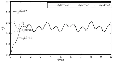
Theorem 4 is satisfied. By Theorems 2 and 4, system (6.1) is uniformly persistent and has at least one positive almost periodic solution, which is globally asymptotically stable (see Figures 2-4). This completes the proof.
0 2 4 6 8 10 12 14 16 18 20
0.1 0.2 0.3 0.4 0.5
↓
x↑1(t) x
2(t)
↓
y(t)
time t
x1
(t), x
2
(t) and y(t)
x
1(t) x2(t) y(t)
Fig. 1 Almost periodic oscillations of system (6.1)
0 1 2 3 4 5 6 7 8 9 10
0.1 0.2 0.3 0.4 0.5 0.6
← x
1(0)=0.1 ← x
1(0)=0.3 ← x
1(0)=0.6
time t
x1
(t)
x
1(0)=0.1 x1(0)=0.3 x1(0)=0.6
Fig. 2 Global asymptotical stability of state variable x1of
system (6.1)
0 1 2 3 4 5 6 7 8 9 10
0.2 0.3 0.4 0.5 0.6 0.7
← x
2(0)=0.2 ← x
2(0)=0.3 ← x
2(0)=0.7
time t
x2
(t)
x
2(0)=0.2 x2(0)=0.4 x2(0)=0.7
Fig. 3 Global asymptotical stability of state variable x2 of system (6.1)
0 1 2 3 4 5 6 7 8 9 10
0 0.1 0.2 0.3 0.4 0.5 0.6 0.7
↑
y(0)=0.1
← y(0)=0.3
← y(0)=0.7
time t
y(t)
y(0)=0.1 y(0)=0.3 y(0)=0.7
Fig. 4 Global asymptotical stability of state variable y of system (6.1)
Remark 2. Clearly, system (6.1) is with incommensurable periods. Through all the coefficients of system (6.1) are periodic functions, the positive periodic solutions could not possibly exist. However, by the work in this paper, the positive almost periodic solutions of system (6.1) exactly exist.
VII. CONCLUSION
In this paper we have obtained the uniform permanence and existence of a globally asymptotically stable positive almost periodic solution for a Watt-type almost periodic predator-prey model with diffusion and time delays. The approach is based on the continuation theorem of coinci-dence degree theory, the comparison theorem and Lyapunov functional. And Lemma 2 in Section 2 and Lemmas 2.3-2.4 in [22] are critical to study the permanence and the existence of positive almost periodic solution of the biological model. It is important to notice that the approach used in this paper can be extended to other types of biological model such as epidemic models, Lotka-Volterra systems and other similar models of first order [47-48]. Future work will include mod-els based on impulsive differential equations and biological dynamic systems on time scales.
ACKNOWLEDGMENT
The authors would like to thank the reviewer for his constructive remarks that led to the improvement of the original manuscript.