Transient stability analysis of integrated ac and dc power systems

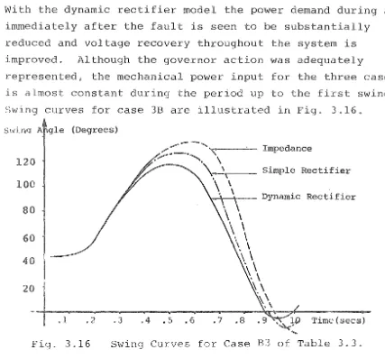
AC AND DC POWER SYSTEMS

A thesis

presented for the degree of

Doctor of Philosophy in Electrical Engineering

in the

University of Canterbury, Christchurch, New Zealand

by

K.S. TURNER B.E. (HONS), M.E.

CONTENTS Page

) List of Principal Symbols Abstract

viii xi xii Acknowledgements

CHAPTER 1 INTRODUCTION 1

CHAPTER 2 ELEMENTS OF TRANSIENT STABILITY ANALYSIS 2.0 2.1 2.2 2.3 2.4 INTRODUCTION

STEADY STATE STABILITY TRANSIENT STABILITY

MULTI-MACHINE TRANSIENT STABILITY MODELLING FOR TRANSIENT STABILITY

2.4.1 Network Representation 2.4.2 Synchronous Machine Model 2.4.2.1 Algebraic equations 2.4.2.2 Differential equations 2.4.3 Speed Governor

2.4.4 Automatic Voltage Regulator 2.4.5 Loads

2.5 COMPUTATIONAL CONSIDERATIONS 2.6 SUMMARY

STUDIES 5 5 6 8 10 11 12 13 13 15 16 16 17 18 20

CHAPTER 3 MODELLING RECTIFIER LOADS 21

3.0 INTRODUCTION 21

3.0.1 Model Application 22

3.1 BASIC RECTIFIER MODEL 23

3.1.1 Commutation Reactance of Parallel

Bridges 24

3.1.2 Basic Assumptions 26

3.1.3 Basic Converter Equations 27

3.1.4 Per Unit System 28

3.1.5 Sequential Algorithm Formulation 29

3.1.5.1 Rectifier solution 32

3.2 DYNAMIC DC LOAD REPRESENTATION 33

3.2.1 Implicit Integration for Dynamic

DC Loads 34

3.2.2 Limitations of the Sequential Algorithm

3.2 3 ~odel Limitations

3.3 ABNORMAL MODES OF OPERATION 3.3.1 Mode Classification

37 37 38 39 39 3.3.2 Equations for Abnormal Operation

3.4 UNIFIED ALGORITHM

3.4.1 Algorithm Proposal

3.4.2 Formulation of Equations for Normal Operation

3.4.3 Formulation of Equations for Abnormal Operation

3.4.4 Programme Implementation

41

43 44 3.4.4.1 Calculation of initial conditions 44 3.4.4.2 Choice of operating mode 46

3.4.4.3 Control specification 47

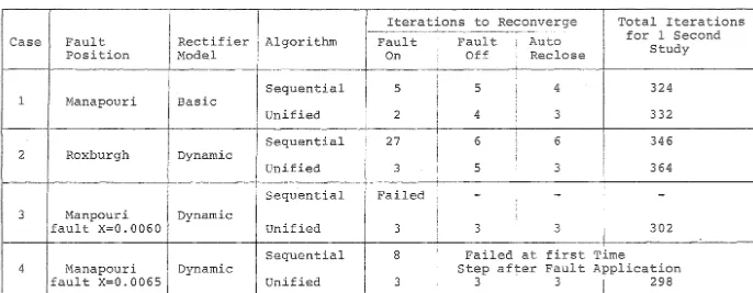
3.5 COMPARISON OF SEQUENTIAL AND UNIFIED

ALGORITHMS 47

50 3.6 RESULTS

3.6.1 System Studied

3.6.2 Discussion of Results 3.6.3 Rectifier Performance 3.7 CONCLUSIONS

CHAPTER 4 DERIVATION OF TRANSIENT STABILITY COMPATIBLE EQUIVALENTS FROM TRANSIENT CONVERTER SIMULATION WAVEFORMS

50 52 55 56

58

4.0 INTRODUCTION 58

4.1 TRANSIENT CONVERTER SIMULATION CONCEPTS 59

4.1.1 Formulation of Equations 60

4.1.2 Solution and Results 61

4.2 CONVERTER MODELLING FOR TRANSIENT

STABILITY 64

4.2.1 Transient Stability Requirements 64

4.2.2 Choice of Variables 65

4.3 ANALYSIS OF TRANSIENT CONVERTER SIMULATION WAVEFORMS

4.3.1 Effect of Modulation

4.3.2 Effect of Frequency Mismatch 4.3.3 Fourier Transforms of Periodic

68

70

71

Waveforms with Noise 72

4.3.3.1 Spectral leakage reduction 74

4.3.3.2 Choice of window 76

4.3.3.3 Mainlobe width limitation 77 4.3.3.4 Algorithm to overcome mainlobe

width limitation 77

4.3.3.6 Significance 9f spectral leakage in TCS waveforms 4.4 ALTERNATIVE TO SPECTRAL ANALYSIS

4.4.1 RMS Approximation for Voltage 4.4.2 RMS Approximation for Power 4.5 CONCLUSIONS

79 80 81 82 84

CHAPTER 5 MODELLING DC LINKS WITH TRANSIENT

CONVERTER SIMULATION INPUT 86

5.0 INTRODUCTION 86

5,1 QSS MODEL FORMULATION 86

5.1.1 Choice of Algorithm 87

5.1.2 Per Unit System 88

5.1.3 Quasi-Steady State Equations 89

5.1.3.1 Control equations 91

5.1.3.2 Series bridges 93

5.1.3.3 Including filters in the DC

link model 93

5.1.4 DC Link Control 94

5.1.4.1 Modification of control

characteristics 95

5.1.4.2 Implementation of control

mode changes 96

5.1.5 Calculation of Initial Conditions 97

5.1.6 Algorithm Performance 99

5.1.7 Programme Options 99

5.2 INCLUSION OF TRANSIENT CONVERTER

SIMULATION RESULTS 100

5.2.1 Solutions at the Link Node Using

TCS Input 100

5.2.2 Alignment of TCS Input with TS 102 5.2.3 Interactive Coordination Between

Programmes

5.2.4 System Equivalents for TCS 5.2.4.1 Obtaining time variant

equivalents

5.2.4.2 Algorithm for simultaneous fault and link solution 5.2.4.3 Algorithm tests

5.3 CONCLUSION

104 108

108

CHAPTER 6 STUDIES WITH COMBINED. TCS AND QSS DC LINK MODELS

6.0 INTRODUCTION

6.0.1 System Studied

6.0.2 Disturbances Examined 6.1 RECTIFIER AC SYSTEM FAULT

6.1~1 The Effect of Time Variant Equivalents

6.1.2 Comparison of Results

6.1.2.1 Differences in voltage and reactive power

6.1.2.2 Differences in real power 6.1.2.3 Coincidence at TCS end points 6.1.3 Approximations for TCS Equivalents 6.2 INVERTER AC SYSTEM FAULT

6.2.1 Fault Representation Using TCS Equivalents

6.2.2 Low Voltage Mismatch 6.2.2.1 Second iteration 6.2.3 Comparison of Results

6.2.3.1 Differences in voltage and reactive power

6.2.3.2 Differences in real power 6.2.3.3 Coincidence at TCS end points 6.2.4 Approximations for TCS Equivalents 6.3 DC FAULT STUDY

6.3.1 Link Performance During Fault 6.3.2 Matching QSS Restart with TCS 6.3.3 Termination of TCS

6.3.4 Comparison of Results

6.3.4.1 Recifier reactive power response 6.3.4.2 Differences in real power

6.3.5 Approximations for TCS Equivalents 6.4 CONCLUSION

CHAPTER 7 TRANSIENT STABILITY IMPROVEMENT USING DC LINK CURRENT SETTING CONTROL

7.0 INTRODUCTION

7.1 BASIC PROPOSAL FOR TRANSIENT STABILITY IMPROVEMENT

7.1.1 First Swing Stability Improvement

7.1.2 Full Damping Coritrol

7.1.3 Short Term DC Current Overload 7.2 POSSIBILITIES FOR TRANSIENT STABILITY

IMPROVEMENT

152 152

153

7.2.1 Classification of Systems 153

7.2.2 System for Study 155

7.3 THE EFFECT OF REALISTIC MACHINE MODELS 156

7.3.1 Summary of Results 156

7 3.2 Discussion 158

7.3.3 Effect on P-6 Curve 160

7.3.4 The Influence of Fault position 162

7.4 FACTORS AFFECTING TRANSIENT STABILITY

IMPROVEMENT 162

7.4.1 Magnitude of DC Current Increase 164

7.4.2 Period of DC Current Increase 167

7.4.3 DC Link position in the Network 168

7.4.4 Fault Resistance 169

7 4.5 Rate of DC Current Increase 170

7.4.6 Summary of Results 171

7.5 RESULTS WITH REALISTIC SYSTEMS 172

7.5.1 Two Generator SI System Equivalent 172

7.5.2 Full SI System 174

7.5.3 Full NZ System 174

7.6 CONSIDERATION OF FULL DAMPING CONTROL 177

7.6.1 Discussion of Controller 177

7.6.2 Results 178

7.7 ALTERNATIVE TS IMPROVEMENT SYSTEMS 180

7.7.1 Inverter End TS Improvement 180

7.7.2 DC Link Power Reversal 180

7.8 TRANSIENT CONVERTER SIMULATION RESULTS 182

7.8.1 Rectifier End Fault Case 184

7.8.2 Inverter End Fault Case 187

7.8.2.1 First Simulation 189

7.8.2.2 Second simulation 189

7.8.3 DC Link Reversal 191

7.9 CONCLUSION 194

CHAPTER 8 CONCLUSION 196

CURRENTS IN ABNORMAL MODES

APPENDIX A2 NEWTON-RAPSON SOLUTION METHOD

APPENDIX A3 FUNDAMENTAL EQUATIONS OF FOURIER ANALYSIS AND CONVOLUTION

APPENDIX A4 EFFECT OF FREQUENCY MISMATCH BETWEEN TCS AND TS PROGRAMMES

APPENDIX AS CONVERSION OF TCS SAMPLES TO A FORM SUITABLE FOR USE IN AN FFT

APPENDIX A6 DATA FOR THE NEW ZEALAND PRIMARY GENERATION AND 220KV TRANSMISSION NETWORK

APPENDIX A7 DATA FOR TS IMPROVEMENT IN A RECTIFIER AC SYSTEM - CASE 1 OF TABLE 7.1

APPENDIX A8 DATA FOR TS IMPROVEMENT IN AN INVERTER AC SYSTEM - CASE 4 OF TABLE 7.1

APPENDIX A9 DATA FOR TS IMPROVEMENT USING DC LINK POWER REVERSAL - CASE 2 OF TABLE 7.1

APPENDIX A10 PAPER PUBLISHED IN TRANS. IEEE, VOL.

205

207

209

212

213

214

219

221

223

PAS-99, NO.1, JANUARY/FEBRUARY 1980 225

APPENDIX All PAPER PUBLISHED IN PROC. lEE, VOL. 127,

PT.C, NO.5, SEPTEMBER 1980 234

APPENDIX A12 COMPUTATION OF AC-DC SYSTEM DISTURBANCES - PART I INTERACTIVE COORDINATION OF

GENERATOR AND CONVERTER TRANSIENT MODELS 237 APPENDIX A13 COMPUTATION OF AC-DC SYSTEM DISTURBANCES

- PART II DERIVATION OF POWER FREQUENCY VARIABLES FROM CONVERTER TRANSIENT

RESPONSE 246

APPENDIX A14 COMPUTATION OF AC-DC SYSTEM DISTURBANCES

THE AUTHOR

The author was born in New Zealand, in 1950 and began 'undergraduate studies at the University of Canterbury in 1969

as a bursar with N.Z. Electricity. He completed a B.E. (Hons) degree in 1972 and an M.E. degree the following year. In early 1974 he joined the Dunedin staff of N.Z. Electricity and was responsible over the next 3 years for the installation and commissioning of Southward transmission on the N.Z. HVDC Link. During this time he was also involved in developing partial discharge testing for evaluating the aged condition of

generators and in transient fault location on AC lines.

LIST OFl?RINCIPAL SYMBOLS

For convenience the symbols used throughout this thesis are defined below. In some cases, symbols have alternative meanings but if there is any ambiguity of meaning this is clarified in the text or diagram.

Symbols

I

V

R

x

X" L

C

S

P

Q

H

Current Voltage

Synchronous Machine Field Voltage Admittance

Resistance Reactance

Commutation Reactance

Synchronous Machine Transient Reactance Synchronous Machine Subtransient Reactance Inductance

Capacitance Complex Power

Real Power Reactive Power

Inertia Constant of Rotating Machine

T' T'

qo' do Synchronous Machine Transient Open C~rcuit Time Constant

Til T"

qo' do Synchronous Machine Subtransient Open Circuit Time Constant

Vd DC Voltage

Id DC Current

VLlL Thevenin Source Voltage

E~ Converter Fundamental AC Terminal Voltage I~ Converter Fundamental AC Terminal Current Zth

_{L1L :}

a Converter Delay Angle

u Converter Commutation Angle

o

o

y Converter Extinction Angle

h Integration Step Length

T Period of Power System Frequency

W Angular Frequency

x

SP

j

f (x)

x x*

[

.;

f

E

a>b a <b ++

x

Derivative of x with cos x

+

Complex Operator Function of x

Complex Variable x Complex Conjugate of x Matrix or Vector

Square Root Integration Summation

a greater than b a less than b

Fourier Transform Pair Convolution

Subscripts

a TCS Capacitive Nodes

t to Time

S

o

r TCS Resistive Branches k TCS Converter Branches r,m Real and Imaginary Parts

r,i Rectifier and Inverter Variables

d,q Direct and Quadrature Axis Synchronous Machine Variables

Abbreviations

N. Z.

S.1.

N.1.

p.u

New Zealand

HVDC TS TCS AVR DC AC FFT msec cosh cos sin rms

High Voltage Direct Current Transient stability

Transient Converter Simulation Automatic Voltage Regulator Direct Current

Alternating Current Fast Fourier Transform millisecond

hyperbolic cosine cosine

sine

ABSTRACT

This thesis describes the development of accurate models for representing power system converter loads in Transient Stability analysis.

An accurate load model is developed for rectifier loads, such as smelters and chlorine plants, in which all modes of rectifier operation are accounted for and the dynamics of the DC load represented.

The limitation of representing HVDC links with a Quasi-Steady State model are recognized and an alternative method is developed which uses interactive coordination between a transient converter simulation programme and a mUlti-machine transient stability programme. The algorithm provides an accurate AC system model for transient converter simulations and an accurate DC system model for transient stability analysis.

Case study results are presented which show the

ACKNOWLEDGEMENTS

I would like to express my sincere thanks to my supervisor, Dr. C. P. Arnold, and my co-supervisor Professor J. Arrillaga for their guidance, encouragement and friendship throughout my research.

I also wish to acknowledge the generous cooperation and interest of my post-graduate colleagues, especially Bruce Harker and Doug Heffernan, in the many stimulating discussions we had as 'sparring' partners.

Special recognition is due to New Zealand Electricity for its wholehearted support of my work. I thank NZE for supporting me as a Power Fellow, for the draughting and

technical expertise freely given by the Christchurch District Office and for the generous financial assistance provided to my supervisors for paper presentations overseas. In particular

I thank Mr. C.V. Currie and Dr. P.S. Barnett for their cooperation.

I acknowledge a special debt to my wife Brenda for her unwavering encouragement, patience and faith.

IDA good wife. who can find?

She is far more precious than jewels"

CHAPTER 1 INTRODUCTION

During the past two decades, HVDC links have been established as competitive and attractive alternatives to AC transmission and this is evidenced by the number of HVDC

schemes currently in operation or under construction. The prime motivation for their development has been large scale electric energy transport but, because of their easily

controlled power transfer, HVDC links have demonstrated a significant stabilising influence in AC power systems

(Pacific Intertie, Nelson River) . There is now a growing trend for HVDC links to be used where system stability is the primary consideration. (Eel River, CU Project, Square Butte) .

During th~ development stages of HVDC links, system planning was accomplished using small scale physical models. However such models lack flexibility in being able to change system parameters or represent large AC systems. with the advent of the modern digital computer, attempts were made to overcome the limitations of physical models using transient simulation in which the valves of each bridge are explicitly modelled. (Hingorani and Hay 1966, 1967). This method allows

for the non-linearities introduced by the many discrete switchings taking place and was later refined to provide greater computational efficiency and flexibility. (Giesner 1971, Milias-Argitis et al 1976, Arrillaga et al 1977, 1978).

In the development of transient stability analysis the emphasis has been placed on deriving accurate models for the synchronous machines and their controllers. (Kimbark 1956) . However with the availability of sophisticated computer

programmes the complexity of system representation has

increased and i t is nowrecoqnized that inaccurate load models can lead to unrealistic system responses. (CAPS Workinq Group 1973). Moreover, although QSS models have been used for HVDC link representation in TS studies, the accuracy or applicability of such models have not been justified. It is during the

disturbances used in TS analysis that the applicability of a QSS model is questionable. The QSS model cannot predict or determine the controllability of a converter and if normal valve firing sequences are disturbed by consequential valve malfunctions the QSS model cannot be used.

The objective of this work is to improve the modelling of large converter plant for TS analysis and to establish the accuracy and applicability (or otherwise) of the QSS model. This is done using Transient Converter Simulation, (TCS) , for analysing the detailed behaviour of HVDC links.

An interactive procedure is developed here in which a multi-machine TS programme is used to provide the AC system

representation required in TCS studies. The TS programme is used to derive a reduced AC network equivalent of the AC system that is time-variant and includes the transient and sub-transient effects of the dynamically responsive elements in the system. This time-variant equivalent is used for AC representation throughout a transient converter simulation of an HVDC link. The results obtained by the TCS are in turn processed to provide equivalents which represent the behaviour of the HVDC link and which are compatible with the TS study. The TCS results are therefore used to accurately represent the DC link during the disturbance period. As soon as the link behaviour returns to a quasi-steady state form the TCS can be terminated and the TS study continued using a QSS model.

interest, (i.e. HVDC links) p while providing an accurate and

time-variant representation of the remaining parts of the system without increasing computation time.

In Chapter 2 the basic parts of a modern TS programme are reviewed. It includes both synchronous machine models and computational aspects and is based on a TS programme produced initially at the University of Manchester Institute of Science and Technology (Arnold 1976) .

In Chapter 3 a model of a rectifier load is developed in which the dynamic effects of the DC load are represented. This introduces a need to improve the solution algorithm used for including the effect of the rectifier load in the

AC network. For this purpose a unified algorithm is developed which uses the Newton-Raphson solution process for the

rectifier without degrading the convergence properties of the AC system. with the dynamically responsive DC load included in the model, the response of the rectifier during disturbances can not be represented by the normal mode

equations. The model is thus extended to account for the abnormal modes of rectifier operation.

To introduce the results of a transient converter simulation into the TS programme, so that the QSS model can be replaced during the disturbance period, i t is necessary to derive TS compatible variables from the waveform orientated data provided by the TCS. Chapter 4 discusses the assumptions and errors associated with deriving fundamental frequency TS variables from distorted, noisy waveforms and also investigates approximations which reduce the computational effort required in processing the waveforms.

The QSS DC link model is discussed in Chapter 5 and the method of interactive coordination between the TS and TCS programmes is explained. Algorithms are derived so that the time-variaht network equivalents fl)r TCS may be derived with minimal change to the TS programme.

discussed to show the limits of appiicability of the QSS model.

CHAPTER 2

ELEMENTS OF TRANSIENT STABILITY ANALYSIS

2.0 INTRODUCTION

The development of large interconnected AC power

systems as we know them today, has been dependent on the fact that generators operating in parallel have a natural tendency to run in synchronism. Hence many machines can be connected to feed the same network. The degree of stability with which systems operate depends on a number of factors:

i) The size of individual generators.

ii) The position of the generators in a network. iii) The strength of the transmission network. iv) The distribution of load in the network.

Disturbances in a system, such as a fault, cause an interchange of inertial energy between the generators. The result is a change in speed of each individual machine and because this change is different for each, the machines swing relative to each other (and relative to a reference machine in the system) causing synchronising power to flow. If the swing of one machine relative to the next exceeds a certain limit, synchronism is lost, and the machines no longer continue to operate together, resulting in a collapse of the system.

The investigation of the ability of a system to remain in synchronism after a fault is known as Transient Stability Analysis. This problem has been the subject of thorough investigation since about 1920. until the advent of the modern digital computer, calculations were made laboriously by hand using many simplifications to avoid complexity.

The purpose of this chapter i's not to review the many approaches to TS analysis as they are at present. The

intention is to present the fundamentals of TS analysis and to give an overview of a modern TS programme. This overview is based on a TS programme developed by Dr. C.P. Arnold and used extensively in conjunction with the modelling of

converters throughout this work.

2.1 STEADY STATE STABILITY

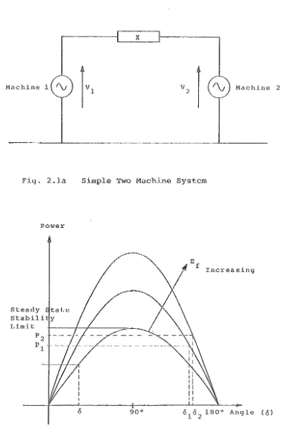
During normal steady state operation of a power system, the system load is undergoing constant and relatively small fluctuations. These fluctuations cause small deviations from constant frequency which are corrected by a change in the power output of the generators, by governor action. The power transfer between the two machines of Fig. 2.1, for example, can be described by equation 2.1.

V_IV₂

X sin <5

=

where <5 is the phasor angle between voltages VI and V

2, or the electrical angle between the rotors of the two machines. The variation of P

12 with <5 is illustrated in Fig. 2.1b. As load variations increase the power demand from a generator, the rotor angle increases to meet the demand. Figure 2.1b shows the maximum power which can be transmitted between the two machines is reached when <5

=

power delivered decreases, and the machines lose synchronism. The steady state stability limit can be increased by decreasing the transfer impedance. This is fixed for any given system and can only be decreased by the addition of more lines or transformers to strengthen the system. The

limit can also be increased using an automatic voltage

regulator (AVR) to increase VI or V2" If the AVR is used to make excitation a function of power output then the steady state stability limit can exceed 90° As illustrated ln

Machine 1

Fig. 2.la

Power

steady tate Stabili y Limit

P 2

PI

x

Machine 2

Simple Two Machine System

E

f

Increasing

increased, as

°

f , modifying the P-cS curve. In normal system operation generators are generally operating well below their steady state stability limit with angles ranging up to 40°.

2.2 TRANSIENT STABILITY

Slow variations of load can be compensated by governor action. A sudden increase in load cannot be

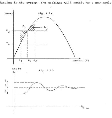
compensated for immediately, and during the interim period the extra energy taken by the load comes from the stored inertial energy of the system machines. The result is an oscillation in the rotor angles and, provided there is some damping in the system, the machines will settle to a new angle.

Power Fig. 2.2a

Angle (0)

Angle

Fig. 2.2 b

Time

Figure 2.2aillustrates the effect of a sudden electrical load increase, from PI to P2 for a single generator feeding into an infinite bus. The deceleration of the machine (due to the electrical power output exceeding the mechanical power

input) causes an angle increase to

°

2 but at this point i t is still decelerating. The machine swings to angle

°

3 and, without damping, areas Al and A2 would be equal. with damping the machine settles to a new operating point at 02. The response of the angle with time is illustrated in Fig. 2.2b.

The generator will remain transiently stable provided area A2 can always be equal to or larger than AI. This is known as the equal area criterion (Kimbark 1948). The transient stability limit is reached when A2 equals Al

but cannot increase further as is the case in Fig. 2.3. If the machine swings beyond

°

3 then stability will be lost. Power

0:;> 0₃ Angle (0)

Fig. Transient Stability Limit.

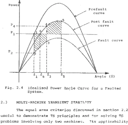
When a fault occurs in the system the power angle curve is instantaneously altered. Refering to Fig. 2.4, the output power drops from PI to P2 and the machine accelerates (due to excess mechanical power) .

At 3 the fault is cleared and a post fault

P-o

provided damping is present, it settles to a new steady state angle of 0

Powe

P

2 -

-Prefault curve

curve

Fault curve

Angle (0)

Fig. 2.4 Idealised Power Angle Curve for a Faulted System.

2.3 MULTI~MACHINE TRANSIENT STABILITY

The equal area criterion discussed in section 2.2 is useful to demonstrate TS principles and for solving TS

problems involving only two machines. Its applicability is limited for any more than two machines.

One of the early approaches to solving the multi-machine stability problem involves a point by point method of solving the differential swing equations. Once the

angular position is obtained at a given step the network is solved to determine a new electrical power for the solution of the swing equation at the next step. This method is extremely laborious, synchronous machine representation was in most cases limited to a voltage behind reactance and the method on its own could only be applied to small systems. As the size of the network increases the network part of the

solution becomes increasingly more difficult.

This problem is overcome by the use of an AC network analyser. The network analyser is a scaled physical model of the system which, when given the relative machine angles

around the network for the next point of the swing curve.

with the advent of the digital computGr the alternating solution of the differential and network equations was

implemented entirely on the computer, eliminating the need for any hand calculations. The complexity of the machine model could be increased and the system size was only limited by the amount and speed of the computing time available.

A number of different algorithms were developed to improve the efficiency of the computation, the most

significant one being reported in 1972, (Dommel and Sato 1972) in which the differential and network equations were solved simultaneously. This new algorithm eliminated

interface errors which occur when the differential and network equations are solved alternately,as with the earlier

algorithms. This was done using an implicit rather than an explicit integra~ion method allowing the differential

equations to be algebraized, included in the network algebraic equations and solved simultaneously.

The trapezoidal rule is numerically stable, (Law 1972) , and can be used with step lengths greater than the smallest time constant of the system,without instability or excessive errors. This allows detailed representation of machines, their AVR's and governors, induction motors and non-impedance loads without affecting the numerical performance of the

programme. The models used for the various system elements are well known and their operational features will be presented without further justification.

2.4 MODELLING FOR TRANSIENT STABILITY STUDIES

The conditions throughout a network at a given step of a TS study are defined by:

i) A set of steady state algebraic equations of the network, loads and rotating machines, i.e.:

(X,Y)

=

Y == f(X,Y,t) ( 2.3)

where X are the non integrable variables which depend on a set of algebraic constraints (examples of which are busbar voltages and electrical powers)

Yare integrable variables which depend on a set of time variant restraints (i.e. rotor angles or internal emf's)

and and

F

When there is a sudden disturbance to the system, variables X show a discrete change following the disturbance while variables Yare continuous as a discrete change in them is not possible by definition.

The solution of the TS problem using implicit

integration involves the algebraization of equation 2.3 into the same form as equation 2.2 and subsequent solution of equation 2.2.

2.4.1 Network Representation

Lines, transformers and cables can be represented by a combination of series and parallel impedances, commonly in an equivalent 1T network as illustrated in Fig. 2.5.

For a line, Yab represents the transfer impedance and Y the shunt susceptance. i.e.:

aa

b

-

Y ::::: _{(2 .4)}

ab R

+

₌

bb ::::: -jB (2.5)

aa _/2

The same applies for nominal tapped transformers and cables. For an off nominal tap transformer the elements are modified by the tap position.

% off nominalu then:

If the tap position, T u is given in

a

₌

and Y

=

ab t

Y (a 2 a)Y

ab ( 2 .8)

=

-aa t Y

bb

=

-

t

In a nodal admittance formulation of the network, equation 2.2 is of the form:

[I]

=

where [11 is a vector of injected currents I [Y 1 the network

admittance matrix and [V] the vector of nodal voltages. Admittances Y.. form diagonal elements of

11

i~j form off diagonal elements of [Y]

2.4.2 Synchronous Machine Model

[Yl and Y .. ,

1J

The most important model and one which affects TS results significantly is that of the synchronous machine. The model is made up of both algebraic and differential equations.

2.4.2.1 Algebraic equations - In a conventional d-q reference frame of representation the basic equations

describing a synchronous machine are:

R

a

··x

(2.11) E - V

This is a steady state (synchronous) description but is equally valid for transient and subtransient behaviour by replacing synchronous reactances by transient or subtransient values and the voltage behind synchronous reactance by

transient or subtransient respectively. i.e., for increasing degree of detail from left to right:

x

q q q

(2.12) E ~ ED ~ E"

To interface the d-q model to the network frame of reference a transformation is required, i.e.:

- j (~ - 6)

( I

+

=

d + j I ) e 2

r m q (2.13)

In the network frame of reference the machine model can be summarised by:

I

₌

fict

(E

- \7)

where Y

fict (R j(xd + x )/2)/(R 2

XdXq) (2.15)

=

-

a q a

I

=

(E

- *

sal sal

Y

=

d

-

sal q a

The Norton equivalent of equation (2.14) is illustrated

in Fig. 2.6.

-v

Terminal Busbar

In the nodal admittance formulation of equation 2.2 the admittance Y

fict can be included directly into the

_-

f · t.E become

sa lC

part of the vector of nodal injected currents. Since I

sal is a function of the unknown bus voltage,

v ,

2.4.2.2 Differential ions - The differential

equations for the machine are related to two different effects: i) The electro-mechanical response of the machine.

ii) The dynamic behaviour of electrical characteristics. The electro-mechanical response is described by the well known swing equation, here given as two first order equations:

w

=

o

=

where P is the turbine shaft power,

m P e

(2.18)

(2.19) is the electrical output power, D

a is a damping factor related to the change in positive sequence flux,

w

o is the nominal and w the

actual machine speed. The dynamic response of the flux linkages is governed by the transient and subtransient open circuit

time constants. state, by:

Their effect is introduced,in the transient

E'

d

E' q

=

=

[ (x - Xi) I - E i ]

IT

q q q d qo [E

f - (xd - x') d I d - E q I ]

I

E"

=

IT"

d d q q q d qo

E"

q

=

IT"

(2.20) (2.21)

(2.22)

saturation, which affects only the mutual rotor-stator flux, modifies equations 2.14 and 2.20 to 2.23. Although saturation is a very nonlinear characteristic, linear approx-imations can be applied with acceptable accuracy, (Olive 1966),

us~ng saturation factors to preserve the linearity of the

equations. As saturation cannot be easily presented briefly the details will be omitted.

2.4.3 Speed Governor

without a governor model, the mechanical power, P , of m equation 2.18 is assumed to remain constant. This assumption is rea~onable when only first swing transient stability is being examined since governor action is relatively slow.

For longer term studies governor action can have an appreciable affect on the shaft power and subsequent system response after the first swing. Governor response can also indicate trends in the longer term power-frequency balance problem.

The governor is normally modelled by a set of

differential equations obtained from the transfer functions of a functional block diagram. The equations become part of equation 2.3. Standard governor models have been developed,

(IEEE Committee Report Feb. 1973) and are widely used in many TS programmes. Separate documentation is unnecessary here. The present TS programme incorporates a range of models from a simple, to a fully detailed representation of both hydro and steam turbine governors.

2.4.4 Automatic Voltage Regulator

The purpose of the AVR is to control the terminal voltage, V, of the generator to a fixed value. This is done by monitoring the terminal voltage and varying the excitation voltage, Ef, of equation 2.21. This provides a secondary change to the rotor-stator flux linkages apart from their natural response given by equations 2.20 to 2.23.

2.4.5 Loads

Most commerical and domestic loads can be represented as constant impedances. With this representation a nominal impedance is calculated, based on the initial power and

voltage obtained from a loadflow. This impedance can be

included directly into the admittance matrix of equation 2.10. Non impedance type load models can be used for specific applications where the impedance load characteristic is not representative. In such cases, constant current and constant power characteristics, as illustrated in Fig. 2.7, can be

used.

I

Constant Power

Constant

Impedance

Nominal V Voltage

Fig. 2.7 Non Impedance Load Characteristic.

This type of load is included in the TS programme by

calculating the nominal admittance of the load and modifying the characteristics by calculating an injected current which represents the deviation of the chosen characteristic from an impedance. The injected current is added to the nodal current vector, [I] p of equation 2.10. Special precautions

have to be taken to ensure that abnormally large injected currents, which may upset the numerical stability of the programme, are not required to produce the chosen

Special industrial induction motor loads can also be represented with a detailed induction motor model developed recently, (Arnold et al 1979).

The functional relationships between the network, synchronous machine, governor, AVR and loads, in TS

modelling, are illustrated in Fig. 2.8.

2.5 COMPUTATIONAL CONSIDERATIONS

The major part of the computational effort used in TS studies is required in the solution of equation 2.10. The size of matrix [YJ goes up as the square of the number of buses in the system. One of the attributes of [YJ is that i t is very sparse, i.e., for a 100 bus system only about 4% of the 10,000 elements in [YJ are non zero.

However solution of equation 2.10, by computing the inverse of [YJ explicitly, i.e.

[V]

=

results in a full matrix requiring much greater storage and processing. Because of the iterative nature of the TS problem and the number of steps for a complete run, computation methods requiring [y]-l explicitly, become prohibitive for large systems, even on modern very fast computers.

A highly efficient algorithm has been developed, (Zollenkopf 1970), for the direct solution of sparse net-works without the formation of [y]-l explicitly. This method, bifactorisation, is very fast as i t preserves the

sparsity of the original matrix and only processes non zero elements. The method is based on the technique of

Gaussian Elimination in which Y is reduced to a matrix, ~,

U, in upper triangular form, i.e.

[I]"

=

It is thus possible to solve for [V] by backward

substi tution. Using this approach, [Y] can be represented by its upper and lower triangular matrices and a unit

~

'.":

Equotion5

Turbine Clovernor

Equations

f - - -... mo-I Machine Electrical

Equations

Ef

Pm _SynchronoU5

Machine Mec.hanical

1r.

---I1

- - - - t - - - - '

S

Differential Equation~

Id,Iq, Ro

Pe

I

I I I I

J<.d: I<.q,' I

[v]

I

[iJ

] I

I

I I

i

1- _ _ _ - '

I NehNork

I I

Transformation From

D-Q Reference frame to

Network Referenc.e Frame.

.t\\gebraic Eq,uations

Fig. 2.8 Functional Relationships of a T.S. Model (in the Transient State)

i-'

~

[Y]

=

-

-and [I] :::: [L] [D] [U] [Vj (2.27)

In this form [L]

=

The modified vector, [I]" f can be obtained by forward

substitution on [Lj and many solutions for [V] can be obtained without re-triangularisation provided [Yj remaj.ns unchanged. Re-triangularisation is therefore only necessary when the system is subjected to a topological change.

If [Y] is sparse then [L] and [U] are also likely to be sparse and ordered elimination uses highly

efficient sparsity programming to store and process only the non zero elements. During the eli~nination, pivots are

selected to obtain maximum preservation of the sparsity of the arrays. The elimination is initially simulated, to determine the pivot ordering in advance and to organise the subsequent eliminati~n processing so that i t can be executed very rapidly without storage being wasted.

The algorithm, outlined above, has been implemented in the present TS programme. Its performance has proved to be highly successful making the programme one of the fastest available at the present time.

2.6 SUMMARY

The basic features of a modern TS programme have been presented. Considerable effort has been spent on the

development of TS analysis in the past as evidenced by its prominence in the literature. A lot of effort has been

spent on improving modelling techniques to make the programmes a more effective tool for power system analysis. Most of the material presented here can be found in the literature but as a basic reference the author would refer the reader to

CHAPTER 3

MODELLING RECTIFIER LOADS

3.0 INTRODUCTION

Transient stability is generally regarded as a problem of keeping dynamic power system elements in synchronism.

Because of this, the traditional emphasis in developing models for TS analysis. has been placed on generator

representation and efficient computational techniques for digital computer implementation. It is only relatively

recently that importance has been attached to load modelling and the contribution which loads make to system damping.

(Concordia 1975). Emphasis has been placed on induction motor response (Brereton et al 1957, Iliceto and Capasso 1974, Hakim and Berg 1976) and investigations of composite load dynamics.

(CAPS Working Group 1973.) Little consideration has been given to large rectifier loads.

Rectifier loads with high power ratings and

sophisticqted power electronic control have become common in power systems.

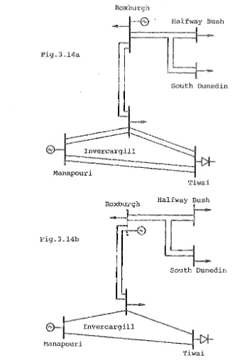
Figure 3.1 illustrates the primary transmission system of the South Island, (SI) p of New Zealand which includes a

large aluminium smelter and DC link. DC links require

separate treatment and are considered later in this work. The rectifier load at the smelter represents some 13% of the

total SI installed capacity. Since this load is constant i t can represent up to 50% of the SI load during periods of light load. The size of this load is sufficiently large to affect the dynamic response of the system and an accurate

representation of i t is therefore important.

In this chafter an accurate representation for

rectifier loads is developed. The model includes the dynamic effects on the DC side of the rectifier and is extended to include abnormal modes of operation during large disturbances. The model is therefore accurate for the wide range of conditions that may prevail during TS analysis. A second (unified)

Kikaw'a

Tekapo B

Twizel Ohau A

264 MW

Ohau C

212 MW

Ohau B

Stoke

Islington

W

itaki

Livingston

320 MW Half Way _Bush

tv

South Dunedin

)l~~========~R~O~X~b~U~r~g~h~==========i===n

Manap0l:;:ur i

~t===================================~~~~~Tiwai

Fig. 3.1 New Zealand South Island Primary System

programme which showed considerable deterioration in

convergence when the dynamic DC load is modelled usiny the more conventional sequential algorithm.

3.0.1 Model Application

Rectifier loads utilise a number of control methods, i.e., diode or thyristor elements in full or half wave rectification. Although the particular load considered in this work is an

aluminium smelter the model is applicable to any large rectified load (such as chlorine plants) by specifying the correct input parameters.

control affects diode conduction in ~n identical manner to a normal thyristor bridge (Fuji Electric 1972) but the equivalent of the delay angle has a much more limited range.

is illustrated in Fig. 3.2. Flux Density

+B

-B

m m _I

~

Control Current

Co

~

I

a u

This action

Saturable

conduct~on

Fig. 3.2 Saturable Reactor Control of Diode Conduction. The thyristor controlled biasing voltage maintains the series saturable reactor at a high impedance until the

forward voltage is high enough to cause saturation of the reactor. During this period commutation cannot take place and the reactor absorbs the forward voltage equivalent to

the shaded area in Fig. 3.2. As soon as saturation is reached the reactor impedance drops and normal commutation takes

place.

The range of control, exerted by the saturable reactors at the Tiwai smelter is equivalent to a delay angle range from 3 to 20 degrees.

3.1 BASIC RECTIFIER MODEL

Large rectifier loads generally consist of parallel

and/or series connected 3 phase full wave bridges. For smelter applications converters are paralleled on the DC side to

achieve the high currents required for smelters. For simplicity of modelling i t is possible to reduce these

3.1.1 Commutation Reactance of Parallel

Figure 3.3 is a single line connection diagram of one potline at the Tiwai smelter.

System Source Voltage

1\1

System S@urce Im eaance

x

220

kv 220/33 kv

33kv/0.76kv

E _Ia Ia

r

l 1 2

E Ia

r

2 3 Va

I

Rectifier Unit

I

x

i

-L ____ - _ I 21--,

Fig. 3.3 Single Line Connection Diagram for one Potline at Tiwai Smelter.

The source voltage for one of the bridges is defined as the voltage appearing on the DC line during the period when no commutation is taking place, i.e. the purely sinusoidal voltage nearest the rectifier. (Uhlmann 1975) . For the case illustrated in Fig. 3.3, this would be the system source

voltage. If filters are connected on the 220kv or 33kv bus's then the voltage at the filter bus would become the source voltage since, ideally, i t would be purely sinusoidal. The commutation reactance is defined as the reactance between the source voltage and the converter.

When considering a single bridge (bridge 1) of Fig. 3.3, the commutation reactance,

However with multiple bridges which' are phase shifted in relation to each other, the high pulse number of the system means that the voltage at the 33kv bus is essentially

sinusoidal and can therefore be considered as the source v'ol tage of the system. In this case the commutation reactance of a single bridge becomes:

=

Although the network reactance does not contribute to the commutation reactance, i t still affects the source voltage in the normal AC manner by the regulating effect of an AC current through an impedance.

Since the 4 bridges are under the same controller i t is assumed that:

E

₌

₌

₌

₌

rl r2 r3 r4 r ( 3 .3)

Idl

=

=

=

and _4Idl

₌

In this case the parallel combination of Fig. 3.3 can be modelled as a single equivalent bridge, Fig. 3.4, in which:

I LlJ!.l:a

r

x

ELQ

r

Fig. 3.4

=

V cell

Smelter Rectifier Load Equivalent.

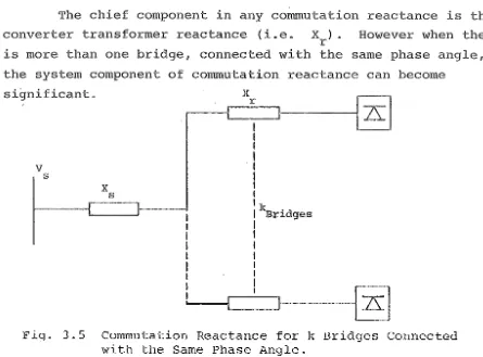
The chief component in any commutation reactance is the converter transformer reactance (i.e.

x ).

r

is more than one bridge, connected with the same phase angle, the system component of commutation reactance can become

significant

.

r

x

K

I

I

I

I

v

s I

x

s I

I

I k 'd

I Br~ ges

I I

I I

Fig. 3.5 Commutation Reactance for k Bridges Connected with the Same Phase Angle.

Referring to Fig. 3.5, for k bridges all with the same connection phase angles, the system reactance will be commutating k times the current of a single bridge and in this case with commutation reactance of one bridge is:

=

+

s Xr (3 .7)

This assumes each bridge is operating with the same direct current.

3.1.2 Basic Assumptions

Further assumptions are made in formulating a basic rectifier model. These are:

i) The rectifier source voltages are balanced, three phase waveforms with negligible distortion.

ii) The losses in the converter transformer are negligible.

iv) The DC current and voltage are smooth.

v) Control action affecting delay angles is considered to be instantaneous.

vi) No tap changer action takes place during or immediately after a sudden disturbance.

These assumptions are well documented and accepted elsewhere (Kimbark 1971) and will not be justified separately in this work.

3.1.3 Basic Converter Equations

A number of basic equations can be derived from first principles (Kimbark 1971, Adamson et al 1960), to interrelate the variables in Fig. 3.4. The constants in the following equations are given with the source voltage, E as a

r

phase to phase quantity referred to the secondary side of the converter transformer by the tap, a .

DC voltage:

In terms of the

=

In terms of DC current:

=

aE

r

~ (cosa - coso) c

( 3.8 )

(3.9)

Using equation 3.9, the commutation angle can be eliminated from equation 3.8 to give a more convenient form for DC voltage: i.e.

=

-1T r

3X c

-1T (3.10)

Using Fourier analysis the fundamental component of AC current at the terminals of the converter transformer can be related to the DC current by:

I

r

=

16

1T

(1 /~~2a - I - 20 - j2u1

l

The expression in parentheses is cownonly equated to a

I :=

r ak 1

16

For normal operating conditions of a converter, approximated to unity with less than a 1% error. commutation angle of 600 _{the error is 4.3%.}

(3.12)

kl can be With a

An approximation for the power factor at the converter transformer can be obtained by equating real AC and DC powers across the converter: i.e.

:=

13

r r

where cP

=

e -

substituting for Ir with equation 3.12 and Vd with equation 3.8 gives

cos¢

=

2~

(3.13)

(3.14)

Using Kirchoffs laws around the DC current loop provides:

=

The above set of equations are fundamental to quasi-steady state models of converters.

3.1.4 Per Unit System

MVAb

AC

Fig. 3.6

-Per unit Definitions.

The AC terminal voltage referred to the DC base becomes:

(3.16)

The commutation reactance, given on an AC base, also has to be modified before i t can be used in the DC equation, viz:

X

c(pu)DC

=

(Vb AC]

lV

2

(3.17)

Hence equation 3.10, in terms of per unit quantities becomes:

3/2

V

=

d(pu)DC 7T aE r(pu)DC coset. 7T 3 X c(pu)DC I d(pu)DC (3.18) 3.1.5 Sequential Algorithm Formulation

[VJ _i +_l := _(3.19)

at the ith iteration.

The rectifier model is included in a similar way. From an initial loadflow a nominal bus shunt admittance Y can

o be calculated for the rectifier from:

G

_o

=

IE

12

0

r

B _o

= -

IE

12

0 r (3.21)

where E

r is the nominal AC bus voltage obtained from the

initial loadflow solution and:

s

=

+

0 0

(3.22)

Y

=

+

0 0 0

y _{is included directly into the network admittance matrix} [Y] •

0

The rectifier is solved at each iteration of the TS run and any departure from the impedance characteristic is accounted for by calculating an injected current using:

I

=

(Y

r . . 0

l n J

where Y

Y)

1

(3.23)

(3.24)

and E

r is the terminal voltage at the rectifier obtained from the previous iteration.

the current vector of equation produces a new value for E

r I

r can then be included in 3.19 which, after solution, and therefore a new rectifier state. The process is iterated to convergence as the

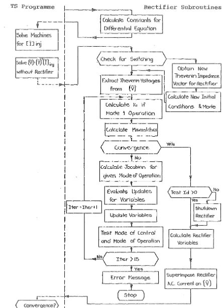
dynamic equipment and rectifier settle to a solution. algorithm is illustrated in the flow chart of Fig. 3.7.

I

1

Load flow solution

Input

Calculate

Yo

Include

it

(yJ

Begin TS Run

Solve Rectifier

to

obtain

'9

-Calcu\Qte

I

Solve

Generators

(Iin

J

Update Vector of Nodal Voltages

Test for Convergence

between suCc.essive

I te.rations.

+

End of Run?

( Exit

Iter -= Iter t I

No

3.1.5.1 Rectifier lution ~ With a given AC terminal voltage and specified control regime, a simple rectifier can be solved directly without iteration. Constant current control is normally used for smelting applications and, provided the delay angle is within its specified control range, the DC current can pe calculated from Fig. 3.8 by:

=

where A is the constant current controller gain.

"---

---

- - v

d rnln c

Slope given by

Regulator Gain (A)

I

d set

Fig. 3.8 Simple Rectifier Control Characteristic.

substituting for Vd with equation 3.15, Id can be solved for directly using:

=

with this given current the delay angle can be obtained using equation 3.10. If the delay angle is within the limits of its permissible operating range, the AC power factor can be obtained and the power flow evaluated, i.e.:

If a lies outside the range of the controller limits the control changes to constant a mode.

and 3.15 Id can be calculated by:

Using equations 3.10

=

l , ' t - V 11)/(Rd + 3X

In)

n r lml ce c

where _{aI' ' t}

lml

=

(3.28)

Protection limits and disturbance severity determine the rectifier operating characteristic.during a disturbance. Shutdown occurs if Id reaches a specified minimum, (or zero), and the existence of cell counter voltage will cause shutdown before the AC terminal voltage reaches zero.

3.2 DYNAMIC DC LOAD REPRESENTATION

The basic rectifier model outlined in section 3.1 assumes that both a and Id can change instantaneously as determined by the behaviour of the AC terminal voltage. This may be valid for some rectifier loads but data for the NZ smelter (Fuji Electric 1972) indicates that:

i) The controller time constant is of the same order as the integra tion step length of the TS programme (10 msec) .

ii) The DC load time constant is much larger and is 113 msec.

Because of the very small controller time constant i t is not necessary to model control dynamics. For a severe disturbance the rectifier is subject to a large drop in

However the time constant of 'the DC load is of the same order as the fault period itself and will modify the performance of the rectifier considerably. In order to realistically examine the effects which rectifiers have on transient stability the time constant must be taken into account.

3.2.1 Implicit Integration for Dynamic DC Loads

As soon as a reaches its limit the dynamic response of the DC current is described by:

=

cell

+

where L is the equivalent inductance of the DC load. substituting for _Vd using equation 3.10, 3.29 can be written in the form:

Id

=

i . e. Id (t)

=

-

where A

₌

1 [3Xc )

B

₌

IJ

T 'lTRd C

=

and T

=

(3.29)

(3.30)

(3.31)

(3.32)

(3.33)

(3.34)

By using the trapezoidal integration method, for any time function x (t) ,

x (t + h)

₌

2

where h is the integration step.

=

K

+

where Ka

=

(3.36)

(3.37)

(3.38)

The constants Ka and Kb can be evaluated at the beginning of each step, using the results of the previous step. The

current values of Er and cosa provide a new estimate for Id at time t+h. Since a is normally on its limit and therefore constant, i t is not required explicitly in equation 3.36 and can be absorbed in the constant K .

a

3.2.2 Limitations of the Sequential Algorithm

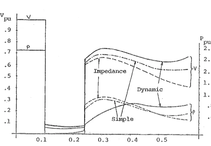
The basic rectifier model of section 3.1.5 does not depart greatly from an impedance characteristic and hence the injected current required to compensate for its

characteristic is not large. Figure 3.9 demonstrates the difference between the two characteristics.

I

r

I F.L

Impedance

0.5

Rectifier (C.C.C)

1.0 E

r

E r

Fig. 3.9 Difference between Impedance and Simple Rectifier Characteristic (for V

The rectifier characteristic 'is well behaved with the injected current tending to zero as the voltage approaches zero, as distinct from non impedance type loads, (constant current or constant power), in which the current does not drop naturally to zero at low voltage. No convergence problems

were experienced with. the basic rectifier model but non impedance type loads have created convergence difficulties when implemented in the sequential algorithm. (stott 1979) .

When the basic model is modified to account for the dynamic behaviour of the DC load, the injected current departs widely from that of an impedance characteristic during stages of the transient stability run. Immediately after a fault application the voltage drops to a low value but the injected current magnitude remains essentially the same due to the slow rate of change of DC load current. Similarly on fault

clearance, the voltage recovers sharply but the injected current remains low.

with this characteristic the sequential solution method exhibited similar convergence problems to those experienced with non impedance loads. When the fault was applied at some distance from the rectifier terminals there was no deterioration in convergence of the AC system since the injected currents required to account for the DC load behaviour are moderate. As the fault was moved towards the rectifier and the AC voltage at the rectifier terminals

during the fault decreased, the number of iterations to convergence progressively increased.

The problem appears to be due to the phase of a large injected current vector being affected by the phase variations of a small voltage vector, with successive iterations. The phase variations of the large current vector upsets the smooth convergence of the sequential algorithm.

3.2.3 Model Limitations

This led to a rapid rise in commutation angle immediately after fault application and commutation angles exceeding 60° were observed. This mode of operation is outside the valid range of the normal mode equations and to model dynamic effects i t is necessary to extend the model to represent abnormal

modes of operation. In addition, an improved algorithm is required to eliminate the convergence problems of the

sequential algorithm.

3.3 ABNORMAL MODES OF OPERATION 3.3.1 Mode Classification

The full range of rectifier operation can be classified into four modes. (Giesner and Arrillaga 1970).

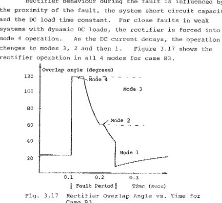
Mode 1 - Normal operation. Only two valves in the bridge are involved in simultaneous commutation at any one time, This mode extends up to a commutation angle (u) of 60°,

Mode 2 ~ Enforced delay. Although a commutation angle greater than 60° is desired, the forward voltage across the incoming thyristor is negative until either the

previous commutation is complete or until the firing angle exceeds 30°, In this mode u remains at 60° and a can range up to 30°.

Mode 3 - Abnormal operation", In this mode periods of 3 phase short circuit and DC short circuit exist when two commutations overlap. During the period there is a controlled safe short circuit which is cleared when one of the commutations is complete. During the short circuit period 4 valves are conducting.

Mode 4 - Continuous three phase and DC short circuit caused by two commutations taking place continuously. In this mode the commutation angle is 120° and the AC and DC current paths are independent.

TABLE 3.1 RECTIFIER MODES OF OPERATION

Mode Firing Angle a Overlap JIngle u

1 _{0° '" a} ~ 90° 0° < u ~ _60°

2 _0° ~ a ~ 30° 600

3 300 _{~ a}

_<-

4 300 _{~ a ~ 90}0 ₁₂₀0

3.3.2 Equations for Abnormal Operation

Equations 3.8 and 3.9 do not apply for a converter operating in mode 3. These two equations are modified for abnormal operation and become: (Kimbark 1971) .

aE r

=

l6X

where a'

=

-

0'

=

(3.39)

(3.40)

(3.41) (3.42)

An equivalent form of equation 3.10 can also be derived, i.e.:

v

=

d TI r TI d (3.43)

In mode 2 both normal and abnormal equations are valid. In mode 4, Vd

=

Equation 3.11 is only valid for modes 1 and 2 and its use cannot be extended into mode 3. As an initial