SEMI DISCRETE FORMULATION OF GALERKIN -PARTIAL ARTIFICIAL DIFFUSION FINITE ELEMENT METHOD FOR COUPLED BURGERS' PROBLEM

(1)

Available Online at www.ijpret.com

1

INTERNATIONAL JOURNAL OF PURE AND

APPLIED RESEARCH IN ENGINEERING AND

TECHNOLOGY

A PATH FOR HORIZING YOUR INNOVATIVE WORK

SEMI DISCRETE FORMULATION OF GALERKIN -PARTIAL ARTIFICIAL DIFFUSION

FINITE ELEMENT METHOD FOR COUPLED BURGERS' PROBLEM

NAJAT JALEEL NOON

Basrah University, Education College, Mathematics Department

Accepted Date: 22/10/2013 ; Published Date: 01/12/2013

Abstract: The viscous Burgers’ equation is an example of an equation that has unstable

Galerkin finite element approximation for the convection-dominated case. In this paper, a stabilized finite element method for solving coupled Burgers’ equation in 2-D is studied, the method consists of adding artificial viscosity acting only on the small scales. We consider a semi-discrete formulation, the theoretical evidence proved the stability and proved that the

error estimate is of order (ℎ ). The discretization with respect to space variables only is

applied, whereas time remains continuous. This leads to a large system of ordinary differential equations which are solved using the MATLAB function ODE45 where the numerical results are compared with the exact solution.

Keywords: Galerkin -Partial Artificial Diffusion, Error Estimate, Burgers' Equation.

Corresponding Author: NAJAT JALEEL NOON

Access Online On:

www.ijpret.com

How to Cite This Article:

Najat Jaleel Noon, IJPRET, 2013; Volume 2 (4): 1-24

(2)

2

INTRODUCTION

In recent years, Burgers’ equation have received a considerable amount of attention due to the large number of physically important phenomena that can be modeled using this equation. Some attention has been given to the convection-dominated case. Several methods have been intensively studied to remove such a drawback for this problem and relevant problem, we can summarize some of the most relevant literature. Atwell and King [1] used the Galerkin and Galerkin Least-Squares approximation for 1-D Burgers' equation with the linear feedback control law designed for the non-stabilized problem. Heitmann[5] applied subgrid scale eddy viscosity for convection dominated diffusive transport. The method consists of adding artificial

viscosity term ( , ∇ ) of orthogonal projection acting only on the fine scales, he

give a comprehensive analysis of this method, in [6] he applied this method in a finite

difference method by using an appropriate interpretation of the term ( ,∇ )≡

( ,∇ )− ( ,∇ ), where is an average over itself and its five nearest discrete

neighbors. Volkwein [10] considered upwind techniques and mixed finite elements for the steady-state Burgers' equation in 1-D to compute solutions for small viscosity parameters . Diez, Gunzburger and Kunoth [4] studied the multiscale finite element viscosity method for hyperbolic conservation laws which was applied to 1-D inviscid Burgers’ equation developed in terms of hierarchical finite element bases to a wavelet basis for a controlled adaptive resolution of discontinuities of the solution. Chan, Demkowicz, Moser and Roberts [3] applied Discontinuous Petrov-Galerkin to 1-D Burgers’ and compressible Navier–Stokes equations, they

were able to solve problems with Reynolds number up to Re =10 . Kashkool and Noon [7]

used the classical artificial diffusion for Galerkin and Galerkin-Conservation finite element methods for coupled Burgers’ problem in 2-D for the convection-dominated case. The fully discrete formulation with the backward Euler -Galerkin and Galerkin-Conservation schemes

were considered. the error estimate of these methods were of order (ℎ, ) and the

numerical results were compared with the exact solution. In this paper, we present a stabilized finite element method for solving coupled Burgers’ problem in 2-D, the method consists of adding artificial viscosity acting only on the fine scales to a variational formulation of the problem. We consider a semi-discrete formulation, we prove the stability and convergence for the approximation. The numerical solution of this method is compared with the exact solution . This paper is organized as follows. In section 2, definitions and some important theorems are given. In Section 3, we present the time-dependent modeling problem and a

weak form of 2-D Burgers’ problem and we show the continuity and −elliptic. The

(3)

3

finite element approximation, test problem and numerical results are introduced. The conclusions is shown in section 6.

2- Definitions and some important theorems

It is beneficial to mention the definitions and some important theorems which will be used frequently in the equal .

Definition 2.1 [5] For Ω ⊂ the ( , ) weighted norm of a function ∶ Ω → is defined by,

║ ║ _, = ║ ║ + ║∇ ║ .

Definition 2.2 [5] For Ω ⊂ the ( , , ) weighted norm of a function ∶ Ω → is defined

by, ║ ║ _{, ,} =║ ║ _, + ║ ║ .

The operator is a projection operator which will be discussed in section 4.

Definition 2.3 [5] Given any real number define the weighted norm ║.║_{( :( , ))} on Ω×

(0, ] to be, ║ ║_{( :( , ))} =∫ ( )_{║ ║} _.

Theorem 2.1 (Poincaré Inequality). [8] Let Ω ⊂ be a bounded domain. Then, there is

constant = (Ω), such that for any ∈ , ║ ║ _{( )}≤ ║ ║ _{( )}. (2.1)

Theorem 2.2 (Lax–Milgram Theorem).[8] Let be a Hilbert space with inner product (. , . ) and

let (. , . ) be a coercive continuous bilinear form on , and let (. ) be a continuous linear form

on . Then, there exist a unique solution ∈ to the abstract variational problem: find ∈

such that, ( , ) = ( ), ∀ ∈ .

Theorem 2.3 (Inverse Estimate). [8] On a quasi-uniform mesh any ∈ satisfies the inverse

estimate, ║ ║ _{( )} ≤ ℎ ║ ║ _{( )}. (2.2)

Abstract Results [2]

Let be a separable Hilbert space , let be a bounded symmetric bilinear form on

with the property that for some δ > 0, ( , )≥ ║ ║ , ∀ ∈ , (2.3)

and let be a trilinear form on such that there exists a constant > 0 such that

(4)

4 Remark 2.1 [5]: We shall state the following inequality which will be used frequently in this

paper, ‖ − ‖ ≤ ℎ ║ ║ , 1≤ ≤ , ≥2. (2.5)

3- Time-Dependent Modeling Problem

Consider the nonlinear time-dependent for the two dimensional coupled Burgers’ problem[11].

− є∆u+ + = , (3.1.a)

− є∆ + +v = , (3.1.b)

with boundary conditions

( , , ) = 0 × (0, ], ( , , ) = 0 × (0, ],

and initial conditions

( , , 0) = ( , ) , ( , , 0) = ( , ),

Where >0 is a viscosity constant, ⊂R with boundary ∂Ω, = ( , , ), = ( , , ),

and ∈L ( ).

The weak formulation of (3.1) is : find , ∈ = (Ω) such that:

( , ) + ( , ) + ( , , )+ ( , , )=( , ), (3.2.a)

( , )+ ( , )+ ( , , )+ ( , , )= ( , ),∀ ∈ (Ω), (3.2.b)

( ( , ,0), ) = ( , ), ( ( , , 0), ) = ( , ),

Where ( , ) = (є , ) and ( , ) = (є , ), ( , , ) = ( ,φ), ( , , ) =

( , ), ( , , ) = ( , ), ( , , ) =( , ),

The weak formulation (3.2) with artificial viscosity term ( , ∇ ) is : find

, ∈ = (Ω) such that:

( , ) + ( , )=( , ), (3.3.a)

(5)

5

Where, ( , )= ( , )+ ( , )+ ( , , )+ ( , , ),

( , )= ( , )+ ( , ∇ )+ ( , , )+ ( , , ).

Assumption 3.1:

(A1)There exists a constant such that: ≥ > 0.

We assume that the solution and of problem (3.2) satisfied the following condition

(A2) , ∈ (0, , (Ω))∩ (0, , (Ω)), , , , , , ∈ (0, , (Ω)).

Lemma 3.1: (u, ) and (v, ) given by (3.3) are continuous and V-elliptic(coercive).

Proof: 1-For continuity ,we have,

| ( , )|≤ |є( , )|+| ( , )|+|( , )|+|( , )|,

| ( , )|≤ |є( , )|+| ( , )|+ |( , )|+ |( , )|,

| ( , )|≤|є( , )|+| ( , )|+|( , )|+|( , )|,

Applying Cauchy-Schwartz inequality gives,

| ( , )|≤є║ ║║ ║+ ║ ║║ ║+║ ║║ ║║ ║+║ ║║ ║║ ║,

From (2.1) we have,

| ( , )|≤є║ ║║ ║+ ║ ║║ ║+║ ║║ ║║ ║+ ║ ║║ ║║ ║,

| ( , )|≤є║ ║║ ║+ ║ ║║ ║+ ║ ║║ ║║ ║+║ ║║ ║║ ║.

From (A2),we have ║ ║≤ ║ ║ ₍ _{( ))}≤ and ║ ║≤ ║ ║ ₍ _{( ))}≤

(6)

6

| ( , )|≤ є║ ║║ ║+ ║ ║║ ║+ ║ ║║ ║ + ║ ║║ ║,

| ( , )|≤ є║ ║║ ║+ ║ ║║ ║ + ║ ║║ ║ + ║ ║║ ║,

| ( , )|≤ (√ ║ ║,║ ║,║ ║,√ ║ ║). (√ ║ ║, ║ ║,║ ║,√ ║ ║),

| ( , )| ≤ (√ ║ ║,║ ║,║ ║,√ ║ ║). (√ ║ ║,║ ║,║ ║,√ ║ ║),

From [5] implies,

| ( , )|≤ ║ ║ +║ ║ +║ ║ + ║ ║ .

║ ║ +║ ║ +║ ║ + ║ ║ ,

| ( , )| ≤ ║ ║ +║ ║ +║ ║ + ║ ║ .

║ ║ +║ ║ +║ ║ + ║ ║ ,

from definition 2.2, we have,

| ( , )|≤ ║ ║ _{, ,} ║ ║ _{, ,} ,

| ( , )|≤ ║ ║ _{, ,} ║ ║ _{, ,} .

2- For ellipticity , we have,

( , ) =є( , ) + ( , ) + ( , ) + ( , ),

( , ) ≥ ║ ║ + ║ ║ +║ ║ ║ ║+║ ║║ ║║ ║,

( , ) ≥ ║ ║ + ║ ║ +║ ║║ ║║ ║+║ ║ ║ ║,

(7)

7

( , )≥ ║ ║ + ║ ║ +║ ║ +║ ║║ ║,

( , ) ≥ ║ ║ + ║ ║ +║ ║║ ║+║ ║ ,

From (2.1), we get, ( , )≥ ║ ║ + ║ ║ +║ ║ + ║ ║ ,

( , )≥ ║ ║ + ║ ║ + ║ ║ +║ ║ ,

( , ) ≥ ║ ║ + ║ ║ + ║ ║ + ║ ║ ,

( , )≥ ║ ║ + ║ ║ + ║ ║ + ║ ║ ,

from definition (2.1) and (2.2) we have,

( , )≥ ║ ║ _, + ║ ║ , ( , )≥ ║ ║ _, + ║ ║ ,

( , ) ≥ ║ ║ _{, ,} , ( , ) ≥ ║ ║ _{, ,} .

4- The Semi-Discrete Approximation

The discrete standard Galerkin finite element method of (3.2), reads: Find an approximation

solution , ∈ ⊂ such that :

( , , ) + ( , ) + ( , , )+ ( , , )= ( , ),

( , , ) +( , ) + ( , , ) + ( , , )= ( , ), ∀ ∈ .

4.1-Mathematical Formulation of an Artificial Viscosity Term

It is well known that when <ℎ , whereℎ is mesh size, the convection term dominates over

diffusion and the standard Galerkin finite element method produce an oscillating solution which is not close to exact solution. In the following we analyze an approach stabilizing the approximation through the introduction of an artificial viscosity term which acts only on the

fine scales of the finite element mesh. We add and subtract (∇ ,∇ )and (∇ ,∇ ) to

(3.2.a) and (3.2.b) respectively where = (ℎ) is a positive constant. This gives,

(8)

8 ( , )+(є+ )(∇ ,∇ )− (∇ ,∇ )+ ( , , )+ ( , , )=( , ), ∀ ∈ (Ω).

This suggests a mixed methods formulation wherein we define ≡ ∇ and ≡ ∇ ∈

( (Ω)) [5]. We obtain the system, find (( , ), ( , ))∈( , ( (Ω)) ) satisfying

( , )+(є+ )(∇ ,∇ )− ( ,∇ )+ ( , , )+ ( , , ) =( , ),

( , )+(є+ )(∇ ,∇ )− ( ,∇ )+ ( , , )+ ( , , )=( , ),

( − ∇ , ) = 0 , ( − ∇ , ) = 0 , ∀ ∈ (Ω), ∈( (Ω)) .

In the discretized problem, let ℎ and represent two mesh widths (with ℎ < ). Let ⊂

( (Ω)) and ⊂ (Ω) be finite element spaces. The problem then is to find

(( , ),( , )) ∈ ( , ) satisfying

( , , )+(є+ )(∇ ,∇ )− ( ,∇ )+ ( , , )+ ( , , )=( , ) , (4.1.a)

( , , )+(є+ )(∇ ,∇ )− ( ,∇ )+ ( , , )+ ( , , )=( , ), (4.1.b)

( − ∇ , )=0, ( − ∇ , )=0,∀ ∈ , ∈ . (4.1.c)

We note that, If ={0} , is small, then , = 0, and we have a straight artificial viscosity

formulation, if guided by numerical analysis so to obtain a beneficial balance, we set =

and = [5]. Where is the orthogonal projection of onto and

=( − ) is orthogonal projection of on , where ={ ∈ (Ω), ( , )=0, ∀ ∈ }.

Then we have = + ∇ and = ∇ + .

Lemma 4.1 If = and = then the system (4.1) is equivalent to:

( , , )+a( , )+ ( , ∇ )+ ( , , )+ ( , , ) = ( , ) ,

( , , )+a( , )+ ( , ∇ )+ ( , , )+ ( , , ) = ( , ).

Proof : Using decomposition and orthogonality, the equation (4.1.c) is satisfied as

( − ∇ , )=( − ∇ , )

= ( −( ∇ + ) , )

(9)

9

= 0 (from the definition of ),

Similarly we get, ( − ∇ , )=0. For the equation(4.1.a), we get,

(є+ )(∇ ,∇ )=є(∇ ,∇ )+ ( ,∇ )+ ( ,∇ )

=є(∇ ,∇ )+ ( ,∇ )+ ( , ∇ )+ ( , ∇ )

=є(∇ ,∇ )+ ( ,∇ )+ , ∇ ,

also for the equation(4.1.b), we get,

(є+ )(∇ ,∇ )=є(∇ ,∇ )+ ( ,∇ )+ ( , ∇ ),

Substituting this into (4.1), we have Galerkin with a partial artificial diffusion finite element method which are denoted by (G.P.A.D.),

( , , )+a( , )+ ( , ∇ )+ ( , , )+ ( , , )= ( , ), (4.2.a)

( , , )+a( , )+ ( , ∇ )+ ( , , )+ ( , , ) = ( , ), (4.2.b)

Lemma 4.2 The method described by (4.2) is stable over finite time. specifically, there exist a

constant C ˃ 0 such that,

║ ( )║ + ║ ║

( :( , ))

≤ ║ ║ + ║ ║ _{( :( , ))},

║ ( )║ + ║ ║

( :( , ))

≤ ║ ║ + ║ ║ _{( :( , ))}.

Proof : Choosing = in (4.2.a) and = in (4.2.b) gives,

( , , )+ ( , )+ ( , ∇ )+ ( , , )+ ( , , ) = ( , ) ,

(10)

10

From(2.3) we have, ( , ) ≥ ║ ║ , ( , ) ≥ ║ ║ . From(2.4) we get,

( , , ) ≤ ║ ║ ║ ║, ( , , )≤ ║ ║ ║ ║,

( , , ) ≤ ║ ║ ║ ║, ( , , )≤ ║ ║ ║ ║.

By using Cauchy-Schwartz inequality and Young's inequality for the right hand sides we have,

( , )≤║ ║║ ║≤ ║ ║ + ║ ║ , ( , ) ≤║ ║║ ║≤ ║ ║ + ║ ║ .

Then,

║ ║ + ║ ║ +α║ ║ + ║ ║ ║ ║+ ║ ║ ║ ║ ≤ ║ ║ + ║ ║

Multiplying by two and rearranging gives,

║ ║ + ║ ║ +2 ║ ║ +2 ║ ║ ║ ║+2 ║ ║ ║ ║≤ ║ ║ ,

║ ║ + ║ ║ +2 ║ ║ +2 ║ ║ ║ ║+2 ║ ║ ║ ║ ≤ ║ ║ .

Since, ║ ║ ║ ║, ║ ║ ║ ║, ║ ║ ║ ║ and ║ ║ ║ ║ are

non-negative, we have, ║ ║ + ║ ║ +2 ║ ║ ≤ ║ ║ ,

║ ║ + ║ ║ +2 ║ ║ ≤ ║ ║ .

Multiplying by the integrating factor e and integrating from = 0 to = gives,

║ ( )║ −║ ║ +2 ∫ ║ ║ ≤ ∫ ║ ║ ,

this implies, ║ ( )║ + ∫ ║ ║ ≤ ∫ ║ ║ +║ ║ ,

(11)

11

║ ( )║ + ∫ ( )_║ _║ _{≤ ∫} ( )_{║ ║} ₊ _║ _║ _,

║ ( )║ + ∫ ( )_║ _║ _≤ _∫ ( )_{║ ║} ₊ _║ _║ _.

Using definition (2.3) the proof complete.

For the error analysis we first need to establish the existence of the equilibrium projection

, ∈ of and respectively which is given by,

( − , )= ( − , )+ ( ∇ ( − ), ∇ )+ ( , , )−

( , , )+ ( , , )− ( , , )=0, (4.3.a)

( − , )= ( − , )+ ( ∇( − ), ∇ )+ ( , , )

− ( , , )+ ( , , )− ( , , )=0 ∀ ∈ . (4.3.b)

Lemma 4.3 Let , ∈ (Ω), the equilibrium projection , of , respectively, given by

(4.3) exist uniquely.

Proof: we define for any , ∈ (Ω), ( )≡ ( , ), ( )≡ ( , ), with these definitions

we can rewrite (4.3) as, ( , )= ( ), ( , )= ( ).

( ), ( ) is a continuous linear functional where lemma 3.1 implies, | ( )| =

| ( , )|, | ( )| = | ( , )|. Also since all norms in (Ω) are equivalent in the finite

dimensional space , thus from lemma 3.1, ( , ), ( , ) is continuous and

coercive, so the hypotheses of Lax-Milgram theorem are satisfied.

Lemma 4.4 Let , ∈ (Ω) , let , ∈ be the equilibrium projection given by (4.3) the

assumptions of the finite element space there exists a constant and independent of є, ,

ℎ and such that

║ − ║ ≤ (ℎ +ℎ + ℎ +ℎ ),║ − ║ ≤ (ℎ +ℎ + ℎ +ℎ ).

Proof: Let = − , = − , = − and = − where , are the

interpolant of and in the space . By the triangle inequality we have,

(12)

12

For the first terms we have, ║ ║ = max ║ − ║, from (2.5) we have,

║ ║ ≤ max ℎ ║ ║ ≤ ℎ ║ ║ ₍ ₎

≤ ℎ (4.4.a)

also ║ ║ ≤ ℎ ║ ║ ₍ ₎ ≤ ℎ . (4.4.b)

To bound the and terms we rewrite equation (4.3)

( , ) = ( , ) , (4.5.a)

( , ) = ( , ) , ∀ ∈ (4.5.b)

subtracting ( , ) from (4.5.a) and ( , ) from (4.5.b), choosing = and =

respectively give,

( , )+ ( , ∇ )+ ( , , )− ( , , )+ ( , , )−

( , , )= ( , )+ ( , ∇ ) + ( , , )− ( , , )+ ( , , )−

( , , ) , (4.6.a)

( , )+ ( , ∇ )+ ( , , )− ( , , ) + ( , , )−

( , , )= ( , )+ ( , ∇ ) + ( , , )− ( , , )+ ( , , )−

( , , ), (4.6.b)

Consider the left hand side of (4.6.a), from (2.3) we have, ( , ) ≥ ║ ║ .

From(2.4) we have, ( , , )− ( , , )≤ ║ ║ −║ ║ ║ ║ ≤

║ − ║ ║ ║= ║ ║ ║ ║,

( , , )− ( , , )≤ (║ ║║ ║−║ ║║ ║)║ ║.

Similarly for (4.6.b) we get, ( , ) ≥ ║ ║ ,

( , , )− ( , , )≤ (║ ║║ ║−║ ║║ ║)║ ║,

( , , )− ( , , )≤ ║ ║ ║ ║,

(13)

13

( , )≤ ║∇ ║║∇ ║, Using the (2.2) on║∇ ║gets, ( , )≤ ℎ ║∇ ║║ ║,

using Young's inequality gives, ( , ) ≤ ║∇ ║ + ║ ║ .

From (2.4) we have, ( , , )− ( , , )≤ (║ ║ −║ ║ )║ ║

≤ ║ − ║ ║ ║= ║ ║ ║ ║

≤ ║ ║ + ║ ║ .

( , , )− ( , , )≤ ║ ║║ ║−║ ║║ ║ ║ ║, using Young's inequality for

the first term gives,

( , , )− ( , , ) ≤ ║ ║ ║ ║ + ║ ║ − ║ ║║ ║║ ║.

Similarly for the right hand side of (4.6.b) we get,

( , )≤ ║∇ ║ + ║ ║ .

( , , )− ( , , ) ≤ ║ ║ ║ ║ + ║ ║ − ║ ║║ ║║ ║.

( , , )− ( , , ) ≤ ║ ║ + ║ ║ .

Inserting these inequalities into (4.6) with using Cauchy-Schwartz inequality and Young's

inequality to ( , ∇ ) and ( , ∇ ) we have,

║ ║ + ║ ∇ ║ + ║ ║ ║ ║+ ║ ║║ ║−║ ║║ ║ ║ ║

≤ ║∇ ║ + ║ ║ + ║ ║ + ║ ║ + ║ ║ + ║ ║

+ ║ ║ ║ ║ + ║ ║ − ║ ║║ ║║ ║,

║ ║ + ║ ∇ ║ + ║ ║ ║ ║+ (║ ║║ ║−║ ║║ ║)║ ║

≤ ║∇ ║ + ║ ║ + ║ ║ + ║ ║ + ║ ║ ║ ║ + ║ ║

− ║ ║║ ║║ ║ + ║ ║ + ║ ║ ,

(14)

14

║ ║ +2 ║ ║ ║ ║+2 ║ ║║ ║║ ║≤ ║∇ ║ +

║ ║ + ║ ║ + ║ ║ ║ ║ ,

║ ║ +2 ║ ║ ║ ║+2 ║ ║║ ║║ ║≤ ║∇ ║ +

║ ║ + ║ ║ ║ ║ + ║ ║ ,

Since ║ ║ , ║ ║, ║ ║║ ║, ║ ║ , ║ ║ and ║ ║║ ║ are nonnegative,

we have,

║ ║ ≤ {ℎ ║∇ ║ +║ ║ +║ ║ +║ ║ ║ ║ },

║ ║ ≤ {ℎ ║∇ ║ +║ ║ + ║ ║ +║ ║ ║ ║ },

Inside the brackets, from(2.5 ) we have,

{ℎ ║∇ ║ +║ ║ +║ ║ } ≤ {(ℎ +1)ℎ ( )_{║ ║} ₊_ℎ _{║ ║} _}_{, (4.7.a)}

{ℎ ║∇ ║ +║ ║ +║ ║ }≤ {(ℎ +1)ℎ ( )_{║ ║} ₊_ℎ _{║ ║} _}_{, (4.7.b)}

So, ║ ║ ≤ {(ℎ ║ ║ ₍ ₎+( ℎ ( )₊_ℎ ( )₎_{║ ║}

( )+║ ║ ( )║ ║ ( )},

║ ║ ≤ {(ℎ ║ ║ +( ℎ ( )₊_ℎ ( )₎_{║ ║}

( )+║ ║ ( )║ ║ ( )}, which implies

║ ║ ≤ {(ℎ ║ ║ ₍ ₎+( ℎ +ℎ )║ ║ ₍ ₎+║ ║ ₍ ₎║ ║ ₍ ₎} ≤

(ℎ + ℎ +ℎ ),

║ ║ ≤ {(ℎ ║ ║ ₍ ₎+( ℎ + ℎ )║ ║ ₍ ₎+║ ║ ₍ ₎║ ║ ₍ ₎} ≤

(ℎ + ℎ +ℎ ).

(15)

15 Theorem 4.1: Let , , and be the solutions of (3.2) and (4.2) respectively , then there

exists constants , independent of independent of є, , ℎ and such that,

║ − ║ ≤ ℎ +ℎ + ℎ +ℎ +√ ,

║ − ║ ≤ ℎ +ℎ + ℎ +ℎ +√ .

Proof: We write the errors in terms of equilibrium projection and

̶ =( − ) ̶ ( − )= – , ̶ = ( − ) ̶ ( − ) = – , then ,

║ − ║ ≤║ ║ +║ ║ , ║ − ║ ≤║ ║ +║ ║ .

By lemma (4.4) we have bounds on both ║ ║ and║ ║ . To estimate and ,

subtracting equation(4.2) from (3.2) we have,

( , − ,, )+ ( − , )− ( , )+( − , , ( − , , )=0,

(4.8.a)

( , − , , )+ ( − , )− ( , ) +( − , , ) +( − , , )=0,

(4.8.b)

The third term on the left hand side of (4.8.a) and (4.8.b) can be rewritten using

=∇ − ∇ +∇ , =∇ − ∇ +∇

also − , = − , )−( , − , ,

− , = − , − , − , ,

− , =( − , )−( , − , ) and

(16)

16

( , , )+ ( , )+ ( , ∇ )+( , − , , )+( , − , , )

=( ,, ) + ( , )+ ( , ∇ )+ − , , + − , ,

− ( , ∇ ), (4.9.a)

( , , )+ ( , )+ ( , ∇ )+( , − , , ) +( , − , ,

)=( , , ) + ( , )+ ( , ∇ )+ − , , + − , ,

− ( , ∇ ), (4.9.b)

From (4.3), ( , ) = 0, ( , ) = 0 and by choosing = , and = in (4.9.a) and

(4.9.b) respectively we have,

( ,, )+a( , )+ ( , ∇ )+( , − , , )+ ( , − , , ) =

( , , )− ( , ∇ ),

( , , )+a( , )+ ( , ∇ )+( , − , , ) +( , − , , ) =

( , , )− ( , ∇ ),

Since, (θ ,,θ )= ║θ ║ , (θ ,,θ ) ║θ ║ , also from(2.3) , ( , )≥ ║ ║ ,

( , )≥ ║ ║ , from(2.4), ( , − , ,θ ) ≤ (║ ║ +║ ║ )║ ║, similarly,

( , − , ,θ ) ≤ (║ ║║ ║+║ ║║ ║)║ ║,

( , − , ,θ ) ≤ (║ ║║ ║+║ ║║ ║)║ ║

and ( , − , ,θ )≤ (║ ║ +║ ║ )║ ║.

Using Cauchy-Schwartz inequality and Young's inequality for the right hand sides we have ,

║ ║ + ║ ║ + ║ ∇ ║ + (║ ║ +║ ║ )║ ║ + (║ ║║ ║+

(17)

17

║ ║ + ║ ║ + ║ ║ + (║ ║║ ║+║ ║ ║ ║) ║ ║+

(║ ║ +║ ║ )║ ║ ≤ ║ , ║ + ║ ║ + ║ ║ + ║ ║ ,

since,║ ║ ,║ ║ ,║ ║║ ║,║ ║║ ║,║ ║ ,║ ║ ,║ ║and║ ║ are

nonnegative terms , by multiplying by two and rearranging we get,

║ ║ + ║ ║ ≤ ║ , ║ + ║ ║ , ║ ║ + ║ ║ ≤ ║ , ║ + ║ ║ ,

using the integrating factor , integrating from = 0 to = and rearranging give

║ ( )║ ≤║ (0)║ +∫ ║ , ║ + ║ ║ ,

multiplying by gives

║ ( )║ ≤ ║ (0)║ +∫ ( ) ║ , ║ + ║ ║ , (4.10.a)

║ ( )║ ≤ ║ (0)║ +∫ ( ) ║ ,║ + ║ ║ , (4.10.b)

note that, there exist 0≤ t∗_≤ _{such that,}_║_θ _(t∗₎_║₌_║_θ _║

( )and ║θ (t

∗₎_║₌_║_θ _║

( ),

such that , ║ ║ ₍ ₎≤ ║ (0)║ +∫ ( )[ ║ , ║ + ║ ║ ] ,

║ ║ ₍ ₎≤ ║ (0)║ +∫ ( )[ ║ , ║ + ║ ║ ] ,

as the above implies that each of ║ ║ ₍ ₎and║ ║ ₍ ₎ are bounded by the right hand

side, we can write,

║ ║ ≤ {║ (0)║+(∫ ║ , ║ ) +√ (∫ ║ ║ ) } ≤

{║ (0)║+║ , ║ ₍ ₎ +√ ║ ║ ( )

(18)

18

║ ║ ₍ ₎≤ {║ (0)║+(∫ ║ ,║ ) +√ (∫ ║ ║ ) } ≤

{║ (0)║+║ , ║ ₍ ₎ +√ ║ ║ ( )

} .

The first terms on right hand sides give,

║ (0)║≤ ║ −p ║≤ ║ − ║+║ − p ║

≤ ║ − ║+Cℎ ║ ║ , from (A2) we have║ (0)║ ≤ ℎ , (4.11.a)

║ (0)║≤ ║ −p ║≤ ║ − ║+║ − p ║

≤ ║ − ║+Cℎ ║ ║ ≤ ℎ . (4.11.b)

Form Lemma 4.4 the second terms imply ,

║ , ║ =║ − , ║ ≤ ║ , ║ +║ ,║

≤ {(ℎ ║ ║ ₍ ₎+( ℎ +ℎ )║ ║ ₍ ₎+ ║ ║ ₍ ₎║ ║ ₍ ₎},

≤ (ℎ + ℎ +ℎ ), (4.12.a)

║ ,║ = ║ − , ║ ≤║ ,║ +║ ,║

≤ {(ℎ ║ ║ ₍ ₎+( ℎ +ℎ )║ ║ ₍ ₎+ ║ ║ ₍ ₎║ ║ ₍ ₎},

≤ (ℎ + ℎ +ℎ ). (4.12.b) then ,

║ ║ ≤ [ℎ +(ℎ + ℎ +ℎ ) +√ ║ ║ ], from (A2) we have,

║ ║ ≤ (ℎ +ℎ + ℎ +ℎ +√ ), (4.13.a)

║ ║ ≤ [ℎ +(ℎ +(√ ℎ +ℎ ) +√ ║ ║ ]

≤ (ℎ +(ℎ +√ ℎ +ℎ +√ ) . (4.13.b)

Combining the bound (4.13) with those of lemma (4.4) the proof complete.

5. The Finite Element Approximation

(19)

19

∇ = ∇ + ∇ , ∇ = ∇ − ∇ , then

, ∇ = ( ,∇ )− ( , ∇ )

From the definition of the second term equal to zero, this implies

( , ∇ ) ≡ ( ,∇ ), similarly, ( , ∇ ) ≡ ( ,∇ ).

The main point comes in finding an appropriate interpretation of the ( ,∇ ) and

( ,∇ ) terms. Since , = + , = + ,

We rewrite, ,∇ = ( ,∇ )− ,∇ ,

,∇ = ( ,∇ )− ,∇ .

As noted in section four, is chosen such that is a projection onto fine scales and is a

projection onto the large scales, we can think of the large scale as representing average values,

this implies, ( ,∇ )− ,∇ ≈ ( ,∇ )− ( ,∇ ),

( ,∇ )− ,∇ ≈ ( ,∇ )− ( ̅ ,∇ ).

Where and ̅ is an average over itself and its five nearest discrete neighbors.

5.1 Test problem

In this subsection ,we present the test problem to illustrate G.P.A.D. for the time - dependent Burgers' equation (4.2). The exact solution of Burgers’ equation(3.1) can be generated by using the Hopf–Cole transformation (see [9]) which are :

( , , ) = − ( ) , ( , , ) = + ( ) .

In this problem can take on various values and = = 0. The domain where the

problem is to be solved is the unit square domain = [0,1] × [0,1]. We are discretized it using

a uniform triangular mesh with mesh width parameter ℎ= where we take =18 .

(20)

20

This subsection consists of two case was discussed as follows:

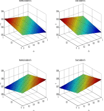
Case 1: In this case the problem was run with =1.14 at = 0.5, we note that >ℎ, there is no

need to run this problem with P.A.D.(i.e = 0), the numerical solution of the standard

Galerkin(G.) finite element method are convergent to the exact solution{see Figure (5.2.1)}.

Figure 5.2.1: a- Numerical solution of G. method of and , b-Exact solution of and ,

at =18, =.5 and =1.14 . 0 0.2 0.4 0.6 0.8 1 0 0.5 1 0.61 0.62 0.63 0.64

a -Numerical solution of u

uh 0 0.2 0.4 0.6 0.8 1 0 0.5 1 0.61 0.62 0.63 0.64

b -Exact solution of u

u 0 0.2 0.4 0.6 0.8 1 0 0.5 1 0.86 0.87 0.88 0.89

a -Numerical solution of v

vh 0 0.2 0.4 0.6 0.8 1 0 0.5 1 0.86 0.87 0.88 0.89

b -Exact solution of v

(21)

21

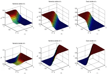
Case 2: In this case we take = and = respectively at = 0.5, we note that <ℎ, thus

we expect to see instability for standard G. finite element method, in Figure{(5.2.2)(a) and

(5.2.3)(a)}the problem run without P.A.D.(i.e. = 0), we see that the standard G. finite

element method produce an oscillating solution which is not close to the exact solution

especially when decreasing with respect to ℎ. In Figure{(5.2.2)(b) and (5.2.3)(b) the problem

run with G.P.A.D. finite element method. where, = 0.25∗ ℎ, where the numerical solution

became more convergent to the exact solution.

Figure 5.2.2 : a- Numerical solution of G. method without P.A.D. of and ,

b- Numerical solution of G.P.A.D. of and , c- Exact solution of and , at =18, =.5 and = .

0 0.5 1 0 0.5 1 0.4 0.6 0.8

uh 0 0.5 1 0 0.5 1 0.5 1 1.5

vh 0 0.5 1 0 0.5 1 0.5 0.6 0.7 0.8 0.9

b -Numerical solution of u

uh 0 0.5 1 0 0.5 1 0.5 0.6 0.7 0.8 0.9

c -Exact solution of u

u 0 0.5 1 0 0.5 1 0.7 0.8 0.9 1

c -Exact solution of v

v 0 0.5 1 0 0.5 1 0.7 0.8 0.9 1

b -Numerical solution of v

(22)

22

Figure 5.2.3 : a- Numerical solution of G. method without P.A.D. of and ,

b- Numerical solution of G.P.A.D. of and , c- Exact solution of and , at =18, =.5 and = .

6 - CONCLUSIONS

From the theoretical analysis and the numerical results ,we can conclude the following :

1-The continuity and V-elliptic of ( , ) and ( , ) is satisfied.

2-The G.P.A.D. finite element method satisfy the stability .

3-Theoretical analysis shows that G.P.A.D. finite element method are convergent with (ℎ ).

4-The G.P.A.D. method removed all oscillations occur when we use the standard Galerkin in the convection-dominated case, and the numerical solutions obtained from this method are consistent with the exact solution.

0 0.5 1 0 0.5 1 0 0.5 1

uh 0 0.5 1 0 0.5 1 0.5 1 1.5

vh 0 0.5 1 0 0.5 1 0.4 0.5 0.6 0.7 0.8

b -Numerical solution of u

uh 0 0.5 1 0 0.5 1 0.5 0.6 0.7 0.8 0.9

c -Exact solution of u

u 0 0.5 1 0 0.5 1 0.7 0.8 0.9 1

c -Exact solution of v

v 0 0.5 1 0 0.5 1 0.7 0.8 0.9 1 1.1

b -Numerical solution of v

(23)

23

REFERENCES

1. Atwell, J. A. and King, B.B., 2000, ''Stabilized finite element methods and feedback control

for Burgers' equation'', Interdisciplinary center for applied Mathematics ,Virginia tech, Blacksburg, VA 24061-0531, Proceedings of the American Control Conference Chicago, Illinois, pp. 2745-2749 .

2. Boules, A. N. , 1998 , "On the existence of the solution of Burgers' equation for n ≤4",

Department of Mathematical Sciences, University of North Florida, Internat. J. Math. & Math. Sci. VOL. 13 NO. 4, pp. 645-650 .

3. Chan, J., Demkowicz, L., Moser, R. and Roberts, N., 2010, ''A New Discontinuous

Petrov-Galerkin Method with Optimal Test Functions. Part V: Solution of 1-D Burgers’ and Navier-Stokes Equations '' , The Institute for Computational Engineering and Sciences, The University of Texas at Austin, Austin, TX 78712, USA.

4. Diez, D. C., Gunzburger, M. and Kunoth, A., 2008, ''An Adaptive Wavelet Viscosity Method

for Hyperbolic Conservation Law'' , Wiley Inter Science, DOI 10.1002/num.20322, pp.1388– 1404.

5. Heitmann ,N.F., 2002,''Subgridscale eddy viscosity for convection dominated diffusive

transport'', Department of Mathematics ,Pittsburgh University.

6. Heitmann, N. F., 2002,"A stabilization scheme for convection dominated diffusive

transport", Department of Mathematics , Pittsburgh University.

7. Kashkool, H. A. and Noon, N. J., 2012, "The Modification of Galerkin and

Galerkin-Conservation Finite Element Methods For Solving Coupled Burgers' Problem", (To appear) in Misan Journal of Academic Studies.

8. Larson, M., G., Bengzon, F., 2013,"The Finite Element Method: Theory, Implementation,

and Applications", Texts in Computational Science and Engineering, ISSN 1611-0994, Verlag Berlin Heidelberg.

9. Srivastava,V. K., Tamsir, M., Bhardwaj, U., Sanyasiraju, Y., 2011, ''Crank Nicolson finite

(24)

24

10. Volkwein, S., 2003, ''Upwind techniques and mixed finite elements for the steady-state

Burgers' equation", Institute of Mathematics, Karl -Franzens-University of Graz, Heinrichstrasse36, A-8010 Graz, Austria.

11. Yang, Q., 2013, "The Upwind Finite Volume Element Method for Two-Dimensional Burgers