Support Vector Hazards Machine: A Counting Process Framework for Learning Risk Scores for Censored Outcomes

(1)

Support Vector Hazards Machine: A Counting Process

Framework for Learning Risk Scores for Censored Outcomes

Yuanjia Wang [email protected]

Department of Biostatistics Mailman School of Public Health Columbia University

New York, NY 10032, USA

Tianle Chen [email protected]

Biogen

300 Binney Street

Cambridge, MA 02142, USA

Donglin Zeng [email protected]

Department of Biostatistics

University of North Carolina at Chapel Hill Chapel Hill, NC 27599, USA

Editor:Karsten Borgwardt

Abstract

Learning risk scores to predict dichotomous or continuous outcomes using machine learning approaches has been studied extensively. However, how to learn risk scores for time-to-event outcomes subject to right censoring has received little attention until recently. Existing approaches rely on inverse probability weighting or rank-based regression, which may be inefficient. In this paper, we develop a new support vector hazards machine (SVHM) approach to predict censored outcomes. Our method is based on predicting the counting process associated with the time-to-event outcomes among subjects at risk via a series of support vector machines. Introducing counting processes to represent time-to-event data leads to a connection between support vector machines in supervised learning and hazards regression in standard survival analysis. To account for different at risk populations at observed event times, a time-varying offset is used in estimating risk scores. The resulting optimization is a convex quadratic programming problem that can easily incorporate non-linearity using kernel trick. We demonstrate an interesting link from the profiled empirical risk function of SVHM to the Cox partial likelihood. We then formally show that SVHM is optimal in discriminating covariate-specific hazard function from population average hazard function, and establish the consistency and learning rate of the predicted risk using the estimated risk scores. Simulation studies show improved prediction accuracy of the event times using SVHM compared to existing machine learning methods and standard conventional approaches. Finally, we analyze two real world biomedical study data where we use clinical markers and neuroimaging biomarkers to predict age-at-onset of a disease, and demonstrate superiority of SVHM in distinguishing high risk versus low risk subjects.

(2)

1. Introduction

Time-to-event outcome is of interest in many scientific studies in which right censoring oc-curs when subjects’ event times are longer than the duration of studies or subjects drop out of the study prematurely. One important goal in these studies is to use baseline covariates collected on a newly recruited subject to construct an effective risk score to predict likeli-hood an event of interest. For example, in one of our motivating studies analyzed in Section 4.2 (PREDICT-HD, Paulsen et al. 2008a), the research aim is to combine neuroimaging biomarkers with clinical markers measured at the baseline to provide risk stratification for time-to-onset of Huntington’s disease (HD) to facilitate early diagnosis, where subjects who did not experience HD during the study had censored HD onset time. This critical goal of identifying prognostic markers predictive of disease onset is shared by research commu-nities on other neurological disorders such as Alzheimer’s disease and Parkinson’s disease, and recognized as one of the primary aims in research initiatives such as Alzheimer’s Dis-ease Neuroimaging Initiative (Mueller et al., 2005) and Parkinson’s Progression Markers Initiative (Marek et al., 2011).

Learning risk scores for binary or continuous outcomes are examined extensively in sta-tistical learning literature (Hastie et al., 2009). However, learning risk scores for occurrence of an event subject to censoring is much less explored. Existing work on survival analysis focuses on estimating population-level quantities such as survival function or association parameters through hazard function. For example, the most popular model for the time-to-event analysis is the Cox proportional hazards model (Cox, 1972), which assumes the hazard ratio between two subjects with different covariate values stays as a constant as time progresses. A Cox partial likelihood function is maximized for estimation. When the pro-portional hazards assumption is violated, several alternative models have been proposed in statistics literature, including the proportional odds model (Bennett, 1983), the accelerated failure time model (Buckley and James, 1979), the linear transformation models (Dabrowska and Doksum, 1988; Cheng et al., 1995; Chen et al., 2002), and more recently general transfor-mation models (Zeng and Lin, 2006, 2007). The above models are all likelihood-based which impose certain parametric or semiparametric relationship between the underlying hazard function and the covariates. In addition, they are designed to estimate the population-level parameters for the association between covariates and the time-to-event outcomes (and thus uses likelihood as the optimization function), but do not directly focus on individual risk scores for predicting an event time.

(3)

geometric interpretation. In addition, the algorithm can be written as a strictly convex op-timization problem, which leads to a unique global optimum and incorporates non-linearity in an automatic manner using various kernel machines. By reformulating the algorithm into a minimization of regularized empirical risk, Steinwart (2002) established the univer-sal consistency and learning rate on some functional space. Support vector machines have also been applied to continuous outcomes through regression (Smola and Sch¨olkopf, 2004), multicategory discrete outcomes (Lee et al., 2004), and structured classification problems (Wang et al., 2011).

For time-to-event outcomes, right censoring makes developing supervised learning tech-niques challenging due to missing event times for censored subjects and a lack of standard prediction loss function. Ripley and Ripley (2001) and Ripley et al. (2004) discussed models for survival analysis based on neural network. Bou-Hamad et al. (2011) reviewed survival tree approaches in the recent work as non-parametric alternatives to semiparametric mod-els. Compared to survival trees, effectively extending the support vector–based methods to censored data is still an on-going research. Shivaswamy et al. (2007) and Khan and Zubek (2008) proposed asymmetric modifications to the -insensitive loss function of sup-port vector regression (SVR) to handle censoring. Specifically, they penalized the censored and non-censored subjects using different loss functions to extract incomplete information due to censoring. Van Belle et al. (2010) proposed a least-squares support vector machine, where they adopted the concept of concordance index and added rank constraints to handle censored data. In their method, the empirical risk of miss-ranking two data points with respect to their event times was minimized. Furthermore, Van Belle et al. (2011) conducted numerical experiments to compare some recent machine learning methods for censored data and proposed a modified procedure to adjust for censoring based on both rank and regres-sion constraints. Their results indicate that including two types of constraints performs the best regarding the prediction accuracy. None of the above methods has theoretical justification and the relationship between their objective loss functions to be minimized and the goal of predicting survival time remains unclear. The rank-based methods only use feasible pairs of observations whose ranks are comparable so that it may result in potential selection bias when constructing prediction rules, especially when the censoring mecha-nism is not completely at random (e.g., censoring time depends/correlates with a subject’s covariates). Recently, Goldberg and Kosorok (2013) used inverse-probability-of-censoring weighting to adapt standard support vector methods for complete data to censored data. However, inverse weighting is known to be inefficient (Robins et al., 1995) due to the fact that it discards useful information for some subjects known to survive longer than observed times, and in addition, this method may exhibit severe bias when the censoring distribution is misspecified. Additionally, the weights used in the inverse weighting can be large in some situations, and computation of Goldberg and Kosorok (2013) becomes numerically unstable and even infeasible.

(4)

if a prediction rule can adequately predict the event time, the same rule should also predict the counting process at any given time that a subject is still at risk. We propose a flexible nonparametric decision function with an additive structure for the counting process, which gives the desirable risk scores but also includes a time-varying offset to account for different at-risk population as time progresses. Empirically, we transform the prediction of an event time to predicting a sequence of binary outcomes for which algorithm such as support vector machine (SVM) is standard and commonly used. This transformation allows for the success-ful statistical learning tools designed for classification and prediction of binary outcomes to be used for censored outcomes without modeling the censoring distribution. The developed algorithm formulation is similar to the standard support vector machines and can be solved conveniently using any convex quadratic programming packages. In addition, theoretical analysis shows that the optimal rule obtained from SVHM is equivalent to maximizing the difference between the instantaneous subject-specific hazards and population-average hazard, which intuitively links SVHM to the commonly used hazards regression models in traditional survival analysis. The profile loss shares similarity with Cox partial likelihood. Under some regularity conditions, we show the universal consistency of SVHM and derive corresponding finite sample bounds on the deviation from the optimal risk. Numeric simu-lations and applications to real world studies show superior performance in distinguishing high risk versus low risk subjects.

2. Learning Risk Scores with SVHM

In this section, we first introduce the population loss function that SVHM aims to optimize with infinite sample and its corresponding Bayes risk. Next, we lay out the algorithm to empirically learn the risk scores and assess the empirical risk.

2.1 Review of Survival Analysis and Introduction of Counting Process Framework for SVHM

We begin by briefly introducing basic concepts and notation of classical survival analysis (c.f. Fleming and Harrington, 1991). Survival analysis focuses on using covariates to predict time to event outcomes. The events of interest can be death, diagnosis of a disease, onset of cancer metastasis, or failure of a machine component. An event time of interest (i.e., age at onset of a disease) is usually denoted byT, and a vector of baseline covariates (e.g., genomic risk factors) is denoted byX. The main goals of survival analysis are to understand association between X and T or predicting T fromX. A fundamental problem of survival analysis is to deal with incomplete observation ofT due to that the event may not occur in some of the subjects due to study termination or subjects dropping out of the study. For example, in a study on predicting time to cancer metastasis, some subjects may not develop metastasis by the end of study period, and thus theirT is not observed. These subjects are termed as being censored and their time to study termination is termed as censoring time, usually denoted byC. For each subject in the study, we observe either their event time T

or censoring time C, whichever is smaller. This observation is usually denoted by Ti∧Ci,

(5)

for i = 1, . . . , n, where I(·) is an indicator function and I(Ti ≤ Ci) is thus the event

indicator. The central quantity of interest in a survival analysis is occurrence of an event over time. Such occurrences are equivalent to point processes described by counting the number of events as they occur by certain time point, termed as counting processes. That is, a counting process of the event on subjecticounts the number of events that have occurred up to, and including t, and is denoted as Ni(t) = I[(Ti ∧Ci) ≤ t]. Corresponding to the

counting process for the events, the at-risk process counts subjects who have not yet had an event by time tand thus who are still “at risk” of experiencing an event. Such process is denoted byYi(t) =I[(Ti∧Ci)≥t].

The fundamental idea to learn risk scores for T to distinguish high risk versus low risk subjects is to equivalently learn risk scores for the counting process associated with T at each time point. Since the latter can be treated as a sequence of binary outcomes (event vs. no event) over time, it motivates one to reformulate the problem as deriving the risk score for predicting the jumps of the counting process over a sequence of time points among subjects still at risk at those times. This amounts to developing a classification rule to predict whether a subject will experience an event in the next immediate time point given that the subject has not yet experienced an event. To account for different risk sets as time progresses (i.e., risk set at timetis the subset of subjects withYi(t) = 1) , it is necessary to

include a time-varying offset for the nonparametric risk score. Thus, consider the following general form at timet for a subject with X=x,

f(t,x) =α(t) +g(x), (1) where both α(·) and g(·) are unknown nonparametric functions, g(x) is the risk score, and

α(t) is the time-varying offset. To understand (1), consider a risk score function at timet

for a subject with X = x: if this subject is still at risk at time t, we predict the subject to experience the event at the next immediate time point if f(t,x) > 0, and predict as event-free if f(t,x) ≤0. Thus, within a small time interval [t, t+dt), where dt denotes a positive infinitesimal unit, a natural prediction loss counting rate of risk-misclassification is given by

Y(t)dN(t)I(f(t,X)<0) +Y(t)(1−dN(t))I(f(t,X)≥0),

where Y(t) and X are the at risk process and covariates for a subject drawn from the population, respectively, and dN(t) denotes the number of jumps of the counting process

N(t) in a small time interval [t, t+dt). Equivalently, dN(t) = 1 if T ∈ [t, t+dt) and

dN(t) = 0 otherwise, so it is a binary variable taking value one if an event occurs in the interval [t, t+dt) for subjects who are still at risk for experiencing an event. Thus, summing above loss function over subjects counts the number of at-risk subjects miss-classified by the prediction rulef(t,X). The above prediction loss can be viewed as a natural extension of the 0-1 loss for binary case to capture the same information for an at-risk subject in a survival analysis: if the prediction function and the observed counting process at time t

(6)

weighted loss, where the ratio of weights for two unbalanced classes is proportional to

E[dN(t)]/E[Y(t)]:

Y(t)dN(t)I(f(t,X)≤0) +E[dN(t)]

E[Y(t)] Y(t)(1−dN(t))I(f(t,X)≥0). (2) This weighting scheme can also be understood in the context of nested case-control design. That is, select one subject from the event class,{i:dNi(t) = 1}, at this interval and another

subject from the non-event class,{i:dNi(t) = 0}, using E[dN(t)]/E[Y(t)] as the sampling

weights for the latter. Consequently, an overall weighted prediction loss for the proposed SVHM, which is the expectation of (2) and ignores infinitesimal terms, is

R0(f) =E Z

Y(t)I[f(t,X)≤0]dN(t)

+

Z

E(Y(t)I[f(t,X)≥0])

E(Y(t)) E(dN(t)),

where the expectation is with respect to random variables Y(t) and dN(t). Our goal of learning a prediction rule for T, or equivalently, N(t), based on the censored data is to minimize the population loss R0(f).

To define the empirical loss, suppose there aremdistinct ordered event times,t1< t2< . . . < tm. We let

δNi(tj)≡2(Ni(tj)−Ni(tj−))−1

soδNi(tj) takes values 1 or−1 depending on whether theith subject experiences an event

at tj or not. Learning f(t,x) becomes a sequence of binary classification problems over tj’s. Furthermore, at each tj and for subject i at risk at tj, we use the following weight

associated with the risk set size attj:

wi(tj) =I{δNi(tj) = 1}

1−_Pn 1

i=1Yi(tj)

+I{δNi(tj) =−1}

1

Pn

i=1Yi(tj)

.

Note that the weightswi(tj) are the empirical version of the weights used in (2) with similar

interpretation as the reciprocal of the empirical probability of remaining event free or expe-riencing an event at the observed event time. Such weights balance the differential size of event class and non-event class at timetj. Then an optimal decision function that minimizes

the empirical version ofR0(f) is to minimize the following weighted total misclassification

error:

R0n(f) =n−1 n X

i=1 m X

j=1

wi(tj)Yi(tj)I(δNi(tj)f(tj,Xi)<0), (3)

where the termYi(tj) reflects that only subjects still at risk will contribute towards

predic-tion.

Directly minimizing (3) is difficult due to non-smoothness of the 0-1 loss in the indicator function. Furthermore, no restriction on the complexity of f leads to potential overfitting. To handle these issues, we adopt the same idea as SVM for supervised learning to replace the 0-1 loss in (1) by the hinge loss, and impose regularization to estimatef. Specifically, we propose to minimize the following regularized SVHM loss:

(7)

with R_n(f)≡n−1 n X

i=1 m X

j=1

wi(tj)Yi(tj)[1−f(tj,Xi)δNi(tj)]+, (4)

where [1−x]+ = max(1−x,0) is the hinge loss, k · k is a suitable norm or semi-norm for f to be discussed in the following sections, and λn is the regularization parameter. This

minimization is equivalent to maximizing the margin between subjects in the event and non-event classes subject to an upper bound on the misclassification rate. Since this learning method is a weighted version of the standard support vector machines and learningf(t,x) is essentially learning the hazard rate function, we refer our proposed method as “support vector hazards machine”.

2.2 Learning Algorithm

Next, we describe the computational algorithm to solve the optimization in (4). We do not impose any restriction on α(t), and assumeg(x) lies in a reproducing kernel Hilbert space

Hn with a kernel function K(x,x0). Commonly used kernels include linear kernel, where K(x,x0) =hx,x0i; radial basis kernel, whereK(x,x0) = exp(−kx−x0k2_/σ_{); and}_l_th-degree

polynomial kernel, whereK(x,x0) = (1 +hx,x0i)l. Furthermore, let kfk=kgkHn which is the norm in the reproducing kernel Hilbert spaceHn. The minimization in (3),

min

α,g

1

n n X

i=1 m X

j=1

wi(tj)Yi(tj)[1−(α(tj) +g(Xi))δNi(tj)]++λnkgk2Hn, (5)

is equivalent to

min

α,g

1 2kgk

2

Hn+Cn

n X

i=1 m X

j=1

wi(tj)Yi(tj)ζi(tj), (6)

subject to Yi(tj)ζi(tj)≥0, i= 1,· · ·, n, j = 1,· · · , m,

Yi(tj)δNi(tj){α(tj) +g(Xi)} ≥Yi(tj){1−ζi(tj)}, i= 1,· · · , n, j = 1,· · · , m,

where the valueζi(tj) is the proportional amount by which the prediction is on the wrong

side of its margin at timetj, andCn is the cost parameter.

The constrained optimization in (6) is usually solved by turning it into its dual form (through including Lagrange multipliers of the constraints into the objective function). We convert the above problem to its dual form by using the corresponding Lagrangian function

Lp =

1 2kgk

2

Hn+Cn

n X

i=1 m X

j=1

wi(tj)Yi(tj)ζi(tj)− n X

i=1 m X

j=1

µijYi(tj)ζi(tj)

−

n X

i=1 m X

j=1

γij[Yi(tj)δNi(tj){α(tj) +g(Xi)} −Yi(tj){1−ζi(tj)}],

where µij ≥0 and γij ≥0 are the corresponding Lagrange multipliers. Let{φ1, φ2, ...} be

(8)

the Lagrangian function with respect toβ’s,α(tj)’s andζi(tj)’s, we obtain

βk= n X i=1 m X j=1

γijYi(tj)δNi(tj)φk(Xi), k= 1,2,· · · ,

n X

i=1

γijYi(tj)δNi(tj) = 0,

Cnwi(tj)Yi(tj)−µijYi(tj) =γijYi(tj), i= 1,· · ·, n, j= 1,· · ·, m,

as well as the positivity constraints γij, µij, ζi(tj) ≥ 0 for all i and j. By substituting

these back toLp and noting thatP∞_k₌₁φk(Xi)φk(X) =K(Xi,X) (Theorem 4.2, Steinwart

(2002)), we obtain the dual objective function to be

LD = n X i=1 m X j=1

γijYi(tj)−

1 2 n X i=1 n X

i0₌₁

m X

j=1 m X

j0₌₁

γijγi0_j0Y_i(t_j)Y_i0(t_j0)δN_i(t_j)δN_i0(t_j0)K(X_i,X_i0),

(7) and the optimization is carried out by maximizing LD with respective to γij subject to

0 ≤ γij ≤ wi(tj)Cn and Pn_i₌₁γijYi(tj)δNi(tj) = 0 for i = 1, . . . , n and j = 1, . . . , m.

This optimization can be solved using quadratic programming packages available in many softwares (for example, MOSEK toolbox in Matlab). The tuning parameter Cn is chosen

by cross-validation searching over a grid of values. Denote _bγij as the solutions for γij

obtained from the optimization procedure in (7). Comparing (7) with existing standard support vector machine algorithms, we see that the objective function sums across all at-risk subjects and across all time points for which they are at at-risk. Constraints are placed on those subjects and time points.

Next, from the equalities between βk’s and γij’s in the above duality derivation, the

solutions forβk (denoted asβb_k) are given by

b βk=

n X i=1 m X j=1 b

γijYi(tj)δNi(tj)φk(Xi), k= 1,2,· · · .

Thus, the solution forgthat minimzies (5), which is the risk score for a future subject with baseline covariates x, is

b g(x) =

∞ X

k=1 b

βkφk(x) = n X i=1 m X j=1 b

γijYi(tj)δNi(tj) ∞ X

k=1

φk(Xi)φk(x)

= n X i=1 m X j=1 b

γijδNi(tj)K(x,Xi).

It follows that those data points withγbij >0 form support vectors and determineg(X).

Furthermore, to determine the solution to α(tj) at each tj, denoted by αb(tj), we solve

the Karush-Kuhn-Tucker (KKT) conditions

(9)

Yi(tj)ζi(tj)≥0,

Yi(tj)δNi(tj){α(tj) +g(Xi)} −Yi(tj){1−ζi(tj)} ≥0.

Specifically, if there are some support vectors lying on the edge of the margin which are characterized by 0 < bγij < wi(tj)Cn, αb(tj) = 1/δNi(tj)−bg(Xi) for these points, and we

take the average of all the solutions for numerical stability. If all the support vectors at tj

are_bγij =Cnwi(tj), ˆα(tj) is not unique and falls into a range

min

Yi(tj)=1,ˆγij=Cnwi(tj),

δNi(tj)=1

{1−_bg(Xi)} ≥αˆ(tj)≥ max

Yi(tj)=1,γˆij=Cnwi(tj),

δNi(tj)=−1

{−1−_bg(Xi)}.

In this case, we takeα_b(tj) = 1−bg(Xi) whereδNi(tj) = 1 for some iwithYi(tj) = 1.

Since a higher value of the prediction function αb(t) +bg(x) leads to a greater likelihood

of having an event at an earlier time, the magnitude of _bg(x) induces a natural ordering of the risks. Lastly, the learned risk scores can be used to predict the event time for any future subjects using their baseline covariatesx. To this end, consider the nearest-neighbor prediction: for a future subject with X = x, find k (k=1 or 3 in our applications) non-censored subjects in the training data whose predictive scores are closest to _bg(x), denoted as bg(Xj). To maintain the monotone relationship between the event times and predictive

scores, sort these scores of non-censored subjects in the training data in descending order and identify the rank of _bg(Xj). Next, sort the event times of the derived scores in the

training data in ascending order and find the event times with the same rank as the rank of_bg(Xj), denoted asTj0. The event time for this subject is predicted asT_j0 (or the average

of Tj0 fork= 3). We provide a detailed description of SVHM algorithm in Appendix A.

2.3 Connection with Existing Support Vector-Based Approaches

Support vector-based approaches in machine learning literature are motivated by the fact that they are easy to compute and enable estimation under weak or no assumptions on the distribution. Most of these approaches (Shivaswamy et al., 2007; Van Belle et al., 2010, 2011) adapt the-insensitive loss for SVR to account for incomplete observations in time-to-event data. To improve performance, modified SVR (Van Belle et al., 2011) further places ranking constraints under the -insensitive loss. The formulation of the problem is

min

w,,ξ,ξ∗

1 2w

T_w₊_λ 1

X

i

i+λ2 X

i

(ξi+ξ∗i), (8)

subject towT(ϕ(Xi)−ϕ(Xj(i))≥Yi−Yj(i)−i, i= 1,· · · , n, wTϕ(Xi) +b≥Yi−ξi, i= 1,· · · , n,

∆i(wTϕ(Xi) +b)≥ −∆iYi−ξi∗, i= 1,· · ·, n, i≥0, ξi ≥0, ξ∗i ≥0, i= 1,· · ·, n,

whereYi =Ti∧Ci,ϕ(·) is the feature map that does not need to be specified explicitly in a

kernel-based method, andj(i) indicates the subject with the largest event time smaller than

Zi. The first set of constraints above aims at ensuring rank consistency to maximize

(10)

same as the regression constraints in Shivaswamy et al. (2007) for the modified-insensitive loss for survival outcomes. One potential problem with the above optimization is that the observations contributing to these three sets of constraints may consist of a selected (non-censored) sample from the full data; thus, the derived prediction rule will likely favor those observations which contribute most.

Furthermore, comparing the modified SVR in (8) with SVHM in (6), we see that the loss function for the former is the -insensitivity loss plus the loss resulting from violating rank consistency, while for the latter it is sum of a sequence of hinge losses. The objective function and the slack variables (i.e., i, ξi, ξi∗) for the modified SVR, however, are

time-invariant, while the slack variables for SVHM (i.e., ζi(tj) in (8)) are time-sensitive. Thus,

we expect better control of the prediction error by SVHM. Note that this advantage stems from the counting process formulation of SVHM transforming prediction of time-to-event outcomes (or survival outcomes) as a sequence of binary prediction problems over time.

2.4 Connection with the Cox Partial Likelihood

In classical survival analysis using Cox regression model (Cox, 1972), partial likelihood plays a central role since it only involves association parameter of interest (i.e., hazard ratios as regression coefficients) but not the nuisance parameter (i.e., baseline hazard function), and maximizing the partial likelihood directly estimates the hazard ratios. The partial likelihood is constructed by multiplying together the conditional probabilities of observing an event for individualiat time t, given the past and given that an event is observed at that time, over all observed event times. This conditional probability formulation shares some similarity with our hazard formulation for SVHM. Since maximizing Cox partial likelihood leads to regression estimators that enjoy optimal statistical property (i.e., being semiparametric efficient, Bickel et al. (1998)), it is worth to draw connection between SVHM and partial likelihood to shed lights on the theoretical properties of SVHM.

To this end, we further explore the optimization in (5) to compare the SVHM objective function and the Cox partial likelihood. First note that the functionα(t) in (5) is analogous to the baseline hazard function in the Cox model (Cox, 1972), which is treated as a nuisance parameter and profiled out for inference. Thus, we also profile out α(t) to investigate the profile risk function for SVHM (e.g., substitute fitted α(t) in the original risk function). For a fixed g(x), from the derivation similar to Hastie et al. (2009) (p421) and Abe (2010) (p77), we can show that at each tj, if there are some support vectors lying on the edge of

the margin which are characterized by 0< γij < wi(tj)Cn, these margin points can be used

to solve forα(tj). This yields

b

α(tj) = 1−g(Xi), δNi(tj) = 1.

Note thatXi is the covariate value for the subject who has an event at tj. However, if γij

is not within (0, wi(tj)Cn,αb(tj) can be any value satisfying

min

b

γij=Cnwi(tj),

δNi(tj)=1

{1−g(Xi)} ≥α(tj)≥ max b

γij=Cnwi(tj),

δNi(tj)=−1

(11)

In this case, takingα_b(tj) = 1−g(Xi) where δNi(tj) = 1 satisfies these constraints. Further

note that optimizing (5) is equivalent to minimizing

1 n n X i=1 d X j=1

Yi(tj)wi(tj)[1−(α(t) +g(Xi))δNi(tj)]++λnkgkHn

= 1 n n X i=1 Z

[1−(α(t) +g(Xi))]+dNi(t) +

1

n

Z Pn

i=1Yi(t)[1 + (α(t) +g(Xi))]+ Pn

i=1Yi(t)

d

( _n

X

i=1 Ni(t)

) −1 n n X i=1 Z ₁ Pn i=1Yi(t)

([1−(α(t) +g(Xi))]++ [1 + (α(t) +g(Xi))]+)dNi(t) +λnkgkHn.

After we plug the expression of α_b(t) = Pn

i=1(1−g(Xi))I(δNi(t) = 1) into the above

expression, we obtain

1 n n X i=1 Z

[1−(α_b(t) +g(Xi))]+dNi(t) =

1

n n X

i=1

∆i[1−(1−g(Xi) +g(Xi))])+ = 0,

and similarly, 1 n n X i=1 Z 1 Pn i=1Yi(t)

([1−(αb(t) +g(Xi))]++ [1 + (αb(t) +g(Xi))]+)dNi(t) =

2 n n X i=1 Z

dNi(t) Pn

i=1Yi(t) .

Additionally,

1

n

Z Pn

i=1Yi(t)[1 + (αb(t) +g(Xi))]+ Pn

i=1Yi(t)

d

( _n

X

i=1 Ni(t)

) = 1 n n X k=1 ∆k Pn

i=1I(Yi ≥Yk)[1 + (αb(Xk) +g(Xj))]+ Pn

i=1I(Yi ≥Yk)

= 1 n n X k=1 Pn

i=1I(Yi≥Yk)[2−g(Xk) +g(Xi)]+ Pn

i=1I(Yi≥Yk)

∆k.

The objective function (5) can be written asPR_n(g) +λnkgk2Hn,where

PR_n(g) = 1

n n X

i=1

Z Pn

k=1Yk(t)[2−g(Xi) +g(Xk)]+ Pn

k=1Yk(t)

dNi(t)−

2 n n X i=1 Z _dN

i(t) Pn

k=1Yk(t)

= 1 n n X i=1 ∆i Pn

k=1I(Yk≥Yi)[2−g(Xi) +g(Xk)]+ Pn

k=1I(Yk≥Yi)

− 2 n n X i=1 ∆i Pn

k=1I(Yk≥Yi)

= Pn ∆

e

Pn{I(Ye ≥Y)[2 +g(Xe)−g(X)]₊} e

Pn[I(Ye ≥Y)]

!

− 2 nPn

(

∆

e

Pn[I(Ye ≥Y)] )

.

Here,Pndenotes the empirical measure fromnobservations andPe_nis the empirical measure

(12)

If we let fb(x, t) = α_b(t) +_bg(x) be the function minimizing (5) overg ∈ H_n, then R_n(fb) =

PRn(gb).

In a Cox partial likelihood function, g(X) is estimated by minimizing

Pn ∆ log e

Pn{I(Ye ≥Y) exp{g(Xe)−g(X)}} e

Pn[I(Ye ≥Y)]

! .

Therefore, it is worthy to point out one interesting observation: bothPR_n(g) and the Cox partial likelihood take a similar form which essentially evaluates a loss comparing the risk scores from the subjects at risk versus the one from the subject who has an event at the same time. SVHM uses a hinge loss while Cox partial likelihood uses an exponential loss and a logarithm transformation, which is similar to the contrast between SVM and logistic regression. The robustness of hinge loss compared to exponential loss suggests SVHM will be less sensitive to extreme observations. In addition, this connection sheds lights on the theoretical optimality of SVHM which we prove in the next section.

3. Theoretical Properties

In this section, we study the asymptotic properties of SVHM and the predicted risk. We first derive the population risk function for the proposed SVHM. Next, we derive the optimal fully nonparametric decision rule for this risk function and show that it also optimizes the 0-1 loss corresponding to (3). We highlight important differences in the theoretical proof that distinguish this work from the standard proofs in the statistical learning theories.

3.1 Risk Function and Optimal Risk Classification Rule

To derive the population risk function for SVHM, we first examine the population version (the expectation) of R_n(f). Recall the definition ofR_n(f) is given in (4) as

Rn(f) =n−1 n X

i=1 m X

j=1

I{δNi(tj) = 1}(Pnl=1Yl(tj)−1) Pn

l=1Yl(tj)

[1−f(tj,Xi)]+

+n−1 n X

i=1 m X

j=1

I{δNi(tj) = 1} Pn

l=1Yl(tj)

[1 +f(tj,Xi)]+.

After re-arranging the terms and adopting counting process notation, we can rewriteR_n(f) as

Rn(f) =

1

n n X

i=1 Z

Yi(t)[1−f(t,Xi)]+dNi(t) +

1

n

Z Pn

i=1Yi(t)[1 +f(t,Xi)]+ Pn

i=1Yi(t)

d

( _n

X

i=1 Ni(t)

)

−1 n

n X

i=1

Z ₁

Pn i=1Yi(t)

([1−f(t,Xi)]++ [1 +f(t,Xi)]+)dNi(t).

Note that the last term in Rn(f) is on the order of O(1/n), so it vanishes as n goes to

(13)

R(f), to be

R(f) =E Z

Y(t)[1−f(t,X)]+dN(t)

+

Z _E₍_Y₍_t_{)[1 +}_f₍_t,_X_)] +)

E(Y(t)) E(dN(t)).

Likewise, similar arguements show that the empirical risk based on the prediction error in (1), i.e., R₀_n(f), converges toR₀(f).

Let f∗(t,x) denote the limit of the risk function estimated by SVHM (i.e., the optimal function minimizing R(f)). Since the difference between R(f) and R₀(f) is the hinge loss versus the zero-one loss, one question is whether f∗(t,x) also minimizes R₀(f). The following theorem gives such a result forf∗(t,x).

Theorem 3.1 Leth(t,x) denote the conditional hazard rate function ofT =tgivenX=x

and let ¯h(t) = E[dN(t)/dt]/E[Y(t)] = E[h(t,X)|Y(t) = 1] be the average hazard rate at time t. Then f∗(t,x) = sign(h(t,x)−¯h(t)) minimizes R(f). Furthermore, f∗(t,x) also

minimizes R0(f) and

R0(f∗) =P(T ≤C)−

1 2E

Z

E(Y(t)|X=x)|h(t,x)−¯h(t)|dt

.

In addition, for any f(t,x)∈[−1,1],

R₀(f)− R₀(f∗)≤ R(f)− R(f∗),

where h(t,x) denotes the conditional hazard rate of T = t given X = x and ¯h(t) is the

population average hazard at time t,

¯

h(t) = E[dN(t)]/dt

E[Y(t)] =E[h(t,X)|Y(t) = 1].

The proof of Theorem 3.1 is provided in the Appendix B. Theorem 3.1 resembles the excess risk in most learning theories (Bartlett et al., 2006); however, the loss function in our case is some composite expectation, R0(f), which is not covered by Bartlett et al.

(2006). From Theorem 3.1, we see that the optimal rule is essentially to predict whether an at-risk subject will experience an event by comparing the subject-specific hazard rate depending on the covariate to the population-average hazard rate obtained from all at-risk subjects at a given time point. Since the minimizer of R(f) also minimizes R₀(f), this theory justifies the use of hinge-loss in SVHM to minimize the weighted prediction error inR0(f). The last inequality in Theorem 3.1 proves that a decision function with a small

excess hinge-loss–based risk will lead to a small excess 0-1 loss–based risk.

3.2 Asymptotic Properties

Here, we study the asymptotic properties of SVHM when the decision function takes the form in (1). Specifically, we examine a stochastic bound for the excess risk when using _bg, the estimator from n observations. This bound will be given in terms of the sample size

(14)

a reproducing kernel Hilbert space from a Gaussian kernelk(x, x0) = exp{−kx−x0k2_/σ n}.

Instead of considering the risk for R(f), we consider

PR(g) = min

α(t)

R(α(t) +g(x))

and refer it as “profile risk”, since α(t) is profiled out from the original risk function. In other words, PR(g) is the best expected risk for a given score g(x) after accounting for

α(t).

To obtain an explicit expression of PR(g), we first note that

R(α(t) +g(x)) = E Z

Y(t)[1−f(t,X)]+dN(t)

+

Z _E₍_Y₍_t_{)[1 +}_f₍_t,_X_)] +)

E(Y(t)) E(dN(t))

=

Z

E[Y(t)h(t,X)]

E[Y(t)h(t,X)]−E[Y(t)g(X)h(t,X)]

E[Y(t)h(t,X)] −α(t)

+ dt

+

Z

¯

h(t)E[Y(t)]

E[Y(t)] +E[Y(t)g(X)]

E[Y(t)] +α(t)

+ dt.

Sinceα(t) is arbitrary and the integrand in the above expression is a piecewise linear function of α(t), simple algebra gives that

α(t) =−E[Y(t)] +E[Y(t)g(X)] E[Y(t)]

minimizes R(f). Therefore, after replacing α(t) by this minimizer in R(α(t) +g(x)), we obtain

PR(g) =E "

∆PIe ( ˜Y ≥Y)[2−g(Xe) +g(X)]+

e

PI( ˜Y ≥Y)

#

.

Clearly,PR(g) is the asymptotic limit ofPRn(g). The following theorem holds for the risk

PR(bg).

Theorem 3.2 Assume that X’s support is compact and E[Y(τ)|X] is bounded from zero

where τ is the study duration. Furthermore, assume λn and σn satisfies λn, σn → 0, and

nλnσ(2/p −1/2)d

n → ∞ for some p∈(0,2). Then it holds

λnkbgk 2

Hn+PR(bg)≤inf_g PR(g) +Op (

λn+σnd/2+

λ−1n /2σ−(1n /p−1/4)d

√ n

) .

(15)

kernel and regularization parameter should converge to zero in certain rates depending on

X’s dimension, but not too fast to ensure stochastic variability is under control. Finally, we state two useful observations as remarks below.

Remark 1. From Theorem 3.2, if we choose σn= (nλn)−1/[2d(1/p+1/4)], it gives

PR(bg)− PR(g ∗

) =Op

λn+ (nλn)−q ,

whereq = 1/(4/p+ 1) andg∗ is the function minimizingPR(g).

Remark 2. Furthermore, if we chooseλn=n−q/(q+1), then the optimal rate obtained from

Theorem 3.2 becomes

PR(_bg)− PR(g∗) =O(n−q/(q+1)). 4. Numeric Examples

In this section, we first present simulation results comparing SVHM to existing machine learning approaches and semiparametric approaches based on the Cox proportional hazards regression. Next, we provide applications to two real world empirical studies.

4.1 Simulation Studies

In all scenarios, we generated both event times and censoring times to be dependent on the covariates. First we simulated five covariatesZ= (Z1, . . . , Z5) which are marginally normal N(0,0.52) with pairwise correlation corr(Zj, Zk) =ρ|j−k|, andρ= 0.5. The event times were

generated from the Cox proportional hazards model with trueβ= (2,−1.6,1.2,−0.8,0.4)T and the exponential distribution with λ = 0.25 was assumed to compute the baseline cu-mulative hazard function Λ(t) = R₀tλ0(s)ds, where λ0(s) is the baseline hazard function. We simulated two types of censoring distributions. In the first type, the censoring times were generated from an accelerated failure time model following the log-normal distribution, that is, logC ∼N(ZTβ_c+a,0.52), with true β_c = (1,1,1,1,1)T. In the second type, the distribution of the censoring times follows the Cox proportional hazards model with true

β_c= (1,1,1,−2,−2)T and the baseline cumulative hazard function Λc(t) =bt(b >0). The

parameters a and b were chosen to obtain the desired censoring ratio. We considered the censoring ratios 40% and 60%. Any event times or censoring times greater than u0 were truncated at u0, whereu0 is the 90th percentile of the event times. Moreover, we explored

some generalizations of the above scenarios to include more covariates in the regression models and include additional noise variables. Besides these training data sets (with a sam-ple size of 100 or 200), we use a randomly generated testing data set with 10,000 subjects in each scenario with no censoring to evaluate prediction performance of various methods. For all scenarios, we compared SVHM with the modified support vector regression for right censored data based on the ranking constraints (modified SVR) (Van Belle et al., 2011) and the inverse-probability-of-censoring weighting with censoring distribution estimated using Kaplan-Meier (IPCW-KM) or estimated under a Cox model (IPCW-Cox) (Goldberg and Kosorok, 2013), whose objective function is defined as

n−1 n X

i=1

∆i

b S(Yi)

(16)

withSb(t) is the estimated survival probability for the censoring time. We used linear kernel K(x, x0) =xTx0 in all four methods, and used 5-fold cross-validation to choose the tuning parameters from the grid of{2−16,2−15, . . . ,215,216}. As the model comparison criterion, we adapted mean squared error to censored data, which sums up the mean squared differences between the fitted event times and observed event times for uncensored subjects. For censored subjects, we sum up the squared differences between fitted times and censoring times if the former is smaller than the latter. Essentially, for these censored subjects, if their predicted event times were less than the observed censoring times, we imposed a penalty to measure how much under-estimation there is. The mean squared differences were assumed to be zero for censored subjects if their predicted values were greater than the observed censoring times. We divided the total sum of squares by the total number of observations. We repeated the simulation 500 times, since our results show that 500 repetitions are sufficient to obtain stable simulation results to draw conclusions on comparing performance of different methods while still achieving computational efficiency.

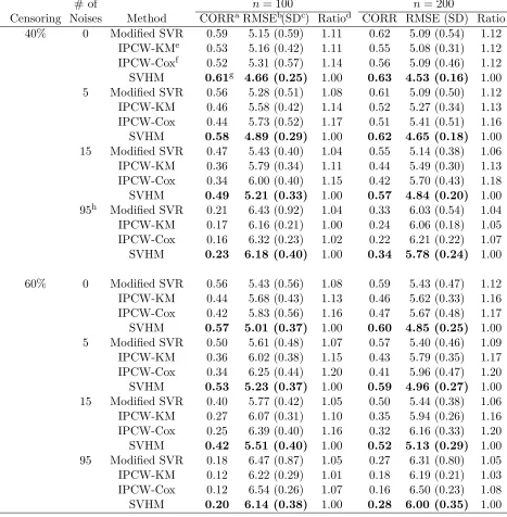
Table 1 and 2 give the average Pearson correlations and root mean square errors (RMSE)

{P

(Tb−T)2}1/2 based on the fitted event times and observed event timesT on the testing

data set. Larger correlation and smaller root mean squared error indicate better perfor-mance. The results show that SVHM outperforms the other methods for all the simulation cases and sample sizes. The advantages are not affected by including 5 or 15 noise variables, and the improvements become more evident when the censoring rate is 60% or the censoring distribution follows the accelerated failure time model. The columns of the average correla-tions show that the modified SVR has similar capability to capture the rank information as SVHM. However, it gives less accurate prediction of the exact event times as measured by the higher RMSEs. The IPCW methods have the worst performance, no matter using the Kaplan-Meier estimator or Cox model to estimate the censoring distribution, even when the censoring distribution follows the Cox model. The performances of all the methods are improved as the sample size increases from 100 to 200, and the proposed SVHM has the largest improvement with respect to the ratios of the average RMSEs. The RMSE of SVHM is significantly lower than the best competing method in all simulation settings in Table 1 and 2. Correlation between the risk scores and event times for SVHR is not significantly different from modified SVR, but in the first simulation setting it is significantly higher than two IPW-based methods except when there are 95 noise variables (Table 1). In the second simulation setting, difference between SVHR and IPW is smaller, with the former significantly greater for most cases withn= 200 (Table 2).

In conclusion, Table 1 shows that SVHM performs much better than Cox regression when the model assumption does not hold, and Table 2 shows that SVHM still maintains its advantage when the Cox proportional hazards assumption holds. This advantage may be due to that Cox model aims at maximizing the likelihood while SVHM directly aims at discriminating individual’s risk and prediction.

(17)

# of n= 100 n= 200

Censoring Noises Method CORRaRMSEb(SDc) Ratiod CORR RMSE (SD) Ratio

40% 0 Modified SVR 0.59 5.59 (0.60) 1.19 0.62 5.58 (0.58) 1.24

IPCW-KMe 0.40 5.60 (0.52) 1.20 0.45 5.45 (0.41) 1.21 IPCW-Coxf 0.43 5.80 (0.64) 1.24 0.50 5.62 (0.57) 1.25 SVHM 0.61g 4.68 (0.27) 1.00 0.64 4.49 (0.17) 1.00 5 Modified SVR 0.55 5.64 (0.60) 1.15 0.61 5.63 (0.57) 1.22

IPCW-KM 0.32 5.93 (0.47) 1.21 0.42 5.63 (0.44) 1.22

IPCW-Cox 0.33 6.17 (0.54) 1.26 0.44 5.87 (0.57) 1.27 SVHM 0.58 4.90 (0.35) 1.00 0.63 4.62 (0.20) 1.00 15 Modified SVR 0.46 5.73 (0.47) 1.10 0.54 5.55 (0.50) 1.15

IPCW-KM 0.21 6.12 (0.32) 1.18 0.31 5.86 (0.34) 1.22

IPCW-Cox 0.20 6.47 (0.46) 1.24 0.32 6.09 (0.47) 1.26 SVHM 0.48 5.20 (0.36) 1.00 0.57 4.82 (0.23) 1.00 95h Modified SVR 0.21 6.65 (0.89) 1.10 0.30 6.29 (0.47) 1.09

IPCW-KM 0.06 6.33 (0.21) 1.05 0.10 6.28 (0.14) 1.09

IPCW-Cox 0.08 6.59 (0.23) 1.09 0.11 6.61 (0.39) 1.15 SVHM 0.22 6.04 (0.32) 1.00 0.32 5.76 (0.25) 1.00

60% 0 Modified SVR 0.55 6.00 (0.54) 1.16 0.60 6.07 (0.42) 1.24

IPCW-KM 0.15 6.45 (0.41) 1.25 0.18 6.42 (0.37) 1.32

IPCW-KM 0.11 6.61 (0.34) 1.22 0.15 6.56 (0.32) 1.31

IPCW-KM 0.07 6.56 (0.30) 1.17 0.10 6.54 (0.24) 1.26

IPCW-KM 0.01 6.53 (0.26) 1.05 0.03 6.54 (0.20) 1.10

IPCW-Cox 0.02 6.87 (0.20) 1.10 0.04 6.86 (0.21) 1.15 SVHM 0.17 6.22 (0.24) 1.00 0.26 5.94 (0.25) 1.00 a

CORR, average value of correlations.

b

RMSE, average value of root mean square errors.

c _{Empirical standard deviation of the RMSE across 500 repetitions} d

Ratio, ratio of average root mean square errors between the method used and our method.

e _{IPCW-KM, IPCW using the Kaplan-Meier estimator for the censoring distribution.} f

IPCW-Cox, IPCW using the Cox model for the censoring distribution.

g _{Entries in boldface highlight the best performance method.} h

For the cases of 95 noises, the calculation of inverse weights in the IPCW-Cox method uses only five signal variables to fit the Cox model for the censoring times.

(18)

# of n= 100 n= 200

Censoring Noises Method CORRaRMSEb(SDc) Ratiod CORR RMSE (SD) Ratio

40% 0 Modified SVR 0.59 5.15 (0.59) 1.11 0.62 5.09 (0.54) 1.12

IPCW-KMe 0.53 5.16 (0.42) 1.11 0.55 5.08 (0.31) 1.12 IPCW-Coxf 0.52 5.31 (0.57) 1.14 0.56 5.09 (0.46) 1.12 SVHM 0.61g 4.66 (0.25) 1.00 0.63 4.53 (0.16) 1.00 5 Modified SVR 0.56 5.28 (0.51) 1.08 0.61 5.09 (0.50) 1.12

IPCW-KM 0.46 5.58 (0.42) 1.14 0.52 5.27 (0.34) 1.13

IPCW-KM 0.36 5.79 (0.34) 1.11 0.44 5.49 (0.30) 1.13

IPCW-Cox 0.34 6.00 (0.40) 1.15 0.42 5.70 (0.43) 1.18 SVHM 0.49 5.21 (0.33) 1.00 0.57 4.84 (0.20) 1.00 95h Modified SVR 0.21 6.43 (0.92) 1.04 0.33 6.03 (0.54) 1.04

IPCW-KM 0.17 6.16 (0.21) 1.00 0.24 6.06 (0.18) 1.05

IPCW-Cox 0.16 6.32 (0.23) 1.02 0.22 6.21 (0.22) 1.07 SVHM 0.23 6.18 (0.40) 1.00 0.34 5.78 (0.24) 1.00

60% 0 Modified SVR 0.56 5.43 (0.56) 1.08 0.59 5.43 (0.47) 1.12

IPCW-KM 0.44 5.68 (0.43) 1.13 0.46 5.62 (0.33) 1.16

IPCW-KM 0.36 6.02 (0.38) 1.15 0.43 5.79 (0.35) 1.17

IPCW-KM 0.27 6.07 (0.31) 1.10 0.35 5.94 (0.26) 1.16

IPCW-KM 0.12 6.22 (0.29) 1.01 0.18 6.19 (0.21) 1.03

IPCW-Cox 0.12 6.54 (0.26) 1.07 0.16 6.50 (0.23) 1.08 SVHM 0.20 6.14 (0.38) 1.00 0.28 6.00 (0.35) 1.00 a

CORR, average value of correlations.

b

RMSE, average value of root mean square errors.

c _{Empirical standard deviation of the RMSE across 500 repetitions} d

Ratio, ratio of average root mean square errors between the method used and our method.

e _{IPCW-KM, IPCW using the Kaplan-Meier estimator for the censoring distribution.} f

IPCW-Cox, IPCW using the Cox model for the censoring distribution.

g _{Entries in boldface highlight the best performance method.} h

For the cases of 95 noises, the calculation of inverse weights in the IPCW-Cox method uses only five signal variables to fit the Cox model for the censoring times.

(19)

for each method. Under the setting in Table 2 with 60% censoring rate, no noise variable and

n= 100, the correlations for the four methods are 0.52, 0.42, 0.40, and 0.55, respectively, and the RMSEs are 5.52, 5.76, 5.94, and 5.06.

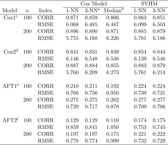
In our next simulation experiment, we compare SVHM with Cox model based analysis and explore 1-nearest-neighbor (1-NN) prediction and the average of 3-nearest-neighbors (3-NN) prediction. In the first setting we generate five discrete covariatesZ= (Z1, . . . , Z5) with

equal probability of taking each value: Z1takes values -5, -4, -2, -1 or 0;Z2takes values -1, 0

or 1;Z3takes integer values 1 to 10;Z4has a correlation of 0.5 withZ1and is also correlated with a random normal noise variableN(0,0.5), andZ5 has a correlation of 0.3 withZ1 and

is also correlated with a random uniform noise variable U(0,0.5). Similar to the previous simulations, the event times were generated from Cox proportional hazards model with true

β = (2,−1.6,1.2,−0.8,0.4)T and the exponential distribution with λ= 0.25 was assumed for the baseline cumulative hazard function Λ(t). The distribution of the censoring times followed Cox proportional hazards model with trueβ_c= (1,1,1,−2,−2)T and the baseline hazard rate was a constant. In the second setting, we generated Z1, ..., Z3 independently from U(0,1) and Z4 from a binary distribution with P(Z4 = 1) = P(Z4 = −1) = 0.5.

Furthermore, both the event times and censoring times were generated from accelerated failure time models with both main effects and interactions:

logT =−0.2−0.5Z1+ 0.5Z2+ 0.3Z3+ 0.5Z4−0.1Z1Z4−0.6Z2Z4+ 0.1Z3Z4+N(0,1),

logC = 0.5−0.8Z1+ 0.4Z2+ 0.4Z3+ 0.54−0.1Z1Z4−0.6Z2Z4+ 0.3Z3Z4+N(0,1).

The censoring ratio was around 30% in both settings. We experimented two sample sizes, 100 or 200, and two numbers of noise variables, 10 or 30.

The simulation results are summarized in Table 3. The same 1-NN or 3-NN method was applied to predict event times using the fitted scores derived from SVHM or Cox model. We can see that 1-NN performs slightly better than 3-NN in terms of a higher correlation and lower RMSE for both methods. In addition, when the event times were simulated from the Cox model, SVHM with 1-NN or 3-NN performs similarly to Cox model-based analysis. This is expected since proportional hazards assumption was satisfied for the Cox model based method. We also compared using 1-NN and 3-NN for prediction with using median survival times under a Cox model. We see 1-NN with SVHM or 1-NN with Cox model leads to superior performance than using median survival time. When the true model for the event times was accelerated failure time model (AFT), SVHM outperforms Cox model based analysis in terms of a higher correlation and lower RMSE. In the AFT model case, using the median survival time from the Cox model for prediction tends to be less accurate since the model assumption does not hold. Lastly, when the number of noise variables was 95, Cox model analysis did not converge in most simulations and thus the results were not included. In summary, results in Table 3 show that nearest neighbor based prediction rule performs better than using median survival time, and SVHM performs better than Cox model based methods when the model assumption does not hold.

4.2 PREDICT-HD Study

(20)

Cox Model SVHM

Model n Index 1-NN 3-NNa Medianb 1-NN 3-NN

Cox1c 100 CORR 0.871 0.859 0.866 0.863 0.851

RMSE 6.068 6.485 6.487 6.099 6.503

200 CORR 0.896 0.890 0.871 0.885 0.879

RMSE 5.755 6.168 6.226 5.781 6.186

Cox2d 100 CORR 0.841 0.831 0.839 0.854 0.844

RMSE 6.146 6.548 6.546 6.139 6.546

200 CORR 0.887 0.884 0.855 0.883 0.879

RMSE 5.760 6.209 6.273 5.761 6.214

AFT1e 100 CORR 0.210 0.211 0.192 0.224 0.224

RMSE 0.766 0.756 0.950 0.739 0.731

200 CORR 0.275 0.275 0.262 0.277 0.277

RMSE 0.720 0.717 0.879 0.709 0.706

AFT2f 100 CORR 0.129 0.129 0.110 0.174 0.175

RMSE 0.859 0.841 1.050 0.753 0.745

200 CORR 0.197 0.197 0.175 0.221 0.222

RMSE 0.778 0.774 0.999 0.732 0.729

a

Using mean of 3 nearest neighbors as predicted event time

b_{Using median survival time fitted from a Cox model as predicted event time.} c

T andCsimulated from Cox model with 10 noise variables.

d_T _and_C_{simulated from Cox model with 30 noise variables.} e

T andCsimulated from AFT model with 10 noise variables.

f

T andCsimulated from AFT model with 10 noise variables.

(21)

through a genetic testing of C-A-G expansion status at the IT15 gene (MacDonald et al., 1993). The availability of genetic testing and virtually complete penetrance of gene provides opportunity for early intervention. Currently a major research interest in HD is to combine salient clinical markers and biological markers sensitive enough to detect early indicators of patient disease diagnosis before evident clinical signs of HD emerge, and thus inform early interventions long before the clinical diagnosis. The hope of such early detection and intervention is to alter the disease course before substantial damage has occurred. The most promising markers thus far are brain imaging biomarkers and some cognitive markers which correlate with future clinical diagnosis (Paulsen, 2011; Paulsen et al., 2014).

(22)

5 15 25 35 45 55 65 75 0

1 2 3 4 5 6 7 8 9 10

Percentile as the cut point separating binary groups

Hazard ratio

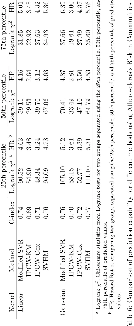
Linear Kernel

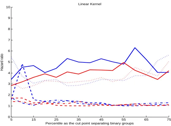
Figure 1: Hazard ratios comparing two groups separated using percentiles of predicted scores as cut points for PREDICT-HD data with linear kernel. Blue curves obtained from analyses with MRI imaging biomarkers and red curves without imaging biomarkers. Solid curve: SVHM; Dotted curve: Modified SVR; Dashed curve: IPCW-KM; Dashed-dotted curve: IPCW-Cox.

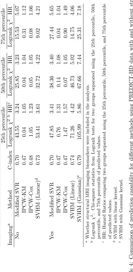
The analysis results are given in Table 4. SVHM improves over the other methods with respect to all the quantities for both linear kernel and Gaussian kernel, and the performances are similar using different kernels. For example, the logrank Chi-square statistics and hazard ratios of SVHM are much larger than the competing methods at most quantiles except at the right tail (e.g., over 65th percentile). A higher value of logrank Chi-square and a larger hazard ratio indicate greater difference between high risk and low risk subjects using a given percentile as a cut off value, and thus better discriminant ability of a risk score distinguishing high/low risk subjects. In addition, the predictions from IPCW cannot capture the trend of the original disease onset ages. Figure 1 complements the results in the table by plotting the hazard ratios comparing two groups separated using a series of percentiles of the predicted scores as cut points, and SVHM consistently has the largest hazard ratio across all percentiles among all methods. The improvement of SVHM increases at the higher percentiles, indicating that it is particularly effective in discriminating high risk subjects. This observation is consistent with our theoretical results which reveal that SVHM is optimal in separating the individual covariate-specific hazard function, h(t,x) given x, from the population average hazard function, ¯h(t).

(23)

(24)

Modified SVR yields coefficients in the same direction as SVHM, while two IPW methods give several coefficients in the opposite direction of other methods. SVHM suggests the top ranking markers with largest standardized effects to be the baseline total motor score and CAP score, which is consistent with the clinical literature on the importance of these markers on the diagnosis of HD (Zhang et al., 2011; Paulsen et al., 2014; Chen et al., 2014). The baseline total motor score as a measure of motor impairment appears to be more informative than CAP score in terms of predicting future HD diagnosis during the study. Several neuropsychological markers (Stroop color, Stroop word, SDMT) are predictive except for Stroop interference score. The coefficients from Cox model however, suggest that SDMT is not important, which is not consistent with the clinical literature (Paulsen, 2011; Paulsen et al., 2014). Note that SVHM gives psychiatric markers (SCL 90 depression, GSI, PST and PSDI) low weights which is consistent with clinical observations that the psychiatric markers are considered as noisy for predicting HD diagnosis due to reasons such as subjects may seek treatment for their psychiatric symptoms. In contrast, Cox model yields high weights for these markers which are deemed to be less informative.

In terms of neuroimaging markers, we see that pallidum, putamen, caudate, and thala-mus show relatively strong predictive ability of HD onset, while accumbens and hippocam-pus show low predictive ability. Comparing SVHM and Cox model analysis, note that SVHM provides coefficients with similar magnitude for imaging measures on the life and right side of the same brain region, but Cox model sometimes produces substantially dif-ferent results for left and right side. For example, left pallidum area is significant but not right pallidum area in Cox model. This observation suggests that SVHM may lead to more interpretable results especially for correlated variables. Another biomarker, cerebral spinal fluid, appears to be promising for predicting HD onset with a coefficient with moderate magnitude. To assess the added value of MRI imaging measures in terms of risk stratifica-tion, in Figure 1 we show the hazard ratio comparing high risk versus low risk group based on percentile split of the fitted scores obtained with and without imaging biomarkers. For SVHM with linear kernel, adding imaging measures leads to a larger hazard ratio and a greater difference between high and low risk groups at all percentiles, which demonstrates the ability of SVHM to extract information from imaging biomarkers and corroborates other findings suggesting their added values in predicting HD onset (Paulsen et al., 2014). When using Gaussian kernel for SVHM, we see further improvement of C-index and logrank chi-square statistics. Other methods such as modified SVR or IPCW do not show an ad-vantage from including imaging measures, which may suggest their limitations in handling correlated biomarkers.

4.3 ARIC Study

(25)

Variable Modified SVR IPCW-KM IPCW-Cox SVHM Cox modela (×10−1) (×10−2) (×10−3)

CAP 0.051 0.936 0.202 0.255 0.058

TOTAL MOTOR SCORE 0.280 -1.083 0.529 0.519 0.398*

SDMT -0.096 -0.411 0.076 -0.119 -0.190

STROOP COLOR -0.042 0.412 -0.038 -0.153 -0.160

STROOP WORD -0.227 0.488 0.188 -0.191 -0.217

STROOP INTERFERENCE 0.254 -0.432 -0.239 -0.000 0.328

TOTAL FUNCTIONAL CAPACITY -0.062 0.175 0.142 -0.072 0.007

UHDRS PSYCH 0.168 0.137 -0.280 0.155 0.228

SCL90 DEPRESS -0.285 -0.255 -0.132 -0.064 -0.618*

SCL90 GSI 0.316 -0.184 -0.182 0.007 0.618

SCL90 PST -0.108 -0.265 -0.246 -0.057 -0.268

SCL90 PSDI 0.099 -0.379 -0.249 0.103 0.035

FRSBE TOTAL -0.088 0.108 -0.136 0.112 0.115

Education Years 0.019 -1.057 0.349 -0.016 -0.053

Gender (Male) 0.178 -0.394 -0.202 0.376 0.344*

Right Putamen -0.009 -0.395 -0.376 -0.134 -0.038

Left Putamen -0.590 -0.165 -0.210 -0.116 -0.369

Right Pallidum -0.015 -0.490 -0.151 -0.225 -0.049

Left Pallidum -0.329 0.100 -0.189 -0.261 -0.626*

Right Caudate -0.830 0.655 -0.160 -0.147 -0.943*

Left Caudate 0.397 0.738 -0.265 -0.079 0.306

Right Accumbens 0.282 -0.214 -0.470 0.051 0.220

Left Accumbens -0.256 -0.568 -0.487 -0.057 -0.467*

Right Thalamus 0.099 -0.295 -0.710 0.172 0.260

Left Thalamus 0.258 -0.404 -0.636 0.219 0.138

Right Hippocampus 0.103 -1.152 -0.821 0.010 0.095

Left Hippocampus -0.130 -1.087 -0.847 -0.082 -0.128

Third Ventricle -0.101 1.071 0.841 -0.042 -0.046

Right Lateral Ventricle 0.140 2.794 1.409 -0.119 -0.016

Subcortical Gray Area 0.932 -0.868 -0.691 0.307 1.473*

Cerebral Spinal Fluid -0.268 0.116 0.954 -0.113 -0.104

a_{The estimates from Cox model with significant}_p_{-values (}_{p <}_{0.05) are marked with *.}

(26)

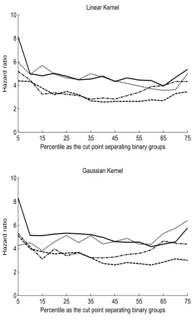
rate, left ventricular hypertrophy, bundle branch block, prevalent coronary heart disease, valvular heart disease, high-density lipoprotein, pack-years of smoking, and current and former smoking status. The analysis sample consists of 624 participants who are African-American males living in Jackson, Mississippi. Incident heart failure occurred in 133 men through 2005, with a median follow-up time 16.2 years. Among those participants who did not develop heart failure, 324 were administratively censored on December 31st, 2005. The analysis follows the same procedure as in Section 4.2. The results for prediction capability of different methods are given in Table 6. SVHM provides more accurate prediction than other methods using the linear kernel or Gaussian kernel. It also has higher logrank test statistic and hazard ratio comparing high risk versus low risk group using various percentiles of the predictive scores as cut off points (Figure 2).

In Table 7, we can see that all the risk factors have positive effects on the incident heart failure except high-density lipoprotein, serum albumin and former smoking status. Risk factors for incident heart failure with largest standardized effects include HDL, age, prevalent CHD, and serum albumin level. We also present estimated coefficients from a Cox proportional hazards model as comparison in Table 7. Most coefficients are comparable in terms of size. However, note that higher fasting glucose level appears to be protective of heart rate failure using Cox model, which is the opposite of the expected direction.

5. Concluding Remarks

In this paper, we propose a new statistical framework to learn risk scores for event times using right-censored data by support vector hazards machine. We propose to view the prediction of time-to-event outcomes from a counting process point of view to avoid compli-cations from specifying a censoring distribution. Asymptotically, we justify the associated universal consistency and learning rate through the structural risk minimization and show a natural link between the fitted decision function and the true hazard function: the fitted de-cision rule asymptotically minimizes the integrated difference between the covariate-specific hazard function and population average hazard function. Our theory shows that SVHM essentially compares events and non-events among the subjects at risk at each follow-up time; therefore, SVHM is sensitive to temporal difference between events and non-events which may not be reflected in either SVR or inverse weighted approaches. We also reveal a theoretical connection between SVHM and Cox partial likelihood function; the proposed method uses a hinge loss which should be robust to extreme observations in contrast to the exponential loss used in Cox partial likelihood. The simulation studies and real data applications demonstrate satisfactory results in finite samples with improved overall risk prediction accuracy in the presence of noise variables compared to other methods, espe-cially when the censoring rate is high and the distribution of censoring times is unknown. The improved performance of our method is due to introducing counting processes to repre-sent the time-to-event data, which leads to an intuitive connection of the method with both support vector machines in standard supervised learning and hazard regression models in standard survival analysis.

(27)

(28)

5 15 25 35 45 55 65 75 0

2 4 6 8 10

H

a

z

a

rd

r

a

ti

o

Linear Kernel

5 15 25 35 45 55 65 75

0 2 4 6 8 10

H

a

z

a

rd

r

a

ti

o

Gaussian Kernel

(29)

Covariate Normalizedβ Cox model a

Age (in years) 0.363 0.328 *

Diabetes 0.288 0.221 *

BMI (kg/m2) 0.150 0.136

SBP (mm of Hg) 0.172 0.178

Fasting glucose (mg/dL) 0.173 -0.093

Serum albumin (g/dL) -0.363 -0.273 *

Serum creatinine (mg/dl) 0.007 0.029

Heart rate (beats/minute) 0.124 0.125

Left ventricular hypertrophy 0.250 0.158 *

Bundle branch block 0.341 0.242 *

Prevalent CHD 0.330 0.216 *

Valvular heart disease 0.200 0.169 *

HDL (mg/dl) -0.287 -0.436 *

LDL (mg/dl) 0.016 0.051

Pack years of smoking 0.289 0.230 *

Current smoking status 0.210 0.022

Former smoking status -0.133 -0.232 *

a _{The estimates from Cox model with significant p-value (p-value}_<_{0.05) are}

marked with *.

(30)

through maximizing the Cox partial likelihood function, where the baseline hazard function is estimated to be non-continuous. Furthermore, due to the martingale property of the counting process, data from each time point can be viewed as independent in the learning method, despite that they may be from the same individual. Thus, we expect little efficiency loss even though some weighing scheme can be adopted to weight distinct risk sets differently over time.

In the current framework, the time-specific risk scoref(t,X) being considered includes a class of additive rules. They can be generalized to be fully nonparametric to learn dynamic risk profiles using a subject’s time-varying covariates under the current set up. However, this generalization may lose the similarity of formulation to the standard support vector machines and cause numerical instability in the optimization algorithm. These challenging issues will be further investigated in future work. One limitation of the current nonpara-metric framework not specifying the event distribution is that no straightforward prediction formulae using distribution exist. We used nearest neighbors to perform prediction and simulation studies show that using less closer neighbors (3-NN instead of 1-NN) has little influence on the results. In our simulation studies, we found that a training sample size of

n = 100 or n = 200 both yield stable estimation of correlation and RMSE (not sensitive to the choice of 1-NN or 3-NN). However, further work is needed to examine alternative prediction methods. Lastly, this work opens possibilities to use other powerful learning algorithms for binary and continuous outcomes to handle censored outcomes. For example, instead of using series of SVM to predict counting process as demonstrated here, other effective tools such as AdaBoosting and random forest can also be used. Gaussian process approaches (Barrett and Coolen, 2013) have been recently applied for survival data with competing risks so it will be interesting to compare SVHM with their approaches in terms of prediction performance and robustness.

Acknowledgments

(31)

Appendix A. SVHM Algorithm

In this section, we provide a detailed description of the SVHM algorithm:

Algorithm: SVHM for Censored Outcomes

Input: Training data (Xi, Ti∧Ci, Yi(tj), δNi(tj)) fori= 1,· · ·, n, j = 1,· · ·, m.

Step 1. Solve the quadratic programming problem:

max

γij

n X

i=1 m X

j=1

γijYi(tj)−

1 2

n X

i=1 n X

i0₌₁

m X

j=1 m X

j0₌₁

γijγi0_j0Y_i(t_j)Y_i0(t_j0)δN_i(t_j)δN_i0(t_j0)K(X_i,X_i0)

subject to: 0≤γij ≤wi(tj)Cn, n X

i=1

γijYi(tj)δNi(tj) = 0, i= 1, . . . , n, j= 1, . . . , m.

Denote the solutions as _bγij.

Step 2. Compute the risk scores for non-censored subjects in the training data as

b

g(Xs) = n X

i=1 m X

j=1 b

γijδNi(tj)K(Xs,Xi).

Step 3. Predicting event time of a future subject with covariatesxbyk -nearest-neighbor:

(a) Compute the risk score for this subject as _bg(x) =

Pn i=1

Pm

j=1bγijδNi(tj)K(x,Xi).

(b) Find k non-censored subjects in the training data whose risk scores are closest to_bg(x) and denote them as _bg(Xl) for l= 1,· · ·, k.

(c) Sort allgb(Xs) in descending order and denote the rank of bg(Xl) as rl

(d) Sort event times Ts of all non-censored subjects in ascending order. Find

therl-th event time and denote as Tl forl= 1,· · ·, k.

(e) The event time for this subject is predicted as Tb= 1_k P

lTl.

Output: For a subject with covariates x, predict risk score asg_b(x), and predict event time as Tb.

Appendix B. Proof of Theorems

In this section, we prove Theorem 3.1 and Theorem 3.2.

Proof (Theorem 3.1)

Since f∗(t,x) minimizes R(f), conditional X=x,f∗(t,x) also minimizes

E Z

Y(t)[1−f(t,X)]+dN(t)|X=x

+

Z

E(Y(t)[1 +f(t,X)]+|X=x)

E(Y(t)) E(dN(t)). (A.1) Clearly, the valuef∗(t,x) should belong to the interval [−1,1], because otherwise truncation of f at−1 or 1 gives a lower value. Assuming−1≤f(t,x)≤1, (A.1) becomes

Z

E(Y(t)|X=x){h(t,x) + ¯h(t)}dt−

Z

(32)

where recall thath(t,x) is the conditional hazard rate ofT =tgivenX=xand ¯h(t) is the population average hazard at time t,

¯

h(t) = E[dN(t)]/dt

E[Y(t)] =E[h(t,X)|Y(t) = 1]. Therefore, one optimal decision function minimizingRL(f) is

f∗(t,x) = sign{h(t,x)−¯h(t)}.

On other hand, we note

R₀(f) =

Z

I[f(t,x)≤0]E(Y(t)|X=x)h(t,x)dt+

Z

I[f(t,x)≥0]E(Y(t)|X=x) ¯h(t)dt.

Thus, any decision function has the same sign as (h(t,x)−¯h(t)) minimizesR0(f) sof∗(t,x)

minimizesR₀(f). Finally, under the optimal rulef∗(t,x), the minimal value of the weighted 0-1 risk is given as

R0(f∗) = E Z

E(Y(t)|X=x) min{h(t,x),¯h(t)}dt

= 1

2E

Z

E(Y(t)|X=x){h(t,x) + ¯h(t)− |h(t,x)−¯h(t)|}dt

= P(T ≤C)−1

2E

Z

E(Y(t)|X=x)|h(t,x)−¯h(t)|dt

.

To show the last inequality in Theorem 3.1, we note hat for −1≤f(t,x)≤1,

R(f) = E Z

E(Y(t)|X=x){h(t,x) + ¯h(t)}dt−

Z

f(t,x)E(Y(t)|X=x){h(t,x)−¯h(t)}dt

= 2P(T ≤C)−E Z

f(t,x)E(Y(t)|X=x){h(t,x)−¯h(t)}dt

,

and

R(f∗) = 2P(T ≤C)−E Z

sign{h(t,x)−λn¯(t)}E(Y(t)|X=x){h(t,x)−¯h(t)}dt

.

Thus,

R(f)− R(f∗) = E Z

E(Y(t)|X=x)sign{h(t,x)−¯h(t)} −f(t,x) × {h(t,x)−¯h(t)}dt

= E

Z

E(Y(t)|X=x)f(t,x)−sign{h(t,x)−h¯(t)}

× |h(t,x)−¯h(t)|dt

On the other hand, for the risk function based on the 0-1 loss, we have

R0(f)− R0(f∗)

= E

Z

E(Y(t)|X=x) I[f(t,x)≤0]h(t,x) +I[f(t,x)≥0]¯h(t)−min{h(t,x),¯h(t)} dt

= E

Z

E(Y(t)|X=x)h(t,x)−¯h(t)

×I {h(t,x)−¯h(t)}sign{f(t,x)}<0

dt