Fused Lasso Approach in Regression Coefficients Clustering
– Learning Parameter Heterogeneity in Data Integration
Lu Tang [email protected]
Peter X.K. Song [email protected]
Department of Biostatistics University of Michigan Ann Arbor, MI 48109, USA
Editor:Hui Zou
Abstract
As data sets of related studies become more easily accessible, combining data sets of similar studies is often undertaken in practice to achieve a larger sample size and higher power. A major challenge arising from data integration pertains to data heterogeneity in terms of study population, study design, or study coordination. Ignoring such heterogeneity in data analysis may result in biased estimation and misleading inference. Traditional techniques of remedy to data heterogeneity include the use of interactions and random effects, which are inferior to achieving desirable statistical power or providing a meaningful interpreta-tion, especially when a large number of smaller data sets are combined. In this paper, we propose a regularized fusion method that allows us to identify and merge inter-study homogeneous parameter clusters in regression analysis, without the use of hypothesis test-ing approach. Ustest-ing the fused lasso, we establish a computationally efficient procedure to deal with large-scale integrated data. Incorporating the estimated parameter ordering in the fused lasso facilitates computing speed with no loss of statistical power. We con-duct extensive simulation studies and provide an application example to demonstrate the performance of the new method with a comparison to the conventional methods.
Keywords: Fused lasso, Data integration, Extended BIC, Generalized Linear Models
1. Introduction
Combining data sets collected from multiple studies is undertaken routinely in practice to achieve a larger sample size and higher statistical power. Such information integration is commonly seen in biomedical research, for example, the study of genetics or rare diseases where data repositories are available. The motivation of this paper arises from the con-sideration of data heterogeneity during data integration. Although data integration has different meanings, in here, we consider the concatenation of data sets of similar studies over different subjects, where the number of integrated data sets can be very large.
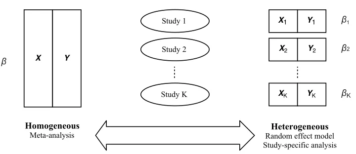
Figure 1: Homogeneous assumption (left) versus heterogeneous assumption (right).
from multiple similar studies are combined (Lohmueller et al., 2003; Sullivan et al., 2000). Discrepancies in treatment effect or trait-gene association may arise due to the differences in facilities, practices and patient characteristics across studies, albeit the adjustment of confounding (Leek and Storey, 2007). The parameter heterogeneity introduced in data in-tegration compromises the power of the larger sample size and may even lead to biased results and misleading scientific conclusions. Thus, counterintuitively, the model obtained from the combined studies may not serve as a proper prediction model for each individual study in the case of heterogeneous study populations.
Traditional treatments of parameter heterogeneity are not optimal. Meta-analysis meth-ods such as combining summary statistics (Glass, 1976), estimating functions (Hansen, 1982; Qin and Lawless, 1994) orp-values functions (Xie et al., 2012) are built upon the assump-tion of complete parameter homogeneity, as shown in the left panel of Figure 1. This as-sumption is hardly valid in practice. When individual participant data from multiple data sets are available, a retreat to the classical meta-analysis methods is necessary, because in this case assessing the assumption of inter-study homogeneity becomes possible. The two most common approaches to handling parameter heterogeneity include (i) specifying study-specific effects by including interaction terms between study indicator and covariates (e.g., Lin et al. (1998)), and (ii) utilizing random covariate effects by allowing variations across studies as random variables (e.g., DerSimonian and Kacker (2007)). Both approaches essentially assume fully heterogeneous covariate effects, namely, each study having its own set of regression coefficients, as shown in the right panel of Figure 1.
When study-specific effects are of interest, the interaction-based formulation may lead to over-parameterization, which impairs statistical power. The most straightforward way to reduce the number of parameters is to identify clusters of homogeneous parameters through exhaustive tests for the differences between every pair of study-specific coefficients. However, when the number of data sets is large, the use of hypothesis testing to determine parameter clusters becomes untrackable in addition to the multiple-testing problem. One may draw different or even conflicting conclusions due to different orders of hypotheses performed.
to the following two essential yet related analytic tasks: (i) to assess the inter-study het-erogeneity, so to determine an appropriate form of parsimonious parameterization in model specification; and (ii) to identify and merge groups of homogeneous parameters for bet-ter statistical power for paramebet-ter estimation and inference based on a more parsimonious model. Along the idea of lasso shrinkage estimator (Tibshirani, 1996), fused lasso methods (Tibshirani et al., 2005; Friedman et al., 2007; Yang et al., 2012) have been introduced to achieve covariate grouping, where covariate adjacencies are naturally defined by a metric of time, location or network structure. In our problem of data integration, there does not exist a natural metric to define the ordering of regression coefficients from different studies. Shen and Huang (2010) proposed the grouping pursuit via penalization of all pairwise coefficient differences in a single study, where covariate orderings are not considered. To reduce the computational burden in the all-pairs based regularization, Wang et al. (2016) and Ke et al. (2015) used the initial coefficient estimates to establish certain ordering and then to define parameter adjacencies. However, most of these studies have been entirely focusing on a single cohort of subjects from a single study. For example, Shin et al. (2016) proposed to fuse regression coefficients of different loss functions obtained from a single study, such as coefficients from different quantile regression models. Limited publication of fusion learning and grouping pursuit has been available in the literature, except Wang et al. (2016), to assess the differences and similarities among regression coefficients across multiple studies in the scenario of data integration.
In this paper, we propose an agglomerative clustering method for regression coeffi-cients in the context of data integration, named as theFused Lasso Approach in Regression Coefficients Clustering (FLARCC). FLARCC is proposed to identify heterogeneity pat-terns of regression coefficients across studies (or data sets) and to provide estimates of all regression coefficients simultaneously. It is interesting to draw a connection between our method and Pan et al. (2013) where they consider a classic clustering problem of in-dividual responses by pairwise coefficient fusion via penalized regression. Their method aims at clustering subjects, while our method focuses on clustering regression coefficients across multiple data sets, and these two methods coincide only in a special case where each study is composed of only one subject. FLARCC achieves clustering of study-specific effects by penalizing the `1-norm differences of adjacent coefficients, with adjacency de-fined by the estimated ranks. Our method extends the bCARDS method in Ke et al. (2015) from one study to multiple studies as well as from the linear model to the gen-eralized linear models, and focuses on simultaneous clustering of regression coefficients of individual covariates from multiple studies in data integration. An R package metafuseis created as part of our methodology development to perform the proposed integrated data analysis which can be downloaded from the Comprehensive R Archive Network (web link https://cran.r-project.org/web/packages/metafuse).
scheme, these two extreme cases above correspond to the start and end of an agglomerative clustering, respectively; however, the reality is believed to reside in between. Analogous to dendrograms in the hierarchical clustering, we propose a new tree-type graphic display, named asfusogram, which presents tree-based coefficient clusters according to solution paths obtained from FLARCC. The selection of optimalλpertains to pruning of clustering trees, which can be based on certain model selection criterion. We use the extended Bayesian information criterion (EBIC) proposed by Chen and Chen (2008) as our model selection criterion and show that EBIC exhibits better performance than BIC when the number of studies (or data sets) is large. In addition, we propose a scaling strategy to “harmonize” solution paths by covariate-wise adaptive weights to allow flexible tuning, which further improves the clustering performance.
The rest of this paper is organized as follows. Section 2 describes FLARCC in detail under the generalized linear models (GLM) framework. Section 3 presents the theoretical properties of the proposed method (with technical proofs presented in the Appendix). Sec-tion 4 discusses the interpretaSec-tion and selecSec-tion of the tuning parameter. In SecSec-tion 5, we use simulation studies to evaluate the performance of our method. A real data analysis is given in Section 6 with interpretation of coefficient estimates and illustration offusograms. Discussion and concluding remarks are in Section 7.
2. Method of Parameter Fusion
In this section, we present the method and algorithm of FLARCC.
2.1 Notations and Method
We start by introducing necessary notations. Throughout this paper, i, j and k are used to index subject, covariate and study, respectively. For instance,Xj,k(i) denotes the measure-ment of thejth covariate from theith individual from studyk, andYk(i)is the measurement of a response variable from theith individual from study k. The total number of studies is denoted asKand the number of covariates involved isp. The sample size for studykisnk,
k = 1, . . . , K, and the combined sample size is N = PK
k=1nk. The collection of all coeffi-cients (covariates-wise) is denoted asβ= (β1,>
·
,β>2,·
, . . . ,βp,>·
)>withβj,·
= (βj,1, . . . , βj,K)>forj = 1, . . . , p. An indicator vectorc = (c1, . . . , cp)> is used to flag heterogeneous
covari-ates, namely if the jth covariate is treated as heterogeneous (i.e., all different coefficients acrossK studies) thencj = 1 and as homogeneous (a common coefficient acrossK studies) otherwise. Thus cj = 0 for some j ∈ {1, . . . , p} implies that coefficient vector βj,
·
reduces to a common scalar parameter βj for all K studies.For illustration, let us consider a simple scenario of c = (1,1,0, . . . ,0)>, in which the first two covariates are set as heterogeneous and the remaining p−2 covariates are set as homogeneous. The resulting coefficient vector is β= (β1,>
·
,β2,>·
, β3, . . . , βp)>.Then the corresponding design matrix X can be written asX =
X1,1 X2,1 X3,1 . . . Xp,1
. .. . .. ... . .. ...
X1,K X2,K X3,K . . . Xp,K
whereXj,k = (Xj,k(1), . . . , Xj,k(n))>,j= 1, . . . , p,k= 1, . . . , K. The specification ofcis can be dependent on the study interest. For example, in a multi-center clinical trial where we be-lieve that the differences between the services provided across centers are non-negligible, but the study participants are similar, we can specify the clinic-related variables (e.g., treatment and cost) to be heterogeneous and the patient-related variables (e.g., age and gender) to be homogeneous. In addition, the specification ofccan be dependent on preliminary marginal analysis of the homogeneousness of each variable, such as tests for random effects. When the homogeneousness of a covariate is unclear, we suggest specifying it as heterogeneous rather than homogeneous.
Under the assumption that both within-study and between-study samples are indepen-dent, for any c = (c1, . . . , cp)> with cj ∈ {0,1}, j = 1, . . . , p, the initial estimate of β, which gives the starting level of clustering (i.e., λ = 0), can be consistently estimated by the maximum likelihood estimator
ˆ
β= argmax β∈R(K×p)
1
K
K
X
k=1 1
nk
logLk(β), (1)
whereLk(β) =Qni=1k L (i)
k (β), k= 1, . . . , K are the study-specific likelihoods from the given
GLMs. For the purpose of parameter grouping and fusion, we propose the regularized maximum likelihood estimation forβ by minimizing the following objective function:
min β∈R(K×p)
−1
K
K
X
k=1 1
nk
logLk(β) +P(β)
!
, (2)
where P(β) is a penalty function of certain form. Here we adopt weighting n1
k to balance
the contribution from each study so to avoid the dominance of large studies. Other types of weighting schemes may be considered to serve for different purposes, such as the inverse of estimated variances of initial estimates, which helps to achieve better estimation precision. To achieve parameter fusion, Shen and Huang (2010) proposed the grouping pursuit algorithm, which specifies the sum of `1-norm differences of all study-specific coefficient pairs among individual heterogeneous coefficient vectorsβj,
·
, wherecj = 1, as the penalty:Pλ(β) =λ p
X
j=1
cj
K−1
X
k=1 K
X
k0>k
|βj,k−βj,k0|,
with λ ≥ 0. In this penalty, there are K2
terms of pairwise differences for each hetero-geneous covariate and the total number of terms increases by an order of O(K2), given p
fixed. This penalty contains many redundant constraints and imposes great computational challenges as pointed out in Shen and Huang (2010) and Ke et al. (2015).
Following arguments in Wang et al. (2016) and Ke et al. (2015), we develop the method of FLARCC by a simplified penalty function that uses the information on the ordering of coeffi-cients. For thejth covariate, letUj = (Uj,1, . . . , Uj,K)>be the ranking with no ties ofβj,
·
=(βj,1, . . . , βj,K)>, from the smallest to the largest. Specifically,Uj,k =PKk0=11{βj,k0 ≤βj,k}
rule according to k to ensure rank uniqueness. Then, the fusion penalty in FLARCC with parameter orderingsUj,j= 1, . . . , p, takes the form:
Pλ(β) =λ p
X
j=1
cjνj
K−1
X
k=1 K
X
k0>k
µj,k,k01{|Uj,k−Uj,k0|= 1}|βj,k−βj,k0|, (3)
where the constraints occur effectively only on adjacent ordered pairs. Clearly, the penalty in (3) only involves K−1 terms for each case of cj = 1, which is of an order O(K), given
p fixed. Theνj’s andµj,k,k0’s in (3) are weights. Following Zou (2006), we choose adaptive
weights ˆµj,k,k0 = 1/|βˆj,k−βˆj,k0|r, r >0, so that parameters with smaller difference will be
penalized more than those with larger differences. Similarly, for a group of parametersβj,
·
=(βj,1, . . . , βj,K)>,νj is an adaptive weight to characterize the degree of heterogeneousness of
βj,
·
. Specifically, in this paper we let ˆνj = 1/|βˆj,(K)−βˆj,(1)|s, the inverse of the range of the estimates, with s ≥ 0; when a covariate is homogeneous, the differences of study-specific coefficients will be penalized more than those that are heterogeneous. In this way, we can “harmonize” solution paths so to greatly improve the performance by a single tuning parameter. We compare s = 0 and s = 1 in the simulation experiments and show in Section 5 that the introduction of such group-wise weights νj, j = 1, . . . , p, gives rise to improvement on the performance of identifying homogeneous covariates whenK and pare large.A sparse version of FLARCC can also be achieved by including the traditional lasso penalty in (3) for covariate selection. In order to minimize the interference between fusion and sparsity penalties, we only encourage sparsity for the coefficient closest to zero in
each βj,
·
= (βj,1, . . . , βj,K)>, for j = 1, . . . , p. Similar to the definition of Uj, let Vj =(Vj,1, . . . , Vj,K)>be the ranking with no ties, from the smallest to the largest, of the absolute
values of βj,
·
, i.e., (|βj,1|, . . . ,|βj,K|)>. First we calculate Vj by Vj,k =PK
k0=11{|βj,k0| ≤
|βj,k|}, then we resolve the ties inVj by the first-occurrence-wins rule according tok. Thus we can extend (3) to achieve variable selection by the following penalty function:
Pλ,α(β) =λ
p
X
j=1
cjνj
K−1
X
k=1 K
X
k0>k
µj,k,k01{|Uj,k−Uj,k0|= 1}|βj,k−βj,k0|
+αλ
p
X
j=1 K
X
k=1
µj,k1{Vj,k= 1}|βj,k|,
(4)
whereα≥0 is another tuning parameter that controls the relative ratio between fusion and sparsity penalties, and ˆµj,k = 1/|βˆj,k|r. The sparsity penalty, although only enforced on the smallest coefficient in absolute value of βj,
·
, is capable of shrinking a group of coefficients to zero when combined with the fusion penalty.In practice, the weights (νj,µj,k,k0 andµj,k) and the parameter orderings (Uj andVj) are
2.2 Algorithm
Optimization problem (2) with P(β) =Pλ,α(β) given in (4) can be carried out by a lasso regression through suitable reparameterization. Let the ordered coefficients of βj,
·
in an ascending order based on ranking Uj be (βj,(1), . . . , βj,(K))>, j = 1, . . . , p. For the jth covariate, consider a set of transformed parameters θj,·
= (θj,1, . . . , θj,K)> defined byθj,1 =βj,k, fork s.t. Vj,k = 1;
θj,k =βj,(k)−βj,(k−1), fork= 2, . . . , K. Then the Pλ,α(β) in (4) can be rewritten as
Pλ,α(θ) =λ
p
X
j=1 K
X
k=1
ωj,k|θj,k|, (5)
where
ˆ
ωj,k =
α 1
|θˆj,1|r, ifk= 1
cj|PK 1
k0=2θˆj,k0|s
1
|θˆj,k|r, ifk= 2, . . . , K,
(6)
forj= 1, . . . , p. Since no ties are allowed in the parameter ordering of FLARCC, one-to-one
transformation exists between β = (β>1,
·
,β2,>·
, . . . ,β>p,·
)> and θ = (θ>1,·
,θ2,>·
, . . . ,θp,>·
)> by suitable sorting matrix S and reparameterization matrix R; that is, θ = RSβ and β = (RS)−1θ with bothS and Rbeing full-rank square matrices. Thus, a solution to the fused lasso problem can be obtained equivalently by solving a routine lasso problem with respect to coefficient vector θ and a transformed design matrix X(RS)−1. As aforementioned, the estimated parameter ordering is used to constructS. It is obvious that the constraint in (5) is convex, thus FLARCC does not suffer from multiple local minimal issue. The optimization is done using R packageglmnet(version 2.0-2) (Friedman et al., 2010), which accommodates GLMs with Gaussian, binomial and Poisson distributions.3. Large-sample Properties
First we present the oracle property of our method when the parameter ordering is known, then we prove that the same large-sample properties are preserved when consistently esti-mated parameter ordering is used. Here we assume K is fixed. Theorems will be stated under the setting of all coefficients being heterogeneous, i.e., c = (1, . . . ,1)>. The large-sample theories for other specification ofc can be established as a special case.
Denote the true parameter values as β∗ and θ∗. Let the collection of true parameter orderings of all covariates and their absolute values beW ={Uj,Vj}pj=1, and the estimated orderings based on the root-nconsistent estimator ˆβfrom (1) as ˆW ={Ujˆ ,Vjˆ }pj=1. Denote the FLARCC estimator of θ∗ as ˆθW when W is known, and ˆθWˆ when the estimated parameter ordering ˆW is used. LetA=Sp
j=1{Aj}be the index set of nonzero values inθ∗, whereAj ={(j, k) :θj,k∗ 6= 0}, andAcbe the complement ofA. Thus,θ∗ can be partitioned into two subsets, the true-zero setθA∗c and the nonzero set θA∗. Similarly, let ˆAW and ˆA
ˆ W
be the index sets of nonzero elements in ˆθW and ˆθWˆ, respectively. Let n = min 1≤k≤Knk,
N =PK
Theorem 1 Suppose that tuning parameter λN satisfiesλN/
√
N → 0 and λNN(r−1)/2 →
∞. Then under some mild regularity conditions (see Appendix A), the FLARCC estimator ˆ
θW based on the true parameter ordering W satisfies
(i) (Selection Consistency) limnP( ˆAW =A) = 1;
(ii) (Asymptotic Normality) √N( ˆθAW −θA∗) → Nd (0,I11−1) as n → ∞, where I11 is the submatrix of Fisher information matrix I corresponding to set A.
Theorem 1 states that when the coefficient orderingsW ofβ is known, under mild reg-ularity conditions, the FLARCC estimator ˆθW enjoys selection consistency and asymptotic normality. The proof of Theorem 1 follows Zou (2006) and is given in Appendix A. Now we present Theorem 3, which states that the same properties of Theorem 1 hold for ˆθWˆ, the FLARCC estimator of θ∗ based on the estimated parameter ordering ˆW. In effect, Theorem 3 is a consequence of the following lemma.
Lemma 2 If βˆ is a root-n consistent estimator of β, then limnP( ˆUj = Uj) = 1 and limnP( ˆVj =Vj) = 1 for j= 1, . . . , p.
The proof of Lemma 2 is given in Appendix A. Lemma 2 implies that the parameter ordering can be consistently estimated. Using Lemma 2, we are able to extend the properties of ˆθW in Theorem 1 to the proposed FLARCC estimator ˆθWˆ .
Theorem 3 Suppose thatλN/
√
N →0andλNN(r−1)/2 → ∞. Let the estimated parameter ordering Wˆ be the ranks from a root-n initial consistent estimator βˆ. Under the same regularity conditions of Theorem 1, the FLARCC estimatorθˆWˆ satisfies
(i) (Selection Consistency) limnP( ˆAWˆ =A) = 1;
(ii) (Asymptotic Normality) √N( ˆθAWˆ −θA∗) → Nd (0,I11−1) as n → ∞, where I11 is the submatrix of Fisher information matrix I corresponding to set A.
The proof of Theorem 3 is given in Appendix A. The asymptotic normality for ˆβ can also be derived by a simple linear transformation.
4. Tuning Parameter
In this section, we provide interpretation of the tuning parameterλand discuss the selection criteria used for selectingλ.
4.1 Interpretation of νj’s
Intuitively speaking, the study-specific coefficients of a homogeneous covariate tend to be fused at a smallλvalue, sayλ1, but the fusion of a heterogeneous covariate requires another
be empty. For example, when λ2 < λ1 in the above case, no single λ is able to correctly cluster both sets of parameters. The introduction of νj’s in (4) creates larger separation between homogeneous and heterogeneous groups, so that the range for λ to identify the correct clustering pattern for all covariates is better established than the case with s= 0, namely no use of weightingνj’s. When the number of covariatespis large, νj plays a more important role in harmonizing solution paths across covariates, and the performance will be greatly improved by simultaneous tuning via a singleλ.
4.2 Model Selection
In the current literature, the tuning parameterλmay be selected by multiple model selection criteria, such as Bayesian information criterion (BIC) (Schwarz, 1978) and generalized cross-validation (GCV) (Golub et al., 1979). In this paper, we consider the widely used BIC and its modification, extended BIC, i.e., EBIC (Chen and Chen, 2008; Gao and Song, 2010), which has showed the benefit of achieving sparse solutions.
Following the derivation of BIC for weighted likelihoods in Lumley and Scott (2015), the conventional BIC for FLARCC is defined as follows:
BICλ =−2
K
X
k=1 ¯
n
nk
logLk( ˆβ(λ)) + df( ˆβ(λ)) log(N), (7)
where ¯n=N/K is the average sample size per study,Lk(β) is the study-specific likelihood, ˆ
β(λ) is the estimation of β at tuning parameter valueλ, and df( ˆβ(λ)) =Pp
j=1df( ˆβj,
·
(λ)) is the total number of distinct parameters in ˆβ(λ). The study-specific log-likelihoods for three most common models are listed below:Normal: logLk( ˆβ(λ))∝ −
nk
2 log
(nk X
i=1
Yk(i)−Xk(i)>β(ˆ λ)
2
/nk
)
;
Logistic: logLk( ˆβ(λ))∝ nk
X
i=1
n
Yk(i)Xk(i)>β(ˆ λ)−log1 +eXk(i)>βˆ(λ)
o
;
Poisson: logLk( ˆβ(λ))∝ nk
X
i=1
n
Yk(i)Xk(i)>β(ˆ λ)−eXk(i)>βˆ(λ)
o .
To improve the BIC by further controlling model size and encouraging sparer models, we adapt the EBIC for FLARCC, which takes the following form:
EBICλ =−2
K
X
k=1 ¯
n
nk
logLk( ˆβ(λ)) + df( ˆβ(λ)) log(N) + 2γlog p
X
j=1
K
df( ˆβj,
·
(λ))
, (8)
In a view of hierarchical clustering, the solution path of each covariate can be thought of as a hierarchical clustering tree. For thejth covariate,λ= 0 corresponds to the bottom of the clustering tree; and λ=λF use,j, the smallestλvalue to achieve complete parameter fusion, corresponds to the top of the clustering tree. The completely heterogeneous model corresponds to the position on the solution path atλ= 0 and the completely homogeneous model corresponds to the model atλ=λF use:= max
1≤j≤pλF use,j.
5. Simulation Studies
This section presents results from two simulation experiments. The first simulation com-pares the performance of FLARCC under different GLM regression models. The second simulation is a more complicated scenario with largeKand more non-important covariates, where covariate selection is also of interest.
5.1 Simulation Experiment 1
The first simulation study aims to assess the performance of our method for different GLM regression models. For this, we consider combining data sets fromK= 10 different studies with, for simplicity, equal sample size n1 =· · · =n10 = 100. Data are simulated from the following mean regression model:
h{E(Yk(i))}=β1,kX1,k(i)+β2,kX2,k(i)+β3,kX3,k(i), i= 1, . . . ,100, k= 1, . . . ,10,
where the true coefficient vectors have the following clustering structures:
β1,
·
= (0, . . . ,0| {z }
10 )>;
β2,
·
= (0, . . . ,0| {z }
5
,1, . . . ,1
| {z }
5 )>;
β3,
·
= (−1, . . . ,−1| {z }
3
,0, . . . ,0
| {z }
4
,1, . . . ,1
| {z }
3 )>.
The true values inβ2andβ3 are heterogeneous, while the true values inβ1are homogeneous across studies. The three covariates are correlated with exchangeable correlation of 0.3 and marginally distributed according to the standard normal distributions,N(0,1). Three types of GLM regression models are considered: linear model for continuous normal outcomes (with errors simulated fromN(0,1)), logistic model for binary outcomes and Poisson model for count outcomes.
To evaluate the performance of FLARCC to correctly detect patterns of all covariates, we assume all covariates are heterogeneous across studies with no prior knowledge on clus-tering structure of any covariate. Intercept is fitted and assumed to be homogeneous. No sparsity penalty is applied on the covariates (i.e.,α= 0) in this simulation experiment. Co-efficients of all three covariates are fused simultaneously, and the optimal tuning parameter
Method
β βˆsize λ˜F use,j
Sensi- Speci- MSE whenλ= (˜λopt) tivity ficity λopt λF use 0
Linear: continuous response
s= 0
(0.154)
β1 1.067 0.111 0.974 – 0.001 0.002 0.012 β2 2.075 1.275 0.982 1.000 0.003 0.253 0.012 β3 3.081 1.368 0.982 1.000 0.004 0.603 0.012
s= 1
(0.349)
β1 1.006 0.080 0.998 – 0.001 0.002 0.012 β2 2.058 1.584 0.986 1.000 0.003 0.253 0.012 β3 3.123 1.972 0.974 1.000 0.004 0.603 0.012
Logistic: binary response
s= 0
(0.066)
β1 1.270 0.064 0.898 – 0.010 0.005 0.070 β2 2.572 0.318 0.819 0.963 0.047 0.268 0.087 β3 3.682 0.437 0.784 0.964 0.069 0.607 0.091
s= 1
(0.112)
β1 1.075 0.050 0.972 – 0.007 0.005 0.069 β2 2.478 0.414 0.837 0.952 0.052 0.268 0.088 β3 3.912 0.711 0.749 0.971 0.064 0.607 0.091
Poisson: count response
s= 0
(0.187)
β1 1.087 0.129 0.976 – 0.001 0.005 0.008 β2 2.084 1.751 0.984 1.000 0.001 0.271 0.008 β3 3.076 1.885 0.986 1.000 0.002 0.659 0.008
s= 1
(0.433)
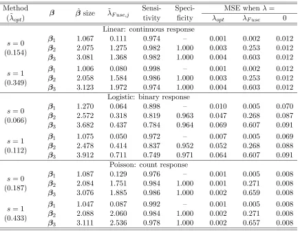
β1 1.047 0.087 0.992 – 0.001 0.005 0.008 β2 2.088 2.060 0.984 1.000 0.002 0.271 0.008 β3 3.111 2.536 0.978 1.000 0.002 0.657 0.008 Table 1: Results of simulation experiment 1 for FLARCC when scaling weight parameter
s = 0 and s = 1 with λ selected by EBIC, for the linear, logistic and Poisson models. Tuning parameters are reported in log scale, i.e., ˜λ= log10(λ+ 1). Results are summarized from 1,000 replications.
the proportion of unequal coefficients pairs that are correctly identified; however, specificity is not defined for homogeneous covariates which have no unequal coefficient pairs. In addi-tion, we calculate the mean squared error (MSE) for each ˆβj,
·
across all K studies, defined as MSEj =PKk=1( ˆβj,k−βj,k)2/K, j= 1, . . . , p,and compare with the MSE of each estimate based on homogeneous model (λ=λF use) and heterogeneous model (λ= 0).regression coefficients in the logistic model are larger than in the linear and Poisson models, given the same coefficient setting. Therefore, the estimated parameter ordering for which our method is based on may be less accurate. For the logistic regression, increasing sample sizes is one of the possible ways to improve the performance. The performance difference between scaling weight parameters= 0 ands= 1 in (4) is small in this case because of the relatively small number of covariates p= 3. Additionally, sinceK is small in this case, the optimalλselected by BIC and EBIC are very close, thus we only display results based on EBIC. As p and K become larger, FLARCC will increasingly benefit from the additional weightsνj (i.e.,s= 1) and EBIC, as will be shown in Section 5.2. A sensitivity analysis to investigate how the initial ordering affect the performance of FLARCC is conducted, with results shown in Appendix B. We show that when the initial parameter ordering is slightly distorted, our method still achieves satisfactory performance.
5.2 Simulation Experiment 2
The second simulation study aims to evaluate the performance of FLARCC in a more challenging setting. More specifically, we consider data sets fromK = 100 studies, each with a sample size 100, totaling 10,000 subject-level observations. Comparing to the previous setting, we increase the number of covariates and reduce the gaps between heterogeneous coefficients. For each study, we simulate data from the following linear regression model:
E(Yk(i)) =
8
X
j=1
βj,kXj,k(i), i= 1, . . . ,100, k= 1, . . . ,100.
The signals are set sparse; only the first four covariates with coefficient vectors, β1 to β4, are influential toY with the true clustered effect patterns given as follows:
β1,
·
= (0, . . . ,0| {z }
50
,0.5, . . . ,0.5
| {z }
50
)>,
β2,
·
= (−0.5, . . . ,−0.5| {z }
30
,0, . . . ,0
| {z }
40
,0.5, . . . ,0.5
| {z }
30
)>,
β3,
·
= (−0.5, . . . ,−0.5| {z }
25
,0, . . . ,0
| {z }
25
,0.5, . . . ,0.5
| {z }
25
,1, . . . ,1
| {z }
25 )>,
β4,
·
= (−1, . . . ,−1| {z }
20
,−0.5, . . . ,−0.5
| {z }
20
,0, . . . ,0
| {z }
20
,0.5, . . . ,0.5
| {z }
20
,1, . . . ,1
| {z }
20 )>,
whereas β5 to β8 are all zero, i.e., βj,
·
= (0, . . . ,0)>, for j = 5,6,7,8. All covariates are equally correlated with an exchangeable correlation of 0.3 and marginally distributed according toN(0,1). We set β1 toβ8 as being heterogeneous from the start and fuse all of them simultaneously. We apply the additional sparsity penalty to all covariates by settingα= 1. The intercept is assumed to be homogeneous in the analysis.
Since K is large, we also present results from individual covariate K-means clustering. This is a two-step method where we first estimate regression coefficients within each study, and then separately for each covariate, we perform theK-means clustering on the estimated study-specific coefficients of each covariate. The number of clusters is selected by the generalized cross-validation criterionPK
Method
β βˆsize λ˜F use,j
Sensi- Speci- Spar- MSE whenλ= (˜λopt) tivity ficity sity λopt λF use 0
s= 0
BIC (0.143)
β1 8.115 1.517 0.373 0.995 0.199 0.006 0.063 0.014 β2 10.689 1.551 0.401 0.996 0.166 0.008 0.150 0.014 β3 13.107 1.962 0.443 0.997 0.113 0.008 0.313 0.014 β4 15.178 1.984 0.461 0.997 0.091 0.009 0.500 0.014 β5 4.818 0.301 0.322 – 0.338 0.003 0.000 0.014 β6 4.860 0.305 0.322 – 0.339 0.003 0.000 0.014 β7 4.860 0.302 0.321 – 0.330 0.003 0.000 0.014 β8 4.820 0.301 0.319 – 0.336 0.003 0.000 0.014
s= 0
EBIC (0.159)
β1 7.538 1.509 0.417 0.994 0.224 0.006 0.063 0.014 β2 9.975 1.546 0.441 0.995 0.182 0.007 0.150 0.014 β3 12.212 1.953 0.483 0.996 0.124 0.008 0.313 0.014 β4 14.096 1.978 0.503 0.997 0.101 0.008 0.500 0.014 β5 4.388 0.298 0.377 – 0.394 0.003 0.000 0.014 β6 4.413 0.303 0.379 – 0.397 0.003 0.000 0.014 β7 4.408 0.299 0.374 – 0.385 0.003 0.000 0.014 β8 4.385 0.298 0.374 – 0.392 0.003 0.000 0.014
s= 1
EBIC (0.492)
β1 3.563 1.589 0.800 0.981 0.422 0.006 0.063 0.014 β2 6.111 1.810 0.708 0.989 0.291 0.007 0.150 0.014 β3 8.843 2.388 0.667 0.994 0.168 0.007 0.313 0.014 β4 11.358 2.521 0.635 0.995 0.128 0.008 0.500 0.014 β5 1.329 0.275 0.928 – 0.932 0.000 0.000 0.014 β6 1.321 0.280 0.933 – 0.937 0.000 0.000 0.014 β7 1.311 0.274 0.934 – 0.935 0.000 0.000 0.014 β8 1.321 0.273 0.929 – 0.936 0.000 0.000 0.014 MSE fromK-means
K-means GCV (GDF)
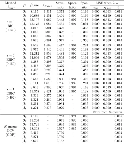
β1 7.196 – 0.753 0.971 0.000 0.008 β2 11.236 – 0.671 0.983 0.000 0.009 β3 13.721 – 0.639 0.984 0.000 0.011 β4 18.308 – 0.527 0.985 0.000 0.014 β5 6.415 – 0.759 – 0.000 0.004 β6 5.271 – 0.769 – 0.000 0.004 β7 5.629 – 0.767 – 0.000 0.004 β8 5.080 – 0.794 – 0.000 0.004 Table 2: Result of simulation experiment 2 under the linear model. Scaling weight parameter is set ats= 0 ands= 1. Tuning parameters are reported in log scale, i.e., ˜λ= log10(λ+ 1). Sparsity denotes the proportion of zero in estimation. Results are summarized from 1,000 replications.
Table 2 summarizes the simulation results for linear model where the errors are generated independently from N(0,1). Similar to simulation 1, FLARCC gives the smallest MSE for heterogeneous covariates, β1 toβ4, among all three models, and has comparable MSE as the homogeneous model for homogeneous covariates,β5 toβ8. More interestingly, whenK is large, BIC does not provide satisfactory model selection, erring on the lack of parsimony, while EBIC encourages stronger fusion and improves the ability to detect equal coefficient pairs in all eight covariates, regardless of their levels of heterogeneity. In addition, EBIC improves the sparsity detection among both the important and nonimportant covariates. It is interesting to note that the choice between BIC and EBIC does not alter solution paths, but only model selection. FLARCC with scaling weight parameter s = 1 has the best clustering performance among all compared methods. The difference between the choices of s= 0 ands= 1 is substantial in simulation 2, in contrast to the results from simulation 1. This indicates that the covariate-specific weights for heterogeneity {νj}pj=1 are very effective to improve the performance of the proposed fusion learning, especially when K
and p are large. Sensitivity and specificity of the two-stepK-means clustering method are higher than those of FLARCC with s= 0, but lower than those of FLARCC with s= 1. The two-step K-means has larger MSE than FLARCC because it does not consider the correlation between covariates. More importantly, the K-means clustering is a model-free method, so the results obtained from this method cannot be plugged in back to the model for prediction. As suggested from the empirical results of both simulation experiments, EBIC tends to provide better model selection for FLARCC than the conventional BIC.
6. Application: Clustering of Cohort Effects
In this data analysis example, we like to demonstrate the use of our method to derive clusters of cohort effects. Here we consider the Panel Study of Income Dynamics (PSID), which is a household survey study following thousands of families across different states in the US. PSID collects information of employment, income, health, and so on. In this data analysis, we focus on the association of household income with body mass index (BMI) on school-aged children between age of 11 and 19, adjusted for age, gender and birth weight. Data of 1880 children were gathered from four census regions (1-Northeast, 2-Midwest, 3-South and 4-West), as defined by U.S. Census Bureau (2015). All variables are standardized before model fitting. We are interested in investigating if regional heterogeneity exists and if the effects of interest differ across regions with region-dependent patterns.
Table 3 shows the results of coefficient estimates obtained from three different models: (A) homogeneous model (λ = λF use), coefficients estimated by combining data sets from four regions, (B) heterogeneous model (λ= 0), coefficients estimated separately by region-specific data, and (C) FLARCC (λ=λEBIC). Model A suggests that age and birth weight are positively associated with BMI for the subjects, but income was negatively associated with BMI. The estimates from Model B suggest that heterogeneous coefficient patterns exist among these associations since conclusions differ between regions. Model C appears more sensible when regression coefficients are heterogeneous across these regions. Since K
Region n Intercept Age Sex Birth Wt. Income
β0 β1 β2 β3 β4
(A) Homogeneous model – combine all regions
All regions 1880 0.000 0.206 0.016 0.063 -0.096 (B) Heterogeneous model – region specific estimates
1-Northeast 239 -0.133 0.228 -0.079 -0.003 0.004 2-Midwest 493 -0.054 0.229 0.017 0.124 -0.132 3-South 805 0.128 0.158 0.095 0.068 -0.071 4-West 343 -0.155 0.236 -0.083 0.057 -0.074
(C) Fused model using FLARCC
1-Northeast 239 -0.093 0.201 -0.036 0.000 0.000 2-Midwest 493 -0.093 0.201 0.000 0.021 -0.047 3-South 805 0.075 0.201 0.000 0.021 -0.047 4-West 343 -0.093 0.201 -0.036 0.021 -0.047
Table 3: Coefficient estimates of the homogeneous model (λ= λF use), the heterogeneous model (λ= 0) and the fused model using FLARCC withλselected by EBIC, respectively.
0.00 0.05 0.10 0.15 0.20 0.25 0.30
−0.1
0.0
0.1
0.2
Solution Path
log10(λ+1)
β
Intercept age sex birth_weight income
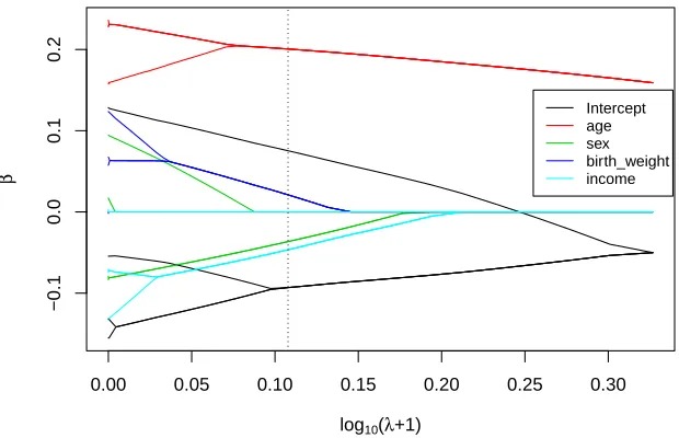
Figure 2: FLARCC solution paths of all covariates over the transformed tuning parameter ˜
Intercept_3 Intercept_2 Intercept_1 Intercept_4
0.00
0.10
0.20
0.30
Intercept
lo
g10
(
λ
+1)
Age_3 Age_4 Age_1 Age_2
0.00
0.02
0.04
0.06
0.08
Age
lo
g10
(
λ
+1)
Se
x_1
Se
x_4
Se
x_2
Se
x_3
0.00
0.05
0.10
0.15
0.20
Sex
lo
g10
(
λ
+1)
Bir
th_w
eight_1
Bir
th_w
eight_2
Bir
th_w
eight_3
Bir
th_w
eight_4
0.00
0.05
0.10
0.15
Birth_weight
lo
g10
(
λ
+1)
Income_1 Income_2 Income_3 Income_4
0.00
0.05
0.10
0.15
0.20
Income
lo
g10
(
λ
+1)
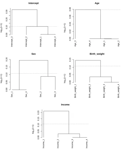
Based on the results from FLARCC, the estimated mean of standardized BMI in the South is 0.168 higher (or 0.97 higher in original scale of BMI) than that of the other three regions, which share the same mean. The effects of age are consistent across four regions. The effects of gender are classified into two clusters. The mean of standardized BMI of females is 0.036 lower (or 0.42 lower in original scale) than that of males in the Northeast and the West, but males and females have the same mean BMI in the Midwest and the South. Standardized BMI increases by 0.021 for every standard deviation increase of birth weight (or BMI increases by 0.19 for every unit increase of birth weight) in all regions except the Northeast. Similarly, standardized BMI decreases by 0.047 for every standard deviation increase of log income (or BMI decreases by 0.27 for every unit increase of income) in all regions except the Northeast where BMI is not affected by income. The leave-one-out mean squared prediction errors for model A, B and C are 0.953, 0.945 and 0.950, respectively. The differences between the prediction errors are small because of the relatively small effect sizes of the heterogeneous covariates identified by FLARCC, i.e., sex, birth weight and income. The most significant covariate, age, is homogeneous thus it does not differentiate the prediction power among the three models. Solution paths andfusograms of all covariates are shown in Figure 2 and Figure 3, respectively, for illustration. In summary, FLARCC ensures parsimony where necessary to maximize the prediction power of the final model; and it provides more informative interpretation and better visualization than the other two traditional models.
7. Concluding Remarks
The proposed method brings a new perspective to model fitting when combining multiple data sets from different sources is of primary interest. As data volumes and data sources grow fast, more and more opportunities and demands emerge in practice to borrow strengths of combined data sets. In such case, traditional methods are challenged by the complex data structures and do not provide desirable treatments and meaningful interpretations to data heterogeneity, especially when the number of data sets is very large. FLARCC allows the flexibility to explore the heterogeneity pattern of parameters among large number of data sets by tuning the shrinkage parameter.
When K and p are small, weights {νj}pj=1 do not contribute to much difference in terms of clustering and estimation. However, since only one tuning parameter is used to regularize the fusion of all covariates, when both K and p are large, we suggest letting
s > 0 to allow covariate-specific weights adapting to the heterogeneousness of coefficients
from individual covariates to achieve better results. In addition, the estimation consistency of rank estimator is a critical component needed to determine adjacent pairs. The current consistency is established under the case of K being fixed, and the validity of its property is unknown whenK increases along the total sample size.
Acknowledgments
We thank Drs. Fei Wang and Ling Zhou for helpful discussion. We are grateful to the action editor and two anonymous reviewers for their constructive comments that have led to an improvement of this paper. This research is supported by an NIH grant R01 ES024732.
Appendix A. Theorem Proofs
Proof of Theorem 1: The proof of Theorem 1 closely follows arguments given in Zou (2006). Without loss of generality, we assume n1 = · · · = nK = n and N = Kn. As K is fixed, n → ∞ implies N → ∞ in the same order. We assume the following regularity conditions:
(i) The Fisher information matrix is finite and positive definite,
I(θ∗) =Ehφ00X>θ∗XX>i.
Here, θ(Kp×1)∗ is the true parameters, X(N×Kp) is the design matrix corresponding toθ and φ is the link function (i.e., φ0 = h−1) defined in the following optimization problem
ˆ
θW = argmin θ
(
−1
K
K
X
k=1 1
nk
nk
X
i=1
Yk(i)Xk(i)>θ(λ)−φ
Xk(i)>θ(λ)
+Pλ,α(θ)
)
withPλ,α(θ) as defined in (4), and ˆθW is the estimator with true orderingW given.
(ii) There is a sufficiently large open setO that contains θ∗ such that∀θ ∈ O,
|φ000(X>θ)| ≤M(X>)<∞, and
E[M(X)|xjxkxl|]<∞
for a suitable functionM and all 1≤j, k, l≤Kp.
First we prove asymptotic normality. For ∀s≥0 and r >0, letθ=θ∗+u/√N. Define
ΓN(u) =− K
X
k=1 n
X
i=1
Yk(i)Xk(i)>
θ∗+√u N
−φ
Xk(i)>
θ∗+√u N
+λN p
X
j=1 K
X
k=1 ˆ
ωj,k
θ∗j,k+√uj,k
N
where ˆωj,k is specified in (6). Let ˆu(N) = arg minuΓN(u); then ˆu(N)=
√
N( ˆθW −θ∗). By Taylor expansion, we have ΓN(u)−ΓN(0) =H(N)(u), where
with
A(N)1 =−
K X k=1 n X i=1 h
Yk(i)−φ0(Xk(i)>θ∗)iX (i)> k u
√
N ,
A(N)2 =
K X k=1 n X i=1 1 2φ
00(X(i)> k θ
∗)u>X (i) k X
(i)> k
√
N u,
A(N)3 = √λN
N p X j=1 K X k=1 ˆ ωj,k √ N
θj,k∗ +√uj,k
N −
θj,k∗
,
andA(N)4 =N−3/2
K X k=1 n X i=1 1 6φ 000
Xk(i)>θ∗˜ Xk(i)>u
3 ,
where ˜θ∗ is between θ∗ and θ∗ +u/√N. The asymptotic limits of A(N)1 , A(N)2 and A(N)4
is exactly the same as those in the proof of Theorem 4 in Zou (2006). It suffice to show that A(N)3 has the same asymptotic limit. If θj,k∗ 6= 0, ˆωj,1 →p α|θ∗j,1|−r, ˆωj,k →p
|PK
k0=2θ∗j,k0|−s|θ∗j,k|−r for k = 2, . . . , K, and
√ N θ ∗ j,k+ uj,k √ N − θ ∗ j,k
→ uj,ksgn(θ∗j,k).
Thus by Slutsky’s theorem, A(N)3 → 0. If θj,k∗ = 0, for k = 1, since √Nθˆj,1 = Op(1), λN
√ NN
r−2α(|√Nθˆ
j,1|)−r → ∞; for k = 2, . . . , K, if PKk0=2θj,k∗ 0 = 0 (i.e., homogeneous),
√
NPK
k0=2θˆj,k0 =Op(1), thus √λN
NN
s+r
2 (| √
NPK
k0=2θˆj,k0|)−s(|
√
Nθˆj,k|)−r→ ∞; similarly, if
PK
k0=2θ∗j,k0 6= 0 (i.e., heterogeneous),
PK
k0=2θˆj,k0 →p PK
k0=2θ∗j,k0, √λN
Nωˆj,k → ∞ still holds. And since√N
θ ∗ j,k+ uj,k √ N − θ ∗ j,k
→ |uj,k|, we have the following result summary:
λN
√
Nωˆj,k
√ N
θ∗j,k+√uj,k
N −
θj,k∗ →p
0 ifθj,k∗ 6= 0
0 ifθj,k∗ = 0 and uj,k = 0
∞ ifθj,k∗ = 0 and uj,k 6= 0.
Following same arguments in Zou (2006)’s proof of Theorem 4, we have ˆu(N)A →dN(0,I11−1) and ˆu(N)Ac →d0. The proof of the consistency part is similar and thus omitted. Proof of Lemma 2: The estimated ordering ˆUjofβ∗j,
·
is only determined by the differences between distinct parameter groups within β∗j,·
. First note that for any 0 < < 1, if two parameters βj,k∗ and βj,k∗ 0 are in the same parameter group (i.e., β∗j,k = βj,k∗ 0), assigningwithout loss of generality, let βj,k∗ > β∗j,k0, the probability of estimating a wrong ordering
P1{βˆj,k0 ≥βˆj,k}>
=Pβˆj,k0 ≥βˆj,k
=P
ˆ
βj,k0−βˆj,k+β∗j,k−βj,k∗ 0 ≥β∗j,k−βj,k∗ 0
≤P|βˆj,k0 −β∗j,k0|+|βˆj,k−βj,k∗ |>0
= 1−Pβˆj,k0 =β∗
j,k0
Pβˆj,k =βj,k∗
→0
as n → ∞ since ˆβj,k0 and ˆβj,k are independent and consistent estimators. Similarly, the
consistency of the estimated ordering ˆVj of the absolute values in vectorβ∗j,
·
can be derived by taking the square of the absolute values and following the same argument as for ˆUj.Proof of Theorem 3: Here we assume the same regularity condition as in Theorem 1. To complete this proof, we first define the event W when the orderings of all p covariates are correctly assigned as
W =
p
\
j=1
{Ujˆ =Uj} ∩ {Vjˆ =Vj}.
Let ˆθWˆ be ˆθW when W occurs; otherwise, denote it as ˆθWc. Then, the estimator can be
rewritten as
ˆ
θWˆ = ˆθW1{W}+ ˆθWc1{Wc}
and therefore
√
NθˆWˆ −θ∗=√NθWˆ −θ∗1{W}+√NθWˆ c−θ∗
1{Wc}. (9)
By Theorem 1, we have √NθWˆ −θ∗ =O(1) and √NθWˆ c−θ∗
=O(1) as n → ∞.
By Lemma 2, we have P(W) → 1 and P(Wc) → 0 as n → ∞. Therefore, by Slutsky’s Theorem, (9) converge to the same distribution as √NθWˆ −θ∗. Similarly, by results from Theorem 1 and Lemma 2, we have selection consistency
P( ˆAWˆ =A) =P( ˆAWˆ =A|W)P(W) +P( ˆAWˆ =A|Wc)P(Wc)→1
asn→ ∞. This completes the proof of the Theorem 3.
Appendix B. Performance with Distorted Parameter Ordering
0 5 10 15 20
0.0
0.2
0.4
0.6
0.8
1.0
Percentage of wrongly ordered parameters
Sensitivity
β2
β3
0 5 10 15 20
0.0
0.2
0.4
0.6
0.8
1.0
Percentage of wrongly ordered parameters
Specificity
β2
β3
0 5 10 15 20
0.000
0.004
0.008
Percentage of wrongly ordered parameters
MSE
β2
β3
Figure 4: Clustering sensitivity and mean squared error of two heterogeneous slope param-eters β2 and β3 based on FLARCC with λselected by EBIC, as the percent of distorted ordering increases. Results are summarized from 100 replications.
parameters are displayed in Figure 4 for the two heterogeneous effects β2 and β3, and the homogeneous parameterβ1 is not included in the comparison because of no effect from the distortion on its performance. As the percentage of wrongly ordered parameters increases, as expected, sensitivity becomes lower and MSE becomes larger. However, specificity remains unaffected. When the distortion of ordering is mild (≤10%), the performance of FLARCC appears satisfactory in this simulation setting.
References
Jiahua Chen and Zehua Chen. Extended bayesian information criteria for model selection with large model spaces. Biometrika, 95(3):759–771, 2008.
Rebecca DerSimonian and Raghu Kacker. Random-effects model for meta-analysis of clinical trials: an update. Contemporary Clinical Trials, 28(2):105–114, 2007.
Jerome Friedman, Trevor Hastie, Holger H¨ofling, and Robert Tibshirani. Pathwise coordi-nate optimization. The Annals of Applied Statistics, 1(2):302–332, 2007.
Jerome Friedman, Trevor Hastie, and Robert Tibshirani. Regularization paths for gen-eralized linear models via coordinate descent. Journal of Statistical Software, 33(1):1, 2010.
Xin Gao and Peter X-K Song. Composite likelihood bayesian information criteria for model selection in high-dimensional data. Journal of the American Statistical Association, 105 (492):1531–1540, 2010.
Gene V Glass. Primary, secondary, and meta-analysis of research. Educational Researcher, 5(10):3–8, 1976.
Lars Peter Hansen. Large sample properties of generalized method of moments estimators. Econometrica, 50(4):1029–1054, 1982.
Zheng Tracy Ke, Jianqing Fan, and Yichao Wu. Homogeneity pursuit. Journal of the American Statistical Association, 110(509):175–194, 2015.
Jeffrey T Leek and John D Storey. Capturing heterogeneity in gene expression studies by surrogate variable analysis. PLoS Genetics, 3(9):1724–1735, 2007.
Hung-Mo Lin, H Myron Kauffman, Maureen A McBride, Darcy B Davies, John D Rosendale, Carol M Smith, Erick B Edwards, O Patrick Daily, James Kirklin, Charles F Shield, and Lawrence G Hunsicker. Center-specific graft and patient survival rates: 1997 united network for organ sharing (unos) report. Journal of the American Medical Asso-ciation, 280(13):1153–1160, 1998.
Dungang Liu, Regina Y Liu, and Minge Xie. Multivariate meta-analysis of heterogeneous studies using only summary statistics: efficiency and robustness. Journal of the American Statistical Association, 110(509):326–340, 2015.
Kirk E Lohmueller, Celeste L Pearce, Malcolm Pike, Eric S Lander, and Joel N Hirschhorn. Meta-analysis of genetic association studies supports a contribution of common variants to susceptibility to common disease. Nature Genetics, 33(2):177–182, 2003.
Thomas Lumley and Alastair Scott. AIC and BIC for modeling with complex survey data. Journal of Survey Statistics and Methodology, 3(1):1–18, 2015.
Wei Pan, Xiaotong Shen, and Binghui Liu. Cluster analysis: unsupervised learning via su-pervised learning with a non-convex penalty. The Journal of Machine Learning Research, 14(1):1865–1889, 2013.
Jin Qin and Jerry Lawless. Empirical likelihood and general estimating equations. The Annals of Statistics, 22(1):300–325, 1994.
Gideon Schwarz. Estimating the dimension of a model. The Annals of Statistics, 6(2): 461–464, 1978.
Paul G Shekelle, Mary L Hardy, Sally C Morton, Margaret Maglione, Walter A Mojica, Marika J Suttorp, Shannon L Rhodes, Lara Jungvig, and James Gagn´e. Efficacy and safety of ephedra and ephedrine for weight loss and athletic performance: a meta-analysis. Journal of the American Medical Association, 289(12):1537–1545, 2003.
Xiaotong Shen and Hsin-Cheng Huang. Grouping pursuit through a regularization solution surface. Journal of the American Statistical Association, 105(490):727–739, 2010.
Sunyoung Shin, Jason Fine, and Yufeng Liu. Adaptive estimation with partially overlapping models. Statistica Sinica, 26(1):235–253, 2016.
Alexander J Sutton and Julian Higgins. Recent developments in meta-analysis. Statistics in Medicine, 27(5):625–650, 2008.
Robert Tibshirani. Regression shrinkage and selection via the lasso. Journal of the Royal Statistical Society: Series B (Statistical Methodology), 58(1):267–288, 1996.
Robert Tibshirani, Michael Saunders, Saharon Rosset, Ji Zhu, and Keith Knight. Sparsity and smoothness via the fused lasso. Journal of the Royal Statistical Society: Series B (Statistical Methodology), 67(1):91–108, 2005.
U.S. Census Bureau. Regions and divisions.http://www.census.gov/econ/census/help/ geography/regions_and_divisions.html, 2015. [Online; accessed 10-31-2015].
Fei Wang, Lu Wang, and Peter X-K Song. Fused lasso with the adaptation of parameter ordering in combining multiple studies with repeated measurements. Biometrics, 2016. doi: 10.1111/biom.12496. Advance online publication.
Minge Xie, Kesar Singh, and William E Strawderman. Confidence distributions and a unifying framework for meta-analysis. Journal of the American Statistical Association, 106(493):320–333, 2012.
Sen Yang, Lei Yuan, Ying-Cheng Lai, Xiaotong Shen, Peter Wonka, and Jieping Ye. Fea-ture grouping and selection over an undirected graph. In Proceedings of the 18th ACM SIGKDD international conference on Knowledge discovery and data mining, pages 922– 930. ACM, 2012.
Jianming Ye. On measuring and correcting the effects of data mining and model selection. Journal of the American Statistical Association, 93(441):120–131, 1998.