A Point Memory State Observer with Adjustable Parameters for a Class of Uncertain Linear Systems with State Delays

(1)

A Point Memory State Observer with Adjustable Parameters for a Class

of Uncertain Linear Systems with State Delays

Shunya Nagai

1

, Hidetoshi Oya

2,*

, and Tsuyoshi Matsuki

3

1_{Department of Information Systems Creation, Kanagawa University, Kanagawa, Japan} 2_{Department of Computer Science, Tokyo City University, Tokyo, Japan}

3_{Department of Electronics and Control Engineering, National Institute of Technology, Niihama College, Ehime, Japan} Received 10 May 2018; received in revised form 26 November 2018; accepted 07 December 2018

Abstract

In this paper, we present a point memory robust state observer with time-varying adjustable parameters for a class of uncertain linear systems with state delays. The point memory robust state observer proposed in this paper consists of fixed observer gain matrices and time-varying adjustable parameters, which are determined by updating rules. Sufficient conditions for the existence of the proposed point memory robust state observer can be reduced to solvability of LMIs. Finally, simple numerical examples are included to illustrate the effectiveness of the proposed robust state observer.

Keywords: point memory robust state observer, time-varying adjustable parameters, state delays, LMIs

1. Introduction

Time delays are a phenomenon that occurs in physical systems such as manufacturing, long transmission lines in networked control systems and so on. When designing control systems, time delays is usually the reason that generates oscillation, poor performance, or instability of underlying control systems. Namely, dealing with time delays is an important issue of controller design, and designers have to manage time delays so as to avoid the negative effects on the performance of control systems. Therefore, various control strategies for time-delay systems have been widely studied (see. [1] and references therein). In particular, [2] has adopted a point memory feedback strategy and presented an LMI-based design method of LQ regulator for a class of time-delay systems. Additionally, for uncertain time delay systems, lots of existing results for robust controller design methods have been shown (e.g. [3-4]). Particularly, in the work of [5], a guaranteed cost controller for a class of uncertain time-delay systems has been suggested. Furthermore, a variable gain robust controller for a class of uncertain linear systems with state delays has also been proposed [6].

By the way, in the control theory, the concept of state variable feedback is the most fundamental strategy for controlling dynamical systems. In particular, for linear systems, when the liner system is controllable (e.g. [7-8]) and references therein), the closed-loop poles arbitrary can be assigned. However, due to physical, technical and/or economic reasons, not all variables can be measured; designers have to be able to deduce information on the state of the dynamical system by means of observations and measurements or a priori knowledge of the system structure. Namely, the so-called state observers must be designed. If the estimate of the state variable can be constructed, by using the estimate can derive from a feedback control system based on the state observer. It is well-known that the state observer was first presented and developed by [9-10], and further studied by many researchers (e.g. [11]). The observer design only aimed to linear time-invariant systems with complete

(2)

knowledge of system parameters, also the input and output signals. However, it is inevitable to include uncertain parameters and parameter variations; at the same time, the controlled systems are affected by unknown disturbances. Therefore, state observers which guarantee the exactness of state estimation in the presence of unknown parameters are required. Thus, the design problem of robust state observers for uncertain dynamical systems has been well studied, and in order to deal with this problem, a large number of existing results of robust state observer design have been presented [12-13]. In the work of Wang et al.[14], a design method of an optimal observer of uncertain linear systems has been proposed. Note that these robust state observers have fixed observer gains. Furthermore, a robust state observer for linear systems with perturbations has been shown [15]. The [15] have introduced time-varying complementary variables, and based on a Riccati equation approach a design method of the robust state observer has been suggested. Additionally, the relation between solvability of the derived Riccati equation and H∞-norm performance of a transfer function has been analyzed. For their work, a comment and authors' reply have also been presented [16-17]. However, the robust state observer given in [15] is incomplete.

In this paper, on the basis of the existing result [6], we present a point memory robust state observer with time-varying adjustable parameters for a class of uncertain linear systems. The proposed point memory robust state observer consists of a time-varying adjustable parameter and a number of fixed gain parameters. In this paper, we derive complete sufficient conditions of the existence of the proposed variable gain robust state observer, and the sufficient conditions are given in terms of LMIs. This paper is organized as follows; Notations and useful lemmas, which are used in this paper, are shown in Section 2. In Section 3, we show the class of uncertain linear systems under consideration and an observer with fixed and time-varying adjustable parameters. Section 4 is the main result in this paper. The design method of the proposed point memory robust state observer with time-varying adjustable parameters is presented. Finally, we show simple illustrative examples to show the effectiveness of the robust state observer developed in this paper.

2. Preliminaries

In this section, notations, well-known and useful lemmas (see [18] for details) which are used in this paper are presented. The following notations are used in this paper. For a matrix ,S the inverse of matrix ,S and its transpose are denoted by 1

,

S andS,T, respectively. Moreover, H_e

 

S and

I

_n mean SST and

n

-dimensional identity matrix, respectively, and for real symmetric matrices W and Z, W Z (resp. W Z) means that W Zis positive (resp. nonnegative) definite matrix. For a vector

w





n

,

w denotes standard Euclidian norm and for a matrix W, W represents its induced norm. The symbols “



” and “



” mean equality by definition and symmetric blocks in matrix inequalities, respectively.

Lemma 1 (Schur complement formula [18]) : For a given constant real symmetric matrix , the following items are equivalent:

(i) ψ = (ψ_∗11 ψ_ψ12

22) > 0,

(ii) ψ₁₁> 0 and ψ₂₂− ψ₁₂T ψ₁₁−1ψ₁₂> 0, (iii) ψ22> 0 and ψ11− ψ12ψ22−1ψ12T > 0.

3. Problem Formulation

Consider the uncertain time delay system described as the following state equation;









), ( ) (

), ( ) ( ) ( )

( ) ( )

( t Cx t y

t Bu h t x E t C A t x E t C A t x dt d

h h T h T



  

  

 

(1)

(3)

n q

E  and E_h qhn denote the structure of unknown parameters. Moreover (t)lq and _h(t)lqhare unknown time-varying parameters which satisfy the relations | |(t)| |1.0 and | |_h(t)| |1.0, respectively.

Now the design problem under consideration is how to design a variable gain robust state observer with the measured output y(t)l and the control input u(t)m. The estimation error between the state variable and the estimate based on the observer can converge asymptotically to 0. In this paper, we introduce the following point memory robust state observer;

), ( ) ( )) ( ) ( ( )) ( ) ( ( ) ( ) ( )

( y t h Cx t h Bu t t

h L t x C t y L h t x h A t x A t x dt d



                (2)

wherex t n 

)

( is the estimate of the state variable x(t), and Lnl and L_h nl are fixed observer gain parameters. Moreover (t)n in Eq. (2) is a compensation input with time-varying adjustable parameters [6]. Then we obtain the following estimation error system;

),

(

)

(

)

(

)

(

)

(

)

(

)

(

)

(

)

(

)

(

t

A

LC

e

t

A

_h

L

_h

C

e

t

h

C

T

t

Ex

t

C

T

_h

t

E

_h

x

t

h

t

e

dt

d





















(3)

where e(t) is an estimation error vector defined as e(t) x(t) x(t)  

 ,

From the above, our control objective in this paper is to construct the point memory robust state observer of Eq. (2), for the uncertain time-delay system of Eq. (1). That is to derive the fixed gain matrices Lnl and L_h nl, and the compensation input



(t)n such that the estimation error system of Eq. (3) is asymptotically stable.

4. Main Results

In this section, we derive an LMI-based design procedure for the proposed point memory robust state observer with time-varying adjustable parameters. Next theorem gives a sufficient condition for the existence of the proposed robust state observer.

Theorem 1: Consider the uncertain time delay system of Eq. (1) and the robust state observer of Eq. (2).

If the symmetric positive matrices exist, Pnn , P_hnn and Xll, matrices Wnl and W_h nl and positive scalars 

,

_h

,



and _h which satisfy the LMIs





,

0

0 











































l

I

h

l

I

h

l

I

l

I

l

n

l

n

l

n

l

n

h

E

T

h

E

h

P

T

PC

T

PC

T

PC

T

PC

C

h

W

h

PA

h

P

E

T

E

WC

P

T

A

e

H









(4) , 0  



_









l I T PC XC T C (5)

then the fixed gain matrices Lnl and L_hnl are determined as LP1W and L_h P1W_h, respectively and the compensation input



(t)n is designed as:

(4)

Proof: In order to prove Theorem 1, we introduce the following function:

.

) ( 1 2 ) ( 2 / 1 2 ) ( 2 ) ( )

( P CTXCe t

t Ce X h t x h E h t x E t          (6)

By using the point memory robust state observer with the fixed gain matrices Lnl and L_hnl , and the compensation input (t)n , the estimation error e(t)converges asymptotically to 0.

.

0 ) ( ) ( ) ( ) ( ) , (       h d t e h P t T e t Pe t T e t e

V



(7)

The time derivative of the function V(e,t)of Eq. (7) along with the trajectory of the estimation error system of Eq. (4) is given by





( , ) ( ) ( ) ( ) 2 ( ) ( ) ( )

2 ( ) ( ) ( ) 2 ( ) ( ) ( )

2 ( ) ( ) ( ) ( ) ( ) ( ).

d _T _T _T

V e t e t H_e P A LC e t e t PC t Ex t dt

T T T

e t P A_h L C e t_h h e t PC _h t E x t_h h

T T T

e t P t e t P e t_h e t h P e t_h h

 

 _  _  

     

    

(8)

If the relation eT(t)PCTCPe(t)0 holds, then it is to be seen from Eq. (6) and the relation 2eT(t)P(t)0that the following inequality is satisfied;





( , )

( )

(

)

( ) 2

( ) (

) (

)

( )

(

)

(

)

d

_T

V e t

e

t

H

P A LC

e t

e

t P A

L C e t

h

e

h

dt

T

e

t P e t

e

t

h P e t

h







_



_









(9)

The inequality of Eq. (9) can be written as:





.

) ( ) ( ) ( ) ( ) ( ) ( ) , (





































        h t e t e h P C h L h A P h P LC A P e H T h t e t e t e V dt d (10)

Thus the matrix inequality:





, 0 ) ( ) (      













h P C h L h A P h P LC A P e H (11)

is satisfied, then the following relation holds;

( , )

0,

( )

0 (

)

0. d

V e t

e t

and

e t

h

dt













(12)

Next we consider the case of eT(t)PCTCPe(t)0. Additionally, we introduce the relation:

), ( ) ( ) ( )

(t PCTCPet eT t CTXCet T

e  (13)

where Xll is a symmetric positive definite matrix. Note that if the condition eT(t)CTXCe(t)0 holds then 0

) ( )

(t PC CPet 

eT T is also satisfied.

(5)

, CP T PC XC T

C  (14)

By applying Lemma 1(Schur complement formula) to Eq. (14), we obtain

. 0   _     l I T PC XC T C (15)

It is obvious that if the condition of Eq. (10) holds, then we have eT(t)CTXCe(t)0in the case of eT(t)PCTCPe(t)0.

From the definition of the estimation error vector, the relations

x

(

t

)

e

(

t

)

x

(

t

)







and x(t h) e(t h) x(th)    

 holds.

Therefore, the time derivative of the function V(e,t)can be rewritten as









( , ) ( ) ( ) ( ) 2 ( ) ( ) ( ( )) ( ))

2 ( ) ( ) ( ) 2 ( ) ( ) ( ( ) ( )) 2 ( ) ( ) ( ) ( ) ( ) ( )

( ) ( ) ( ) 2 ( ) ( C) ( )

d _T _T _T

V e t e t H P A LC e t e t PC t E e t x t

e dt

T T T

e t P A L C e t h e t PC t E e t h x t h

h h h h

T T T

e t P t e t P e t e t h P e t h

h h

T T

e t H P A LC e t e t P A L e t

e h h h

     _  _                     _  _  

1 ( ) ( ) ( ) ( )

1 ( ) ( ) ( ) ( ) 1 ( ) ( ) ( ) ( ) 1 ( ) ( ) ( ) ( )

2 ( ) ( ) ( ) ( ) ( ) ( ).

T T T T

e t PC CPe t e t E Ee t

T

T T T

e t PC CPe t x t E E x t

T T T T

e t PC CPe t e t h E E e t h

h h

h

T

T T T

e t PC CPe t h x t h E E x t h

h h

h

T _{t P t} _eT _{t P e t} _eT _t _{h P e t} _h

h h                              (16)

Here we used the relation e(t) x(t) x(t)  

 and the well-known inequality

b T b a T a b T a   1

2   (17)

for any vectors

a

and b with appropriate dimensions and any positive constant . By substituting the compensation input of Eq. (6) to Eq. (16) and some algebraic manipulations gives

.

) ( ) ( ) , , , , , ( ) ( ) ( ) , (

























    h t e t e h h h P P T h t e t e t e V dt d     (18)

In Eq. (15), (P,P_h,_h,,,_h)2n2nis the matrix given by













      h P C h L h A P h h h P P h h h P

P, , , , , ) 11( . , , , , ) ( )

(









(19)





PCTCP ETE P_h

h h LC A P e H h h h P

P        



_























, , , ) ( ) 1 1 1 1

, , (

11 (20)

Therefore, the inequality condition of Eq.(12) is satisfied provided that the following condition holds,

. 0 ) , , , , , ( 

(6)

Additionally, one can clearly see that the matrix inequality of Eq. (21) is a sufficient condition of Eq. (11), i.e. if the matrix inequality of Eq. (21) holds then the condition of Eq. (11) is also satisfied.

Finally, we consider the matrix inequality of Eq. (21). By applying Lemma 1 (Schur complement formula) to Eq. (21), we can obtain the LMI of Eq. (4). Thus, the proof of Theorem 1 is accomplished.

5. Numerical Example

This section shows a simple numerical example to demonstrate the proposed point memory robust state observer. In this example, we consider the uncertain time delay system given by





1.0 1.0 1.0 0.5 0.0

( ) ( ) ( )

0.0 1.0 1.0 0.0 0.0

0.5 0.0 1.0 0.0 0.0 0.0

( ) ( 0.5) ( ),

0.0 0.5 1.0 0.0 0.5 1.0

( ) 1.0 1.0 ( ).

h

d

x t t x t

dt

t x t u t

y t x t

      

 

 _     

     

 

       

 

__ _{ } _ _ __  _ _

       

 



　　　 (22)

Firstly, by solving LMIs of Eq. (4) and Eq. (5), we have symmetric positive definite matricesP2 2 , 2 2 h

P  and 1 1

X , matrices W2 1 and W_h2 1 and positive scalars 

,

_h

,



and _h as

3 2

3

3 3 2

2 2 2

2.1570 2.1208 _{5.6711 10} _{1.3509 10}

10 , ,

6.4073 10 2.1570

4.2335 5.0857

4.0718 10 , 10 , 10 ,

1.7941 4.9957

5.4931 10 , 5.4351 10 , 5.4737 10 , 5.4632 10

h

h h

P P

X W W

   



      

_ _  



 



   

  _ _ _ _

   

      



　　 = 　 2

.

(23)

Thus the fixed gain matrices L2 1 and 2 1 h

L  can be calculated as

1 1

3

8.3413 2.4208 10

10 , .

8.2843 h 6.4078 10

L L



  

 

   _ _ 

  　   (24)

In this example, initial values for the uncertain linear system of Eq. (22) and the proposed variable gain robust state observer are selected as x(0) 



1.0 0.5



T and



x

(0)



0.0 0.0



T, respectively. Furthermore, unknown parameters are given as





( )t 0.0 cos(5 )t

  and, respectively. Moreover, we assume that the control input is given by u t( )sin( )t .

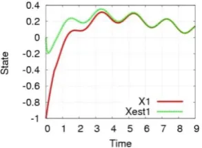
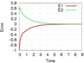
The simulation result of this numerical example is shown in Figs. 1-4. In these figures, Xl, Xextl and El (l=1,2) denotes the l-th element of the state, the estimate of the state variable and the estimation error. From these figures, we can see that the proposed point memory robust state observer can estimate the state variables of the uncertain time delay system of Eq. (22) and the estimation error for the proposed point memory robust state observer converges to 0. Thus we have shown the effectiveness of the proposed point memory robust state observer.

(7)

Fig. 3 Time histories of the first e t( ) Fig. 4 Time histories of e t( )

6. Conclusions

In this paper, on the basis of the work of Endo et al.[6], we have proposed a new point memory robust state observer for a class of uncertain time delay systems. The sufficient condition for the existence of the proposed point memory robust state observer is reduced to LMIs, and thus the proposed robust state observer can easily be obtained.

Future research subjects are going to extend the proposed point memory robust state observer to uncertain large-scale interconnected systems with state delays, uncertain discrete-time systems and so on. Furthermore, we will evaluate the conservativeness of the proposed observer design.

Conflicts of Interest

The authors declare no conflict of interest.

References

[1] K. Gu, V. L. Kharitonov, and J. Chen, “Stability of time-delay systems,”Birkhauser, 2003.

[2] T. Kubo, “LQ regulator of systems with time-delay in the states by the point memory feedback,” IEICE Trans. Fundamentals of Electronics, Communications and Computer Sciences, vol. J87-A, no. 4, pp. 577-579, 2004.

[3] X. Li and C. E. D. Souza, “Delay-dependent robust stability and stabilization of uncertain linear delay systems: a linear matrix inequality approach,” IEEE Transactions on Automatic Control, vol. 42, no. 8, pp. 1144-1148, August 1997. [4] X. Li and C. E. D. Souza, “Criteria for robust stability and stabilization of uncertain linear systems with state delay,”

Automatica, vol. 33, no. 9, pp. 1657-1662, September 1997.

[5] L. Yu and J. Chu, “An LMI approach to guaranteed cost control of linear uncertain time delay systems,” Automatica, vol. 35, no. 6, pp. 1155-1159, June 1999.

[6] K. Endo, H. Oya, T. Kubo, and T. Matsuki, “Synthesis of variable gain robust controllers based on point memory LQ regulator for a class of uncertain time-delay systems,” 2015 10th Asian Control Conference, IEEE Press, pp. 2957-2961, September 2015.

[7] M. Norton, “Modern control engineering,” Pergamon Press, 1972.

[8] B. D. O. Anderson and J. B. Moore, “Optimal control-linear quadratic method,” Prentice Hall, 1990.

[9] D. G. Luenberger, “Observing the state of a linear system,” IEEE Transactions on Military Electronics, vol. 8, no. 2, pp. 74-80, 1964.

[10] D. G. Luenberger, “Observer for multivariable systems,” IEEE Transactions on Automatic Control, vol. 11, no. 2, pp. 190-197, April 1966.

[11] B. Gopinath, “On the control of linear multiple input-output systems,” The Bell System Technical Journal, vol. 50, no. 3, pp. 1063-1081, 1971.

[12] J. C. Doyle and G. Stein, “Robustness with observers,” IEEE Transactions on Automatic Control, vol. 24, no. 4, pp. 607-611, 1979.

[13] B. L. Walcott and S. H. Zak, “Observation of dynamical systems in the presence of bounded nonlinearities/uncertainties,” 25th IEEE Conference on Decision and Control, IEEE Press, April 2007.

(8)

[15] D. W. Gu and F. W. Poon, “A robust state observer scheme,” IEEE Transactions on Automatic Control, vol. 46, no. 12, pp. 1958-1963, December 2001.

[16] M. Boutayab and M. Darouach, “Comments of a robust state observer scheme,” IEEE Transactions on Automatic Control, vol. 48, no. 7, pp. 1292-1293, 2003.

[17] D. W. Gu and F. W. Poon, “Authors’ reply,” IEEE Transactions on Automatic Control, vol. 48, no. 7, p. 1293, 2003. [18] S. Boyd, L. E. Ghaoui, E. Feron, and V. Balakrishnan, “Linear matrix inequalities in system and control theory,” SIAM,

1994.

[19] M. Maki and K. Hagino, “Robust control with adaptation mechanism for improving transient behaviour,” International Journal of Control, vol. 72, no. 13, pp. 1218-1226, 1999.