155
Copyright © 2011-15. Vandana Publications. All Rights Reserved.
Volume-5, Issue-2, April-2015
International Journal of Engineering and Management Research
Page Number: 155-161
A Baseline Framework Model for an Emission-free Fuel Cell Vehicle
System employing Highway and Federal Driving Procedure
M.Karthik1, S.Usha2, S.Sreemathy3
1,2
Department of Electrical and Electronics Engineering, Kongu Engineering College, Perundurai, Erode, INDIA
3
Department of Electronics and Instrumentation Engineering, Kongu Engineering College, Perundurai, Erode, INDIA
ABSTRACT
In this paper the performance of Neural Network (NN) based fuel cell powered electric vehicle model is analyzed for three different modified drive cycle patterns such as M-HWY, M-US06 and M-FTP based on which they are operated. The complexity involved in the conventional mathematical modeling of the fuel cell stack system is eradicated with the Neural Network modeling. The Multilayer feed forward Neural Network is used to predict the output voltage of the PEM fuel cell from a predefined vehicle drive cycle pattern. The optimum neural network is chosen by varying the training algorithms and the number of neurons in the hidden layer. The performance comparison in terms of error minimization values such as MSE, MAE and iteration value is also carried out to verify the reliability of the optimum neural network. The optimum neural network chosen is used to develop a neural network based fuel cell driven electric vehicle model that includes the modeling of fuel cell, DC-DC converter and vehicle dynamics. The simulation results obtained from the developed electric vehicle model are used to evaluate the vehicle performance in terms of hydrogen consumption, maximum distance coverage and power flow within the vehicle system. The comparison of the required vehicle power with the fuel cell (Neural Network) delivered power is carried out to validate the optimality of the proposed electric vehicle model.
Keywords— Driving procedure, Emission-free vehicle Fuel Cell, DC-DC converter, Multi-Layer Perceptron Neural Network, Vehicle dynamics
I.
INTRODUCTION
Environmental, political, and monetary drivers have aligned on the need for sustainable transportation, requiring a long-term transition to fossil-free energy vectors. This transition will be evolutionary with many
experts predicting a continual increase in the electrification vehicles. Also the statistical analysis reports that the world oil reserve will be depleted by the year 2049 [6]. Increasing energy consumption in the world, rise in emissions and the depletion of fossil fuels are the justifiable reasons for using electrical vehicles (EVs) instead of fossil-fuel vehicles. Among the several sectors, the vehicle sector is the most promising and emerging one which utilizes the fossil fuel to a greater extent that leads to air pollution and global warming. The EVs are proposed as an attractive solution for the transportation applications that provide environmentally friendly operation with the usage of clean and renewable energy sources. Among all other energy sources, Fuel Cell is one of the most promising candidates for fuel-efficient and emission-free vehicle propulsive power.
156
Copyright © 2011-15. Vandana Publications. All Rights Reserved.
In this paper, Artificial Neural Network technique is used to predict the stack voltage of PEM fuel cell. This paper is also focused on the design, modeling and simulation of the artificial neural network based fuel cell powered vehicle model and the performance of the proposed electric vehicle model is also analyzed based on the three different modified drive cycle patterns (M-US06/M-HWY/M-FTP) based on which they are operated.
II.
EMISSION FREE VEHICLE
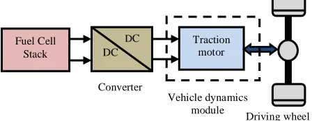
The fundamental components involved in the development of the electric vehicles are the fuel cell stack system, unidirectional converter and the vehicle dynamics. All the components involved in the proposed model are developed individually and incorporated to form a Fuel Cell Electric Vehicle. The complete model of the proposed electric vehicle is shown in Fig. 1. Initially the standalone fuel cell driven electric vehicle modeling is started with the development of the fuel cell stack model that includes fuel cell stack sizing and polarization dynamics. A single fuel cell is not capable to offer the nominal power required to meet the load demand. Hence the necessary number of fuel cells is connected in series to form fuel cell stack that yield nominal voltage and power in order to propel the electric vehicle. The output of the fuel cell stack can be unregulated output voltage which cannot be connected directly with the vehicle dynamics module since the vehicle dynamics module requires always constant power for propulsion. Hence there is a need for the converter circuitry for converting the unregulated output voltage into regulated one. The regulated output voltage from the converter unit propagates towards the vehicle dynamics module to provide power to the wheel [2].
Figure 1: Proposed Electric Vehicle Model Framework
PEM FUEL CELL MODELING
PEM fuel cell is mostly used in automotive applications because of its attractive features. The behavior of the PEM fuel cell stack system is highly affected by the various polarization losses and also various electrochemical, thermodynamic and thermal processes takes place inside the fuel cell stack system which makes that system to behave as a highly non-linear. The PEM fuel cell parameters are time varying and it is very difficult to keep them unchanged during its operation. Hence it is very
difficult to perform mathematical modeling. Hence some other intelligent techniques have to be used to overcome the complexity in conventional modeling. One such technique is neural network approach [4]. The neural network approach does not require any prior knowledge of processing parameters. The neural network approach is required to indicate a better control performance with appropriate input and output parameter selection. From the polarization dynamics of the fuel cell, the selection of input and output parameters depends on the effect of operating current, anode and cathode operating pressure, hydrogen and oxygen fuel consumption on cell performance.
The input parameters chosen for modeling the neural network are current density, partial pressure of hydrogen and oxygen and the outputs from the network are stack voltage, stack power and hydrogen consumption and the neural network with the defined inputs and outputs is shown in Fig. 2.
Figure 2: Input-Output Parameter Set
TABLEI
Fuel cell specifications
The specifications of the proposed fuel cell stack system are given in Table 1. The data required to train the network is generated from the simulation model of Ballard 5KW PEM fuel cell developed in MATLAB/SIMULINK environment [1].
CONVERTER MODELING
The output of the fuel cell stack system is non linear due to incidence of electrochemical reaction inside the fuel cell. Hence there is a need of power electronic circuitry to stabilize the nonlinear output from the fuel cell stack system. Therefore DC-DC converter circuit is developed for converting the unregulated output voltage into regulated output voltage [3]. The converter employed along with the fuel cell is unidirectional DC-DC converter since it does not have the capability to make use of the power developed from the wheels of the vehicle during braking.
S.No. Parameters Specifications
1 Number of fuel cells in stack 35 2 Maximum power output(kW) 5 3 Nominal cell voltage(V) 0.5-1.2 4 Nominal stack voltage(V) 17.5-42 5 Type of fuel cell PEM
Driving wheel Vehicle dynamics
module Converter
Traction motor Fuel Cell
Stack DC DC
V P NHx
cH2 I
pH2 pO2
157
Copyright © 2011-15. Vandana Publications. All Rights Reserved.
The output voltage (Vout) of the proposed DC-DC
converter in terms of input voltage (Vin
D) -(1
in V = out V
) and duty ratio (D) is shown as in Eq. 1,
Duty ratio in terms of reference voltage and converter output voltage is given as in Eq. 2,
(
Vout Vref)
dtD=∫ −
The output current (Iout) of the proposed DC-DC
converter in terms of input current (Iin
D) -η(1
in I = out I
), efficiency (η) and duty ratio (D) is given as in Eq. 3,
VEHICLE DYNAMICS MODELING
In this paper, the vehicle model is developed for the low power vehicle driven applications. The vehicle dynamics modeling is designed in apprehension with the total resistive force or tractive force acting on the vehicle and power required to drive the vehicle.
The motor output power (PM) is the function of
velocity (Va) and total resistive force (Ft
a V × t F = M P
) and it is shown as in Eq. 4,
The tractive force (Ft)acting on the driving wheel
is the sum of four different forces and it is represented as in Eq. 5
grade F + if F + rr F + ad F = t F
,
where,
Fad- Aerodynamic drag force (N)
Frr- Rolling resistance force (N)
Fif- Inertial force (N)
Fgrade- Grade force (N)
The electrical power (PE) required for running the
motor is the function of mechanical power (PM
η M P = E P
) and efficiency (η) which is given as in Eq. 6,
The vehicle parameters specifications for our proposed electric vehicle model are taken from the paper [7] and it is listed in Table 2.
III.
DEVELOPMENT OF MLP
NETWORK
The Multi Layer Perceptron (MLP) Network is one of the static feed forward networks based on the error back propagated to the multi-layer model network that provide non-linear mapping between input and output parameters [5].
The architecture of the feed forward MLP network is shown in Fig. 3. The MLP network shown consists of three layers namely input, hidden and output layer. Network with single hidden layer is used in this paper, in order to reduce the network complexity.
(1)
(3)
(4) (2)
(5)
158
Copyright © 2011-15. Vandana Publications. All Rights Reserved.
The net input to the hidden layer is the function of input, weights and bias and it is as shown as in Eq. 7,
j θ n
0
i Xi Wij (X)
Gj ∑ +
= ×
=
(
)
Since the input range is normalized in between [-1, 1], hence the activation function performed on the input signal is hyperbolic tangential sigmoidal (tansig) and it is shown as in Eq. 8,
(X) j G e (X) j G e
(X) j G e (X) j G e (X)) j tanh(G (X) j Y
− +
− − =
=
The results from the hidden layer is propagates towards the next layer. The net input to the output layer is represented as in Eq. 9,
k θ n
0
j Yj(X) Vjk (X)
k
G ∑ +
= ×
=
(
)
In order to provide linear output signal, the linear output function is performed at the output layer and it is expressed as in Eq. 10,
(X) k G = k Y
The prediction performance of the proposed MLP network in terms of performance indices such as Mean Square Error (MSE), Mean Absolute Error (MAE), Mean Absolute Percentage Error (MAPE), Regression Analysis and Iteration Value by varying the training algorithm and number of neurons in the hidden layer is analyzed [5]. Results obtained for four different training algorithms (such as trainlm, trainrp, trainscg and trainbfg) and varying the hidden neurons from 1 to 15.
Table 3 shows the training results obtained for trainlm training algorithm using MLP Network with the number of neurons 10 in the hidden layer. From Table 3, it can be concluded that, the optimum training algorithm is Levenberg-Marquardt (trainlm) algorithm and the optimum neurons for the hidden layer is 10 and it yields good prediction performance with minimum MSE value of 1.0588e-05 within 8 epochs and the response of the MLP network is shown in Fig 4.
0 2 4 6 8
10-5
100
Best Validation Performance is 1.0588e-05 at epoch 8
Me
an
S
q
u
ar
ed
E
rr
or
(
m
se
)
8 Epochs
Figure 4: MLP Network Response
IV.
RESULTS AND DISCUSSION
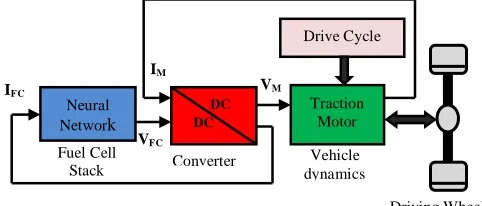
In this section, simulation results of the proposed neural network based fuel cell driven electric vehicle are discussed. The simulation work is carried out using MATLAB/Simulink environment to verify the reliability of the electric vehicle model performance by applying a three different modified drive cycle patterns as a input and the performance characteristics of the proposed electric vehicle model are also investigated. The block diagram representation of the neural network based fuel cell powered electric vehicle model which is implemented in the MATLAB/Simulink is shown in the Fig. 5.
Figure 5: MATLAB Implementation of Proposed Electric Vehicle Model
M-US06 DRIVING CYCLE
A driving cycle commonly represents a set of vehicle speed points versus time. It is used to assess fuel consumption and pollutants emissions of a vehicle in a normalized way, so that different vehicles can be compared. The driving cycle is performed on a chassis dynamometer, where tailpipes emissions of the vehicle are collected and analyzed to assess the emissions rates.
The M-US06 is a high acceleration aggressive driving schedule that is often identified as the "Supplemental Federal Test Procedure" driving schedule. The US06 Supplemental Federal Test Procedure (SFTP) was developed to address the shortcomings with the FTP-75 test cycle in the representation of aggressive, high speed and/or high acceleration driving behavior, rapid Driving Wheel Traction
Motor Drive Cycle
VM
IM
VFC
IFC
Converter Fuel Cell
Stack
Vehicle dynamics Neural
Network
DC DC (9)
(10) (7)
159
Copyright © 2011-15. Vandana Publications. All Rights Reserved.
speed fluctuations, and driving behavior following startup. The M-US06 driving cycle pattern for the analysis of the proposed electric vehicle model is shown in Fig. 6.
0 200 400 600 800 1000 1200
0 10 20 30 40
Time(sec)
Spe
e
d(
km
/hr
)
Figure 6: M-US06 Drive Cycle Pattern
The comparison between the required vehicle power and the available power from the energy source with the M-US06 drive cycle pattern is shown in Fig. 7. From Fig. 7, it is observed that the vehicle draws constant power of 60 watts for propulsion and whenever the speed is increased or decreased .the power delivered by the fuel cell should follow the vehicle power. And at the time of braking, the required vehicle power is negative and the output power from the fuel cell is zero
.
0 200 400 600 800 1000 1200
-500 0 500 1000 1500 2000
Time(sec)
P
o
w
e
r
(w
a
tts
)
Power delivered Power required
Figure 7: Power Flow within the vehicle for M-US06 Drive Cycle Pattern
The amount of hydrogen consumed by the vehicle with the M-US06 drive cycle pattern is represented in the Fig. 8. The maximum fuel consumed by the vehicle at the end of the drive cycle pattern is 4.2 grams.
0 200 400 600 800 1000 1200
0 1 2 3 4 5x 10
-3
Time(sec)
F
ue
l C
o
ns
um
pt
io
n(
kg
)
Figure 8: Maximum Fuel Consumed by the Vehicle with the M-US06 Drive Cycle Pattern
The maximum distance covered by the vehicle with the M-US06 driving cycle pattern is shown in Fig. 9.
The maximum distance covered by the vehicle with the M-US06 drive cycle pattern is 7100 m.
0 200 400 600 800 1000 1200
0 2000 4000 6000 8000
Time(sec)
D
is
p
la
c
em
en
t(
m
)
Figure 9: Distance Coverage with the M-US06 Pattern
M-HWY DRIVING CYCLE
The Highway Fuel Economy Test (HWFET or HWY) cycle is a chassis dynamometer driving schedule developed by the US EPA for the determination of fuel economy of light duty vehicles and the M-HWY driving cycle pattern is shown Fig. 10. The HWFET is used to determine the highway fuel economy rating, while the city rating is based on the
0 100 200 300 400 500 600 700 800
0 10 20 30 40 50 60 70
Time(sec)
Spe
e
d(
km
/hr
)
test. The test is run twice, with a break of maximum of 17 s between the runs. The first run is a vehicle preconditioning sequence, the second run is the actual test with emission measurement.
Figure 10: M-HWY Driving Cycle Pattern
The comparison between the required vehicle power and the available power from the energy source with the M-HWY drive cycle pattern is shown in Fig. 11. From Fig 11, it is known that the vehicle draws constant power of 60 watts for propulsion whenever the speed is increased or decreased.
0 100 200 300 400 500 600 700 800
-400 -200 0 200 400 600 800
Time(sec)
P
o
w
e
r
(w
a
tts
)
Power required Power delivered
160
Copyright © 2011-15. Vandana Publications. All Rights Reserved.
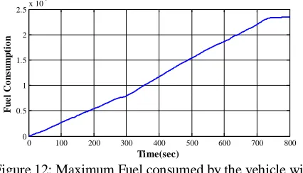
The maximum amount of hydrogen consumed by the proposed vehicle with the use of M-HWY drive cycle pattern is 2.4 grams and the fuel consumption graph is shown in Fig. 12.
0 100 200 300 400 500 600 700 800
0 0.5 1 1.5 2 2.5x 10
-3
Time(sec)
F
ue
l C
o
ns
um
pt
io
n
Figure 12: Maximum Fuel consumed by the vehicle with the M-HWY Drive Cycle Pattern
The maximum distance covered by the vehicle at the end of the M-HWY drive cycle pattern is 4600m and it is shown in Fig. 13.
0 100 200 300 400 500 600 700 800
0 1000 2000 3000 4000 5000
Time(sec)
D
is
p
la
cem
en
t(
m
)
Figure 13: Maximum Distance Coverage by the vehicle with the M-HWY Drive Cycle Pattern
M-FTP DRIVING CYCLE
The FTP (Federal Test Procedure) heavy-duty transient cycle is used for regulatory emission testing of heavy-duty on-road engines in the United States. The FTP transient test is based on the
0 200 400 600 800 1000 1200 1400 1600 1800
0 10 20 30 40 50 60
Time(sec)
Spe
e
d(
km
/hr
)
chassis dynamometer driving cycle. The cycle includes “motoring” segments and, therefore, requires a DC or AC electric dynamometer capable of both absorbing and supplying power. The transient test was developed to take into account a variety of heavy-duty truck and bus driving patterns in American cities, including traffic in and around the cities on roads and expressways. The variation of normalized speed and torque with time is shown in Fig. 14.
Figure 14
:
M-FTP Driving Cycle PatternThe comparison between the required vehicle power and the power delivered from the energy source (fuel cell) with the M-FTP drive cycle pattern is shown in Fig. 15.
0 200 400 600 800 1000 1200 1400 1600 1800
-2000 -1000 0 1000 2000 3000 4000
Time(sec)
P
o
w
e
r
(w
a
tts
)
Power Required Power Delivered
Figure 15 Power Flow within the vehicle for M-FTP Driving Cycle Pattern
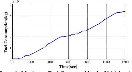
The maximum amount of fuel consumed by the vehicle at the end of the M-FTP drive cycle pattern is 9*10-3
0 200 400 600 800 1000 1200 1400 1600 1800
0 0.002 0.004 0.006 0.008 0.01
Time(sec)
F
ue
l C
o
ns
um
pt
io
n(
kg
)
kg and it is represented in Fig. 16.
Figure 16: Fuel Consumption by the vehicle with the M-FTP Driving Cycle Pattern
The maximum distance covered by the vehicle at the end of the M-FTP drive cycle pattern is 11000m and it is shown in Fig. 17
.
0 200 400 600 800 1000 1200 1400 1600 1800
0 2000 4000 6000 8000 10000 12000
Time(sec)
D
is
p
la
c
em
en
t(
m
)
Figure 17: Maximum Distance coverage with the M-FTP Driving Cycle Pattern
161
Copyright © 2011-15. Vandana Publications. All Rights Reserved.
V.
CONCLUSION
The complexity involved in developing the conventional mathematical modeling of fuel cell is defeated with the advent of an artificial intelligent technique. The standalone fuel cell powered electric vehicle model developed in this paper includes the modeling of fuel cell, unidirectional converter modeling and vehicle dynamics modeling. From the simulation results, it is clear that the proposed electric vehicle model provides the exact prediction performance in terms of power flow, maximum distance coverage and maximum amount of fuel consumed by the proposed vehicle. The proposed method when implemented provides complete solution for global warming and rise in emissions. But some of the practical issues included with the standalone fuel cell operated electric vehicle such as cold start problems, amount of fuel consumption and loss of regenerative power etc., are not discussed in this paper. Also, the proposed electric vehicle model is used only for low power applications and hence the future studies will be focused on developing fuel cell based hybrid electric vehicle models that include batteries or ultra-capacitors as a backup source for providing high power.
REFERENCES
[1] M. Karthik and S. Vijayachitra, “An integrated exploration of thermal and water management dynamics on the performance of a stand-alone 5-kW Ballard fuel cell system for its scale-up design,” Proceedings of the Institution of Mechanical Engineers, Part A: Journal of Power and Energy, vol. 228, pp. 836-852, 2014.
[2] Sudaryono, Soebagio and Mochamad Ashari, “Neural Network Model of Polymer Electrolyte Membrane Fuel Cell for Electrical Vehicle”, Journal of Theoretical and Applied Information Technology, vol. 49, pp. 32-37, 2013. [3] Pooja Sharma and Amita Mahor, “A New PWM Based Soft Switching for DC/DC Converter,” VRSD International Journal for Electrical, Electronics and Communication Engineering, vol. 2, no. 3, 2012.
[4] K. Mammar and A. Chaker, “Neural Network-Based Modeling of PEM fuel cell and Controller Synthesis of a stand - alone system for residential application,” International Journal of Computer Science Issues (IJCSI), vol. 9, pp. 244-253, 2012.
[5] Martin T. Hagan and Mohammad B. Menhaj, “Training Feed forward Networks with the Marquardt Algorithm,” IEEE Trans. Power Neural Network, vol.16, pp.78-84, Jan.2008.
[6]BP Statistical Review of World Energy, June 2007, www.bp.com/statisticalreview.
[7] Bruce Lin, “Conceptual design and modeling of a fuel cell scooter for urban Asia,” Elsevier Journal of Power Sources, vol. 86, pp. 202–213, 2000.