www.nonlin-processes-geophys.net/22/601/2015/ doi:10.5194/npg-22-601-2015
© Author(s) 2015. CC Attribution 3.0 License.
A framework for variational data assimilation
with superparameterization
I. Grooms1,2and Y. Lee1
1Center for Atmosphere Ocean Science, Courant Institute of Mathematical Sciences, New York University, New York, USA 2Department of Applied Mathematics, University of Colorado, Boulder, Colorado, USA
Correspondence to: I. Grooms ([email protected])
Received: 9 March 2015 – Published in Nonlin. Processes Geophys. Discuss.: 20 March 2015 Revised: 25 August 2015 – Accepted: 28 September 2015 – Published: 9 October 2015
Abstract. Superparameterization (SP) is a multiscale com-putational approach wherein a large scale atmosphere or ocean model is coupled to an array of simulations of small scale dynamics on periodic domains embedded into the com-putational grid of the large scale model. SP has been success-fully developed in global atmosphere and climate models, and is a promising approach for new applications, but there is currently no practical data assimilation framework that can be used with these models. The authors develop a 3D-Var variational data assimilation framework for use with SP; the relatively low cost and simplicity of 3D-Var in comparison with ensemble approaches makes it a natural fit for relatively expensive multiscale SP models. To demonstrate the assim-ilation framework in a simple model, the authors develop a new system of ordinary differential equations similar to the two-scale Lorenz-’96 model. The system has one set of vari-ables denoted{Yi}, with large and small scale parts, and the SP approximation to the system is straightforward. With the new assimilation framework the SP model approximates the large scale dynamics of the true system accurately.
1 Introduction
Superparameterization (SP) is a multiscale computational method for parameterizing small scale effects in large scale atmosphere and ocean models. It was originally developed and has been particularly effective as a cloud parameteriza-tion in atmosphere models (Grabowski and Smolarkiewicz, 1999; Randall et al., 2003), and has been implemented in global atmosphere and climate models (Khairoutdinov and Randall, 2001; Tao et al., 2009; Randall et al., 2013). SP
cou-ples a large scale, low resolution model to an array of local small scale, high resolution simulations embedded within the computational grid of the large scale model. The computa-tional cost is kept down through a variety of methods, most prominently by reducing the dimensionality of the small scale simulations, e.g., using one vertical and one horizontal coordinate in the aforementioned atmospheric applications. Although atmosphere and climate models with SP are partic-ularly successful at producing a realistic Madden-Julian os-cillation and diurnal cycle of convection over land (Khairout-dinov et al., 2005), there are as yet no data assimilation sys-tems designed for use with these models. Instead, the large scale variables are initialized from state estimates generated with non-SP models and the small scale variables are initial-ized with small-amplitude noise (Khairoutdinov et al., 2005). Once the SP model has been initialized, there is no practical framework for combining observational data with the multi-scale model forecast to produce a new initial condition.
these models with the framework of GLM14 in the near fu-ture. Here we develop a 3D-Var variational data assimilation framework for SP that builds on and modifies the framework of GLM14.
Observations of physical variables have large scale and small scale parts, the former of which is equated with the large scale model variables, and the latter with the variables of the small scale embedded simulations. A key feature of SP is that the small scale simulations are periodic, so a location on the small scale computational grid does not correspond precisely to any location in the real physical domain; as a result, the small scale simulations provide only statistical in-formation about the small scales, and this inin-formation can be used as a prior in the data assimilation context. In GLM14 an ensemble of SP simulations provides prior information on the large scale variables, but in the present approach the prior information on the large scales comes from a single SP simulation and a time-independent “background” covari-ance matrix for the large scale variables. When the observa-tion operator is linear the analysis estimates of the large and small scale variables can be computed independently of each other, and the small scale covariance information effectively provides a time- and state-dependent estimate of represen-tation error. When the observation operator is nonlinear the large and small scale analysis must be computed simultane-ously by minimizing an objective function. Although anal-ysis estimates of the small scale variables can be computed with linear observations, and must be computed with nonlin-ear observations, our framework does not at this time use the small scale analysis estimate to update any of the small scale SP variables because the latter cannot be unambiguously as-sociated with any real physical location. A key update of the GLM14 framework is that we here compute a small scale analysis estimate at locations where observations are avail-able, rather than at every coarse grid point. This can result in significant computational savings in the case of a nonlinear observation operator. We also update the GLM14 framework to better handle observations at locations off the coarse grid. The complex superparameterized atmosphere and climate models mentioned above are not particularly convenient for the development of a new data assimilation framework, and existing toy models of SP are of limited utility for this pur-pose. In Sect. 2 we develop a new system of ordinary dif-ferential equations based on the two-scale Lorenz-’96 (L96) model (Lorenz, 1996, 2006), and an SP approximation to that system. This new model serves as a test bed in which to demonstrate our new SP 3D-Var framework. The 3D-Var framework with SP is presented in Sect. 3, and assimilation experiments using the new framework and the new system are described in Sect. 4, followed by conclusions.
2 A multiscale Lorenz-’96 model with superparameterization
In this section we develop a new simple model for SP in which to demonstrate our data assimilation framework. Ma-jda and Grote (2009) developed an idealized model of SP, but the system suffers from one major drawback: it does not consist of an SP approximation to an idealized system, but rather consists only of an idealized SP model. Harlim and Majda (2013) used the model of Majda and Grote (2009) to develop a data assimilation strategy for SP, but with the as-sumption that direct observations of the large scale variables were available, rather than having both large and small scale contributions to the observations. Lee and Majda (2015) have recently investigated a range of multiscale assimilation meth-ods in a highly condensed model where the “large scale” con-sists of a single scalar with no spatial extent.
Wilks (2012) developed an SP approximation for the two-scale Lorenz-’96 system, which has the following form (Lorenz, 1996, 2006):
˙
Xk= −Xk−1(Xk−2−Xk+1)−Xk− hc
b J
X
j=1
Yj,k+F (1)
˙ Yj,k=c
−bYj+1,k Yj+2,k−Yj−1,k−Yj,k+ h bXk
. (2) The Xk variables have periodicity Xk=Xk+K, and the Yj,k variables have periodicity Yj+J,k=Yj,k+1 and Yj,k+K=Yj,k, where j=1, . . . ,J andk=1, . . . ,K. The combined index j+J (k−1) is naturally associated with spatial location along a latitude circle, and the local aver-ageJ−1
J
P
j=1
serves to separate large and small spatial scales. This system is primarily useful as a two-timescale model, since for large c the Yj,k variables are faster than the Xk variables. Wilks’s SP approximation to this system reflects this fact by treating theYj,kvariables as purely small-scale; also, in his SP approximation the periodicity of theYj,k vari-ables is replaced by definingY0,k=YJ+1,k=YJ+2,k, which
are set to a constant value. Considering that the multiscale nature of SP is primarily based on spatial scale separation rather than timescale separation, a more natural SP approx-imation to the two-scale Lorenz-’96 system might make the Yj,k variables locally periodic:Yj+J,k=Yj,k. Nevertheless, there would still be two sets of large scale variables (Xk, and thej-average ofYj,k) but only one set of small scale vari-ables (Yj,k minus itsj average). Rather than bend the two-timescale Lorenz-’96 model to our two-space-scale purpose, we develop a new two-space-scale version of the Lorenz-’96 model that is more naturally suited to an SP approximation.
The new model is defined by the following equation:
˙
indexi, which is periodicYi+J K=Yi, is analogous to spatial location on a latitude circle, similar to the original L96 model (Lorenz, 1996, 2006). The nonlinear functions NY andNX are defined as
{NY(Y)}i = −Yi+1(Yi+2−Yi−1) , (4) {NX(X)}k= −Xk−1(Xk−2−Xk+1) , (5)
where Eqs. (4) and (5) are evaluated assuming periodic-ity for the vectors X= {Xk}Kk=1 and Y: Xk+K=Xk and Yi+J K=Yi. The matrix T extracts the large scale part ofY; we choose to let T be defined as the projection onto the first K discrete Fourier modes, followed by evaluation on an eq-uispaced grid ofKpoints. The large scale dynamics are ob-tained by applying T to Eq. (3) from the left:
˙
X=hTNY(Y)+NX(X)−X+F1K, (6) where we define the large scale component X=TY, and use thatJT TT is the identity matrix and that T 1J K=1K (these are true for our choice of a Fourier projection, but other choices of T are possible). Note that when h=0 the dynamics are those of the single-scale Lorenz-’96 model with K modes, and when h6=0 the nonlinearity NY(Y) couples large and small scales. Energy conservation for the nonlinear terms in Eq. (3) is obtained by noting that Eq. (4) implies YTNY(Y)=0, and that Eq. (5) implies YTTTNX(TY)=XTNX(X)=0. The matrix JTT inter-polates fromRKtoRJ K, and it is convenient to define
nota-tion for the small scale part ofY: y= {yi}J Ki=1=Y−JT
TTY. (7)
The superparameterization approximation is governed by
˙
Yj,k= −hYj+1,k Yj+2,k−Yj−1,k
−Xk−1(Xk−2−Xk+1)−Yj,k+F, (8)
where Xk=J−1 J
P
j=1
Yj,k, and there is local as well as global periodicity:Yj+J,k=Yj,kandXk+K=Xk. The large scale dynamics in the SP approximation are obtained byj -averaging Eq. (8), which gives
˙ Xk= −
h J
J
X
j=1
Yj+1,k Yj+2,k−Yj−1,k
−Xk−1(Xk−2−Xk+1)−Xk+F. (9) Whenh=0 the large scale dynamics of the SP approxima-tion and the true system are equivalent. As in more complex SP applications, the small scale variables (here Yj,k−Xk) are locally periodic, and are coupled to the large scale using a local average over a periodic domain in a manner analogous to the coupling in more complex SP models (e.g., Grabowski, 2004). The Xk variables in the SP model attempt to accu-rately model the dynamics of Xin the true system, but the
small scale variables of the SP approximation are only statis-tically related to the small scale variables of the true system; i.e., one does not expect an SP variableYj,k to be a direct approximation of any of the true system variablesYi.
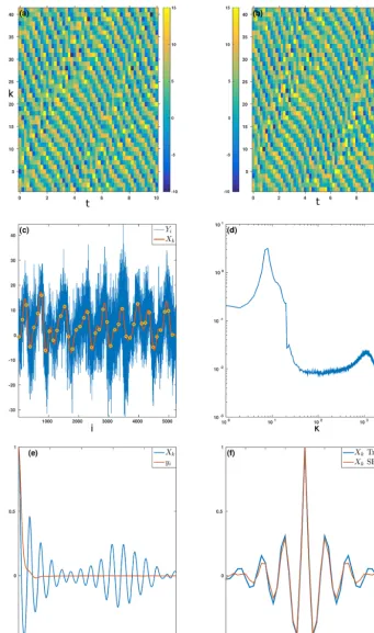
The purpose of this research is not to study the SP ap-proximation in this system, but rather to use the system as a test bed for our data assimilation framework. We therefore choose to focus on parameter regimes where the SP approxi-mation is reasonably accurate, settingJ=128 so that there is a good scale separation (the SP approximation should break down for smallJ). The number of large scale modes is set to K=41; we choose 41 rather than the usual 40 so that the dis-crete Fourier modes associated with the large scale variables are 0,±1, . . . ,±20, and the twentieth mode is not split be-tween large and small scales. It remains to chooseFandh. In general, for fixed nonzerohthe small scale variables become more chaotic and larger amplitude asF increases, and simi-larly for fixedF ashincreases. As the small scales become more chaotic and larger amplitude, the large scale variables become less chaotic. This behavior is perhaps counterintu-itive, but similar behavior has been observed in the two-scale Lorenz-’96 system by Abramov (2012). Balancing the desire for complex large scale dynamics and turbulent small scale dynamics, we choose to focus on two parameter regimes:
I. F=30,h=0.4; II. F=21,h=0.35.
Some characteristics of the dynamics in regimes I and II are presented in Figs. 1 and 2, respectively. In regime I the large scale dynamics consist of a train of eight propagating and nonlinearly interacting “waves”, as seen in the time se-ries of theXvariables in Fig. 1a. The large scale dynamics of the SP approximation are qualitatively similar, as shown in Fig. 1b. The time-lagged autocorrelation function of the Xk variables (averaged overk) is shown in Fig. 1e, and dis-plays an oscillatory structure associated with the wave train. The initial decay of the time-lagged autocorrelation is ap-proximated by an exponential of the form exp{−(λ+iω)t}
Fourier modes (κ≤20) and the small scale modes, showing that the large scale energy is concentrated near wave numbers κ=7 and 8, while the small scale energy is more broadly distributed among Fourier modes. The broad distribution of small scale energy among Fourier modes is indicative of the strongly chaotic small scale dynamics, as is the rapid tem-poral decorrelation of the small scale variablesyi shown in Fig. 1e. The decorrelation time of the small scale variables yi is estimated as 0.2 using the integral of the time-lagged autocorrelation function.
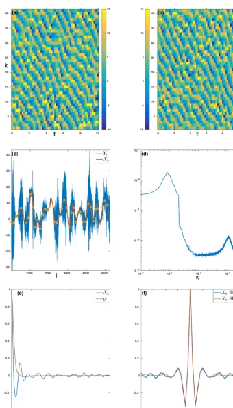
In regime II the large scale dynamics are more chaotic, though wave trains are still evident in the time series of X in Fig. 2a. The large scale dynamics of the SP approxima-tion are again qualitatively similar, as shown in Fig. 2b. The time-lagged autocorrelation function of the Xk variables in Fig. 2e decays much more rapidly than in regime I. The ini-tial decay of the time-lagged autocorrelation is approximated by an exponential of the form exp{−(λ+iω)t}with decor-relation timeλ−1=0.38 and oscillation period 2π/ω=0.95, and there is no resurgence of correlations at long lag times. The decreased regularity of the wave train is reflected in the space-lagged autocorrelation function for the Xk variables shown in Fig. 2f, which is again well approximated by the SP dynamics. The snapshot of the Yi variables in Fig. 2c shows a diminished level of small scale variability overall, with some regions having almost no small scale activity and others having strong small scale variability. The energy spec-trum in Fig. 2d shows that the energy is more broadly dis-tributed among large scale Fourier modes, though there is still a peak at wave numberκ=8. The broad distribution of small scale energy among Fourier modes is again indicative of the strongly chaotic small scale dynamics, as is the rapid temporal decorrelation of the small scale variablesyi shown in Fig. 2e. The decorrelation time of the small scale variables yi is estimated as 0.23 using the integral of the time-lagged autocorrelation function.
TheYi variables have a uniform time mean of 3.8 and 3.6 in regimes I and II, respectively, which is accurately repro-duced by the SP approximation. TheXkvariables have vari-ance 31 and 32 in regimes I and II, respectively, and their SP counterparts have slightly higher variances of 33 and 34. The small scale variablesyihave climatological variance of 70 in regime I and 29 in regime II, though Figs. 1c and 2c show that this variability is unevenly distributed over the physical domain at any given instant.
3 Variational data assimilation with superparameterization
The primary difficulty in developing a data assimilation framework for an SP model is that observations of the true system include contributions from large and small scales, and it is necessary to relate the observations to the large and small scale variables of the SP model. GLM14 provided a
frame-work for relating observations to SP model variables, and we improve on this framework below.
Let the large scale variables of the SP simulation be de-notedu(the overbar does not denote a statistical mean), and let the small scale variables be denotedeu. In the context of the new Lorenz-’96 model,u=Xandeu= {Yj,k−Xk}j,k. In most SP applications there is a set of small scale variables at every point of the large scale computational grid. The small scale variables exist on local periodic domains so that the small scale variables at each coarse grid point are discon-nected from those at surrounding coarse grid points, and the small scale variables have zero average across the periodic directions. Each location in the small scale periodic domains does not correspond to a different location in the real phys-ical domain. Instead, all points in a given periodic domain are best thought of as existing at one physical location: the associated coarse grid point.
In GLM14, observations are related to the SP model vari-ables using the following observation model
v=H(L(u+u0))+ε, (10)
whereH is the observation operator andεis a vector of zero-mean normal random variables associated with observation error. The vectoru0has the same size asu, and models the small scale contribution to physical variables at the coarse grid points; i.e.,u=u+u0is the vector of real physical vari-ables at the coarse model grid points. The physical varivari-ables uare interpolated to the location of the observations by L. The vectoru0is not the same as the small scale SP variables
eu. Instead, the mean and covariance ofu
0are computed from the statistics of the small scale SP variableseu. Although the true small scale variablesu0 can in principle have nonzero statistical mean, the small scale SP variableseualways have zero mean because their average over the local periodic do-mains is always zero by definition. For example, in the con-text of the new Lorenz-’96 model the GLM14 version of the vectoru0 has lengthK, has zero mean, and has a diagonal covariance with entries
Varu0k= 1 J−1
J
X
j=1
Yj,k−Xk
2
. (11)
be smoothly interpolated from the coarse grid points, where small scale SP statistics are available, to the locations of the observations.
Let P denote the number of different physical locations where observations are available (for simplicity of exposi-tion, we assume that there is only one observation per lo-cation, i.e.,v∈RP). The updated observation model for the pth location is
vp=Hp
Lp(u)+u0p
+εp, (12)
where Lpinterpolates the large scale model variablesuto the observation location andεpis a zero-mean Gaussian random variable. There is thus one vectoru0pof small scale variables per observation location. The updated observation model for allP observations can be written in vector form as
v=H(L(u)+u0)+ε, (13)
whereu0is no longer defined as in GLM14, but according to the discussion above.
The covariance of the small scale variables P0 is com-puted from the small scale variables of the SP model, and thus changes from one assimilation cycle to the next. Specif-ically, it is first assumed that the small scale variables at dif-ferent observation locations are uncorrelated from each other so that one needs only compute the covariance matrices P0pof theu0pvariables. This assumption is reasonable as long as the observations are taken at locations reasonably well separated compared to the correlation length of the small scale vari-ables. (The framework could be updated for situations where the observations are closer than this, e.g., by using spatial correlation information for the small scale variables com-puted from the SP simulation, but this is beyond the scope of the present investigation.) To compute P0p we begin by computing auxiliary small scale sample covariance matrices
e
Pk using the small scale SP variableseuat each coarse grid
point. Let{ euk,j}
J
j=1be the small scale SP variables located
in a periodic domain at thekth coarse grid point, where there areJgrid points in the periodic embedded domain. Then, re-calling that their average overJ is zero, the auxiliary small scale sample covariance matrix is
e
Pk= 1 J−1
J
X
j=1 euj,keu
T
j,k, (14)
where the superscriptT denotes a vector transpose. It is typ-ically the case that J is large enough thatePk is full rank, and we do not consider exceptions here. In the context of the new Lorenz-’96 model the auxiliary small scale sample covariances are given by Eq. (11). Finally, the small scale covariance matrices at the observation locations P0p are ob-tained by interpolating the elements of the matricesePk from the coarse grid to the locations of the observations, which assumes that the small scale statistics vary smoothly on the
large scale. The interpolation method used to interpolate the small scale covariance matrices need not be the same as L, and should have positive coefficients in order to ensure that the small scale covariance matrices remain positive definite. (It may not be necessary to compute sample covariance ma-tricesePkat every coarse grid point; one only needs to com-pute them at points needed in the interpolation.) For compar-ison, in GLM14 the covariance of the small scale variables P0 is the same size as the large scale background covariance B, and consists of the auxiliary small scale sample covariance matricesePk arranged in block-diagonal form. When obser-vations are taken at every coarse grid location the GLM14 formulation is equivalent to the new one.
To complete the specification of the 3D-Var framework we specify a prior joint distribution foruandu0with mean
E[u] =µ, E[u0] =0 (15)
and covariance
B 0
0 P0
. (16)
As typical in a 3D-Var setting, the background covariance matrix B for the large scale variables is independent of time, and the prior mean for the large scales is given by a single forecast of the large scale part of the SP model. The small scale variableu0is assumed to be uncorrelated with the large scale variable. In practice, the large and small scale variables are certainly not independent, but as shown in GLM14 the assumption that they are uncorrelated is reasonable within the context of an SP model where the small scale variables have zero mean. To wit, the joint probability distribution of large and small scale variables can be factored into the large scale marginal and the small scale conditional distributions p(u,u0)=pM(u) pC(u0|u). The cross-covariance between large and small scale variables is
Z Z
(u−µ)u0TpM(u)pC(u0|u)dudu0
= Z
(u−µ)pM(u)
Z
u0TpC(u0|u)du0
du=0, (17) where the term in square brackets is zero because the small scale variables are assumed to have zero mean regardless of the state of the large scale variables.
Having thus specified the observation model and prior mean and covariance, the 3D-Var analysis estimate of the system state minimizes the following objective function (Ta-lagrand, 2010):
ϒ (u,u0)=(u−µ)TB−1(u−µ)+u0TP0−1u0
When the observation operator is linear,H=H, the anal-ysis can be computed from the Kalman filter formulas (Tala-grand, 2010), which in this case gives
ua=µ+K(v−HLµ), (19)
K=B(HL)THLB(HL)T+HP0HT +R −1
, (20)
u0a=K0(v−HLµ), (21)
K0=P0HTHLB(HL)T +HP0HT +R −1
, (22)
where the superscript “a” denotes the analysis estimate. A key feature of these formulas is that the large scale and small scale estimates can be computed independently. In particular, the large scale estimate can also be computed as the mini-mizer of the following objective function:
ϒ (u)=(u−µ)TB−1(u−µ)
+(v−HLu)THP0HT +R −1
(v−HLu). (23) In cases where the small scale estimate is not used and the ob-servation operator is linear, the small scale estimate does not need to be computed. It can be seen from Eqs. (20) and (23) that the observed small scale covariance matrix H P0HT acts as a time-varying estimate of the representation error since it inflates the measurement error covariance R.
In GLM14 the small scale covariance matrix P0is defined differently (as described above) and the small scale vectoru0 is the same size as the large scale vectoru. In the GLM14 formulation the final term in the objective function Eq. (18) is replaced by
(v−H(L(u+u0)))TR−1(v−H(L(u+u0))). (24) For linear observations the GLM14 versions of the Kalman filter formulas are
ua=µ+K(v−HLµ) (25)
K=B(HL)THL(B+P0)(HL)T +R −1
(26)
u0a=K0(v−HLµ) (27)
K0=P0(HL)T
HL(B+P0)(HL)T +R −1
. (28)
In the new approach there is one set of small scale variables for each location where observations are available, whereas in GLM14 there are small scale variables at each coarse grid point. In global atmosphere and climate models there are typically fewer observations than coarse grid points; when the observation operator is nonlinear the new formulation is more efficient because the objective function has fewer de-grees of freedom. Another key difference is in the assump-tions that go into the specification of the small scale back-ground covariance: in GLM14 the small scale variables are tacitly assumed to vary smoothly over the physical domain,
since they are smoothly interpolated between coarse grid points, whereas in the present approach only the small scale covariance is assumed to vary smoothly over the domain.
4 Assimilation experiments
In this section we describe data assimilation experiments in both regimes of the test model using the 3D-Var framework from Sect. 3.
Observations are taken at P=MK equispaced points with M=1, 2, and 4; specifically, observations are taken at ip=1+pJ /M for p=1, . . . , P. Observations are either linear, with vp=Yip+εp, or nonlinear, with vp=(Yip+30)2/50+εp. In both cases the observation er-rorsεp are iid Gaussians with zero mean and variance 0.1. Observations are assimilated every1ttime units. In regime I we test 1t=0.2 and 0.6; for comparison the decorrela-tion times of the small scale and large scale variables in this regime are 0.2 and 0.84. In regime II we test1t=0.2 and 0.4, which are close to the decorrelation times of the small scale and large scale variables, respectively.
Specification of the background covariance matrix is a cru-cial aspect of any 3D-Var assimilation system. We consider the simplest possible estimate B=σ2IK where IK is the K×K identity matrix andσ2is a tunable parameter. Assimi-lation experiments are run over a range ofσ2and the optimal value is chosen based on rms (root mean square) errors; the results are very weakly sensitive toσ2as long as it is within a factor of 2 of the diagnosed forecast error variance. Since our observing system includes at least one observation for every Xkvariable, it is less important to build a background covari-ance matrix with correlations between theXkvariables.
A single assimilation experiment consists of 1000 cycles, where the SP variables for the first forecast are initialized directly from the true model variables. Although the assim-ilation system provides estimates of the small scale part of the true system at the location of the observations, this infor-mation is far from sufficient to provide an estimate of the full stateY of the true system. We view the 3D-Var assimilation as primarily aimed at estimating the large scale model vari-ablesXk, and error statistics are tracked only for the large scale variables. We track two performance metrics for the large scale variables, the time averaged rms error
rms error= |X−XSP|2 (29)
and the time averaged pattern correlation
Pattern correlation= X
TXSP
|X|2|XSP|2 (30)
both for the forecast and for the analysis.
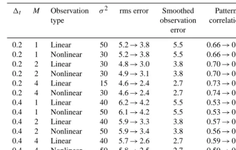
Table 1. Results of the assimilation experiments for regime I. There areP=MKequispaced observations, assimilated at time intervals of1t, andσ2is the amplitude of the background covariance matrix. For comparison, the climatological rms error and pattern correlation are 5.6 and 0.57.
1t M Observation σ2 rms error Smoothed Pattern
type observation correlation
error
0.2 1 Linear 15 4.9→4.3 8.2 0.73→0.79
0.2 1 Nonlinear 20 4.7→4.1 8.1 0.74→0.80
0.2 2 Linear 10 4.1→3.4 5.7 0.81→0.87
0.2 2 Nonlinear 20 4.2→3.4 5.7 0.80→0.87
0.2 4 Linear 10 3.4→2.6 4.1 0.87→0.92
0.2 4 Nonlinear 15 3.8→2.8 4.0 0.83→0.91
0.6 1 Linear 35 6.1→5.1 8.2 0.60→0.72
0.6 1 Nonlinear 40 5.6→4.8 8.2 0.63→0.74
0.6 2 Linear 30 5.5→4.2 5.7 0.66→0.82
0.6 2 Nonlinear 30 5.2→4.0 5.7 0.68→0.82
0.6 4 Linear 25 5.0→3.3 4.1 0.72→0.89
0.6 4 Nonlinear 30 4.8→3.2 4.0 0.73→0.89
the uniform climatological mean value ofXkas a prediction: Xk=3.8 in regime I andXk=3.6 in regime II. The clima-tological rms error is simply the square root of the climato-logical variance: 5.6 in regime I and 5.7 in regime II. The climatological pattern correlation is the time averaged pat-tern correlation between Xk and its uniform climatological mean value: the climatological pattern correlation is 0.57 in regime I and 0.53 in regime II. If the forecast has a larger rms error or smaller pattern correlation than the climatologi-cal values, then the forecast is of very limited utility.
As a point of comparison for the performance of the analysis estimate in the assimilation experiments we take a “smoothed observation” estimate that is obtained by pro-jecting the observations onto the largest K Fourier modes. For example, whenM=1 there areKobservations and the “smoothed observation” estimate of theXk variables is sim-ply Xk≈vp for the linear case and Xk≈p50vp−30 for the nonlinear case. The rms errors in the smoothed obser-vation estimate are tracked over the course of each assimi-lation experiment, rather than computing climatological val-ues. The 3D-Var should at a minimum perform better than the smoothed observations. The results for both regimes are pre-sented in Tables 1 and 2 in the format Forecast→Analysis. In all cases the errors decrease asMincreases, and the analysis significantly improves over the forecast.
We also compare to the performance of an ensemble adjustment Kalman filter using the true system dynamics. These experiments and their results are described in Section “Comparison to EAKF”.
The large scale dynamics are more predictable in regime I than in regime II, but the small scale variance is larger as well, making it harder to obtain an accurate estimate of the large scales. With a short observation time1t=0.2, the fore-cast and analysis for linear and nonlinear observations both have rms errors smaller than both the climatological error
Table 2. Results of the assimilation experiments for regime II. There areP=MKequispaced observations, assimilated at time in-tervals of1t, andσ2is the amplitude of the background covariance matrix. For comparison, the climatological rms error and pattern correlation are 5.7 and 0.53.
1t M Observation σ2 rms error Smoothed Pattern
type observation correlation
error
0.2 1 Linear 50 5.2→3.8 5.5 0.66→0.83
0.2 1 Nonlinear 30 5.2→3.8 5.5 0.66→0.83
0.2 2 Linear 30 4.8→3.0 3.8 0.70→0.89
0.2 2 Nonlinear 30 4.9→3.1 3.8 0.70→0.89
0.2 4 Linear 15 4.6→2.4 2.7 0.73→0.93
0.2 4 Nonlinear 30 4.6→2.4 2.7 0.74→0.94
0.4 1 Linear 40 6.2→4.2 5.5 0.53→0.79
0.4 1 Nonlinear 50 6.1→4.2 5.5 0.53→0.80
0.4 2 Linear 40 5.9→3.3 3.8 0.57→0.87
0.4 2 Nonlinear 50 5.9→3.4 3.8 0.56→0.87
0.4 4 Linear 40 5.7→2.6 2.7 0.59→0.92
0.4 4 Nonlinear 50 5.8→2.5 2.7 0.59→0.93
of 5.6 and the error in the smoothed observation estimate. The nonlinear observations generate slightly more accurate results than the linear observations whenM=1, and the lin-ear observations generate slightly more accurate results for M=4, but overall the results are similar. With a longer ob-servation time1t=0.6 the results are, naturally, less accu-rate. In every case the analysis is more accurate than both the climatological error and the smoothed observations, but the forecasts are more accurate than the climatological mean only withM=4. WithM=1 and 2, the rms forecast errors are worse than the climatological error, but the forecast pat-tern correlations are still a bit better than the climatological pattern correlation. As with the shorter observation time, the results are more accurate with the nonlinear observations.
In regime II the results with the linear and nonlinear obser-vations are very similar in all cases. With a short observation time1t=0.2, the forecast is always more accurate than the climatological mean, and the analysis is always more accu-rate than the smoothed observations. With a longer observa-tion time1t=0.4 the forecasts are no more accurate than climatology, but the analysis is still more accurate than the smoothed observations, though atM=4 the analysis is only slightly more accurate.
Comparison to EAKF
and Cohn, 1999), and optimal results were obtained with 5 % inflation and a localization radius of four grid points.
In regime I the rms forecast errors of the Xk variables were 5.1, decreasing to 4.6 after the analysis; the rms forecast pattern correlation was 0.61, improving to 0.69 after the anal-ysis. In regime II the rms forecast errors of theXkvariables were 5.9, decreasing to 5.6 after the analysis; the rms fore-cast pattern correlation was 0.53, and remained essentially unchanged at 0.52 after the analysis.
In both regimes the EAKF estimates the large scale part of the solution very poorly, much worse than the SP 3D-Var. This poor performance is presumably associated with the fact that the EAKF is attempting to estimate the full system state Y, whereas the SP 3D-Var is only estimating the large scale part. From the point of view of the EAKF the observations are very sparse, since there is only one observation for every 32 variables, whereas from the point of view of the SP 3D-Var there are four observations for every large scaleXk vari-able. The significant improvement in both cost and accuracy of using the SP 3D-Var instead of a perfect-model ensemble Kalman filter underscores the utility of the present approach, though it bears noting that one should be very hesitant to ex-trapolate results such as these to the far more complex setting of SP atmosphere models. Furthermore, whether or not SP 3D-Var will be more accurate than a state of the art ensemble Kalman filter in an atmospheric model context is somewhat beside the point since the goal here is to provide a practical framework for data assimilation with SP models where no such framework currently exists.
5 Conclusions
Superparameterization (SP) is a multiscale computational approach that has been successfully applied to modeling at-mospheric dynamics, and that shows promise for more gen-eral applications (Tao et al., 2009; Randall et al., 2013; Ma-jda and Grooms, 2014). Grooms et al. (2014) have devel-oped an ensemble Kalman filter framework for use with SP. However, the standard approach to SP in global atmosphere and climate models, where small scale nonlinear dynamics are simulated on an array of periodic domains embedded in the computational grid of a large scale model, is too com-putationally demanding for use in an ensemble framework. As a result, there is at present no practical framework for data assimilation with SP models. We here develop a 3D-Var variational data assimilation framework for SP that builds on and modifies the framework of GLM14. The main up-date to the GLM14 framework, in addition to using a vari-ational as opposed to ensemble Kalman filter setting, is that small scale estimates are computed at locations where ob-servations are taken, rather than at every point of the large scale model’s computational grid. The computational costs of the new framework are such that it could be used with
computationally demanding global atmosphere and climate SP models.
The data assimilation framework is demonstrated in a new system of ordinary differential equations based on the two-scale Lorenz-’96 model (Lorenz, 1996, 2006). Unlike the two-scale Lorenz-’96 model the new model has only one set of variables,Yi, and these variables have large and small scale parts. An SP approximation to the new system is devel-oped, which is perhaps the simplest idealized model of SP. The new data assimilation framework is tested in two regimes of the new model, with both linear and nonlinear observation operators. In regime I the large scale dynamics consist of a weakly chaotic wave train, with relatively strong small scale variability superposed. In regime II the large scale dynam-ics are more strongly chaotic, and there is less small scale variability. In both regimes the data assimilation performs as expected (and better than an ensemble Kalman filter using 100 simulations of the true dynamics), with increased accu-racy as the number of observations increases.
Our work lays a foundation for 3D-Var data assimilation with existing SP models. In order to implement our frame-work with an SP atmosphere or climate model, it would be necessary to specify an appropriate background covariance matrix for the large scale model, but this should be straight-forward given the extensive use of the 3D-Var approach in atmosphere and ocean data assimilation (e.g., Kalnay, 2002; Kleist et al., 2009). In addition, the new framework removes one of the difficulties associated with development of a 3D-Var framework for large scale models: the small scale sim-ulations in the multiscale SP computation provide direct in-formation on the small scale statistics, obviating, or at least simplifying, the need to develop models of representation er-ror.
Author contributions. I. Grooms designed the research, I. Grooms
and Y. Lee carried out the experiments, and I. Grooms prepared the manuscript.
Acknowledgements. The authors acknowledge funding from the
United States Office of Naval Research MURI grant N00014-12-1-0912. The authors thank A. J. Majda for suggesting the addition of a second regime (regime II), and two anonymous reviewers.
Edited by: Z. Toth
Reviewed by: two anonymous referees
References
Abramov, R. V.: Suppression of chaos at slow variables by rapidly mixing fast dynamics through linear energy-preserving coupling, Commun. Math. Sci., 10, 595–624, 2012.
Gaspari, G. and Cohn, S.: Construction of correlation functions in two and three dimensions, Q. J. Roy. Meteorol. Soc., 125, 723– 757, 1999.
Grabowski, W.: An improved framework for superparameterization, J. Atmos. Sci., 61, 1940–1952, 2004.
Grabowski, W. and Smolarkiewicz, P.: CRCP: a Cloud Resolving Convection Parameterization for modeling the tropical convect-ing atmosphere, Physica D, 133, 171–178, 1999.
Grooms, I. and Majda, A. J.: Efficient stochastic superparameteri-zation for geophysical turbulence, P. Natl. Acad. Sci. USA, 110, 4464–4469, doi:10.1073/pnas.1302548110, 2013.
Grooms, I. and Majda, A. J.: Stochastic superparameterization in a one-dimensional model for wave turbulence, Commun. Math. Sci., 12, 509–525, 2014a.
Grooms, I. and Majda, A. J.: Stochastic superparameterization in quasigeostrophic turbulence, J. Comp. Phys., 271, 78–98, 2014b. Grooms, I., Lee, Y., and Majda, A. J.: Ensemble Kalman filters for dynamical systems with unresolved turbulence, J. Comp. Phys., 273, 435–452, doi:10.1016/j.jcp.2014.05.037, 2014.
Grooms, I., Majda, A. J., and Smith, K. S.: Stochastic superparam-eterization in a quasigeostrophic model of the Antarctic Circum-polar Current, Ocean Modell., 85, 1–15, 2015.
Harlim, J. and Majda, A. J.: Test models for filtering with superpa-rameterization, Mult. Model. Simul., 11, 282–308, 2013. Kalnay, E.: Atmospheric modeling, data assimilation, and
pre-dictability, Cambridge University Press, 2002.
Khairoutdinov, M. and Randall, D.: A cloud resolving model as a cloud parameterization in the NCAR Community Climate Sys-tem Model: Preliminary results, Geophys. Res. Lett., 28, 3617– 3620, doi:10.1029/2001GL013552, 2001.
Khairoutdinov, M., Randall, D., and DeMott, C.: Simulations of the atmospheric general circulation using a cloud-resolving model as a superparameterization of physical processes, J. Atmos. Sci., 62, 2136–2154, doi:10.1175/JAS3453.1, 2005.
Kleist, D. T., Parrish, D. F., Derber, J. C., Treadon, R., Wu, W.-S., and Lord, S.: Introduction of the GSI into the NCEP global data assimilation system, Weather Forecast., 24, 1691–1705, 2009.
Lee, Y. and Majda, A. J.: Multiscale methods for data assimilation in turbulent systems, Mult. Model. Simul., 13, 691–173, 2015. Lorenz, E.: Predictability: A problem partly solved, in: Proceedings
of Seminar on Predicability, vol. 1, ECMWF, Reading, UK, 1– 18, 1996.
Lorenz, E.: Predictability: A problem partly solved, in: Predictabil-ity of Weather and Climate, edited by: Palmer, T. and Hagedorn, R., Cambridge University Press, 40–58, 2006.
Majda, A. J. and Grooms, I.: New Perspectives on Superparameter-ization for Geophysical Turbulence, J. Comp. Phys., 271, 60–77, doi:10.1016/j.jcp.2013.09.014, 2014.
Majda, A. J. and Grote, M. J.: Mathematical test models for su-perparameterization in anisotropic turbulence, P. Natl. Acad. Sci. USA, 106, 5470–5474, 2009.
Randall, D., Khairoutdinov, M., Arakawa, A., and Grabowski, W.: Breaking the cloud parameterization deadlock, B. Am. Meteorol. Soc., 84, 1547–1564, 2003.
Randall, D., Branson, M., Wang, M., Ghan, S., Craig, C., Gettel-man, A., and Edwards, J.: A community atmosphere model with superparameterized clouds, EOS, 94, 221–228, 2013.
Talagrand, O.: Variational Assimilation, in: Data Assimilation Mak-ing Sense of Observations, edited by: Lahoz, W., Khattatov, B., and Menard, R., Springer, Berlin, Heidelberg, 41–67, 2010. Tao, W.-K., Anderson, D., Chern, J., Entin, J., Hou, A., Houser, P.,
Kakar, R., Lang, S., Lau, W., Peters-Lidard, C., Li, X., Matsui, T., Rienecker, M., Schoeberl, M. R., Shen, B.-W., Shi, J. J., and Zeng, X.: The Goddard multi-scale modeling system with unified physics, Ann. Geophys., 27, 3055–3064, doi:10.5194/angeo-27-3055-2009, 2009.