Optimal solution error covariance in highly nonlinear problems of variational data assimilation

www.nonlin-processes-geophys.net/19/177/2012/ doi:10.5194/npg-19-177-2012

© Author(s) 2012. CC Attribution 3.0 License.

Nonlinear Processes

in Geophysics

Optimal solution error covariance in highly nonlinear problems of

variational data assimilation

V. Shutyaev1, I. Gejadze2, G. J. M. Copeland2, and F.-X. Le Dimet3

1_{Institute of Numerical Mathematics, Russian Academy of Sciences, 119333 Gubkina 8, Moscow, Russia} 2_{Department of Civil Engineering, University of Strathclyde, 107 Rottenrow, Glasgow, G4 ONG, UK} 3_{MOISE project (CNRS, INRIA, UJF, INPG), LJK, Universit´e de Grenoble, BP 53, 38041 Grenoble, France} Correspondence to: V. Shutyaev (shutyaev@inm.ras.ru)

Received: 6 July 2011 – Revised: 16 February 2012 – Accepted: 20 February 2012 – Published: 16 March 2012

Abstract. The problem of variational data assimilation (DA) for a nonlinear evolution model is formulated as an optimal control problem to find the initial condition, boundary con-ditions and/or model parameters. The input data contain ob-servation and background errors, hence there is an error in the optimal solution. For mildly nonlinear dynamics, the covariance matrix of the optimal solution error can be ap-proximated by the inverse Hessian of the cost function. For problems with strongly nonlinear dynamics, a new statistical method based on the computation of a sample of inverse Hes-sians is suggested. This method relies on the efficient com-putation of the inverse Hessian by means of iterative meth-ods (Lanczos and quasi-Newton BFGS) with precondition-ing. Numerical examples are presented for the model gov-erned by the Burgers equation with a nonlinear viscous term.

1 Introduction

State and/or parameter estimation for dynamical geophysi-cal flow models is an important problem in meteorology and oceanography. Among the few methods feasible for solv-ing these non-stationary large-scale problems, the variational data assimilation (DA) method, called “4D-Var”, is the pre-ferred method implemented at some major operational cen-ters (e.g. Courtier et al., 1994; Fisher et al., 2009). From the mathematical point of view, these problems can be for-mulated as optimal control problems (e.g. Lions, 1986; Le Dimet and Talagrand, 1986) to find unknown control vari-ables in such a way that a cost function related to the obser-vation and a priori data takes its minimum value. A necessary optimality condition leads to the so-called optimality system, which contains all the available information and involves the original and adjoint models. Due to the input errors (back-ground and observation errors), there is an error in the

178 V. Shutyaev et al.: Optimal solution error covariance

the Effective Inverse Hessian (EIH), first introduced by Ge-jadze et al. (2011), to the geophysical research community. The closest concept to this is probably the Expected Fisher Information Matrix used in Bayesian estimation theory.

2 Statement of the problem

Consider the mathematical model of a physical process that is described by the evolution problem

( _∂ϕ

∂t =F (ϕ), t∈(0,T ) ϕ_t=0=u,

(1) whereϕ=ϕ(t )is the unknown function belonging for any t to a Hilbert space X, u∈X, F is a nonlinear opera-tor mapping X into X. Let Y =L2(0,T;X) be a space of abstract functionsϕ(t )with values inX, with the norm kϕk =(

T

R 0

kϕk2

Xdt )1/2. Suppose that for a givenu∈Xthere

exists a unique solutionϕ∈Y to Eq. (1).

Letu¯ be the “exact” initial state and ϕ¯ – the solution to the problem Eq. (1) withu= ¯u, i.e. the “exact” state evolu-tion. We define the input data as follows: the background function ub∈X, ub= ¯u+ξb and the observations y∈Yo, y=Cϕ¯+ξo, whereC:Y →Yo is a linear bounded

oper-ator (observation operoper-ator) and Yo is a Hilbert space

(ob-servation space),ξb∈X,ξo∈Yo. In particular, Yo may be

finite-dimensional (both in space and in time). The random variablesξbandξomay be regarded as the background and the observation error, respectively. Assuming that these er-rors are normally distributed, unbiased and mutually uncorre-lated, we define the covariance operatorsVb· =E[(·,ξb)Xξb] andVo· =E[(·,ξo)Yoξo], where “·” denotes an argument of

the respective operator, andEis the expectation. We suppose thatVbandVoare positive definite, hence invertible.

Let us introduce a cost functionJ (u) J (u)=1

2(V −1

b (u−ub),u−ub)X+

+1 2(V

−1

o (Cϕ−y),Cϕ−y)Yo, (2)

and formulate the following DA problem (optimal control problem) with the aim to identify the initial condition: find u∈X and ϕ∈Y such that they satisfy Eq. (1) and the cost function J (u) takes its minimum value. Further we assume that the optimal solution error δu=u− ¯u is unbi-ased, i.e. E[δu] =0, with the covariance operator Vδu· =

E[(·,δu)Xδu].

Let us introduce the operatorR:X→Yoas follows

Rv=Cψ, v∈X, (3)

whereψ∈Y is the solution of the tangent linear problem (_∂ψ

∂t −F

0_{(ϕ)ψ=0, t∈(0,T ),}

ψ|_t=0=v. (4)

For a givenvwe solve the problem Eq. (4), and then findRv by Eq. (3). The definition ofR involvesϕ= ¯ϕ+δϕ depen-dent onu= ¯u+δuvia Eq. (1), thus we can write as follows: R=R(u,δu). It has been shown in (Gejadze et al., 2008)¯ that the optimal solution errorδu=u− ¯uand data errorsξb andξoare related via the following exact operator equation (V_b−1+R∗(u,δu)V¯ _o−1R(u,τ δu))δu¯ =

=V_b−1ξb+R∗(u,δu)V¯ _o−1ξo, (5) whereR∗ is the adjoint to R andτ ∈ [0,1] is a parameter chosen to make the truncated Taylor series exact.

LetH (u)¯ =V_b−1+R∗(u,0)V¯ _o−1R(u,0)¯ be the Hessian of the linearized (auxiliary) control problem (Gejadze et al., 2008). Under the hypothesis thatF is twice continuously Fr´echet differentiable, the error Eq. (5) is approximated by: H (u)δu¯ =V_b−1ξb+R∗(u,0)V¯ o−1ξo. (6) From Eq. (6) it is easy to see that

Vδu= [H (u)¯ ]−1. (7)

This is a well-established result (Courtier et al., 1994; Ra-bier and Courtier, 1992; Thacker, 1989), which is usually de-duced (without considering Eq. 5) by straightforwardly lin-earizing the original nonlinear DA problem Eqs. (1)–(2) un-der the assumption that

F (ϕ)−F (ϕ)¯ ≈F0(ϕ)δϕ,¯ (8) which is called the “tangent linear hypothesis”. It is said that Vδu can be approximated by[H (u)¯ ]−1 if the TLH Eq. (8)

is valid. That usually happens if the nonlinearity is mild and/or the errorδuand, subsequently,δϕare small. We de-rive Eq. (7) via Eq. (5). From this derivation one can see that the accuracy of Eq. (7) depends on the accuracy of the ap-proximationsR(u,τ δu)¯ ≈R(u,0)¯ andR∗(u,δu)¯ ≈R∗(u,0)¯ in Eq. (5). Clearly, the transition from Eq. (5) to Eq. (6) could still be valid even though Eq. (8) is not satisfied.

As already mentioned, we can use formula Eq. (7) if the TLH is valid and, in some cases beyond the range of its va-lidity. In the general case, however, one may not expect H−1(u)¯ always to be a satisfactory approximation to Vδu.

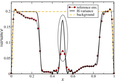
In Fig. 1 we present a specially designed example for the evolution model governed by the 1-D Burgers equation (for details see Sect. 4). The difference between the reference value of the variance (circles) and the inverse Hessian based value (bold solid line) can be clearly seen within the ellipse. The reference variance is obtained by a direct Monte Carlo simulation.

SinceR∗(u,0)¯ andH (u)¯ in Eq. (6) are linear operators and we assume that errorsξb andξoare unbiased and normally distributed, thenδu∼N(0,Vδu). Clearly, this result is valid

as far as the TLH and consequently Eq. (6) itself are satisfied. However, for highly nonlinear dynamical models the TLH often breaks down (e.g. Pires et al., 1996); thus, we have to

0 0.2 0.4 0.6 0.8 1

x

0 0.05 0.1 0.15 0.2

variance

reference ens. H-variance background

Fig. 1. Reference variance, variance by the inverse Hessian and

background variance.

SinceR∗

(¯u,0)and H(¯u)in (6) are linear operators and 160

we assume that errorsξb andξo are unbiased and normally

distributed, thenδu_{∼ N}(0,Vδu). Clearly, this result is valid

as far as the TLH and consequently (6) itself are satisfied. However, for highly nonlinear dynamical models the TLH often breaks down (e.g., Pires et al., 1996); thus, we have to 165

answer the following question: can the p.d.f. ofδustill be approximated by the normal distribution? If the answer is positive, one should look for a better approximation of the covariance than that given by (7).

Let us consider the cost function (2), but without the 170

background term. The corresponding error equation (5) is then as follows:

R∗

(¯u,δu)V−1

o R(¯u,τ δu)δu=R

∗

(¯u,δu)V−1

o ξo. (9)

For a univariate case, the classical result (see (Jennrich, 1969)) is that δu is asymptotically normal if ξo is an

175

independent identically distributed (i.i.d.) random variable withE[ξo] = 0andE[ξo2] =σ

2

<∞(’asymptotically’ means that T _{→ ∞} given the finite observation time step dt, or dt_→0 given the finite observation window [0,T]). Let us stress that for the asymptotic normality of δu the error 180

ξo is not required to be normal. This original result has

been generalized to the multivariate case and to the case of dependent, yet identically distributed observations (White and Domowitz, 1984), whereas an even more general case is considered in (Yuan and Jennrich, 1998). Here we 185

consider the complete cost function (2) and, correspondingly, the error equation (5), which contains terms related to the background term. To analyze a possible impact of these terms let us follow the reasoning in (Amemiya, 1983), pp. 337-345, where the error equation equivalent to (9) is 190

derived in a slightly different form. It is concluded that the errorδu is asymptotically normal when: a) the right-hand side of the error equation is normal; b) the left-right-hand side matrix converges in probability to a non-random value.

These conditions are met under certain general regularity 195

requirements to the operator R, which are incomparably weaker than the TLH and do not depend on the magnitude of the input errors. Clearly, as applied to (5), the first condition holds if ξb is normally distributed. SinceVb−1is

a constant matrix, the second condition always holds as long 200

as it holds forR∗

(¯u,δu)V−1

o R(¯u,τ δu). Therefore, one may

conclude thatδufrom (5) is bound to remain asymptotically normal. In practice the observation window[0,T]and time step dt are always finite implying the finite number of i.i.d. observations. Moreover, it is not easy to assess how 205

large the number of observations must be for the desired asymptotic properties to be reasonably approximated. Some nonlinear least-square problems in which the normality of the estimation error holds for ’practically relevant’ sample sizes are said to exhibit a ’close-to-linear’ statistical behavior 210

(Ratkowsky, 1983). The method suggested in (Ratkowsky, 1983) to verify this behavior is, essentially, a normality test applied to a generated sample of optimal solutions, which is hardly feasible for large-scale applications. Nevertheless, for certain highly nonlinear evolution models it is reasonable to 215

expect that the distribution ofδumight be reasonably close to normal if the number of i.i.d. observations is significant in time and the observation network is sufficiently dense in space. This may happen in assimilation of long time series of satellite observations of ocean surface elevation and 220

temperature, for example.

3 Effective Inverse Hessian (EIH) method

3.1 General consideration

Here we present a new method for estimating the covariance Vδu to be used in the case of highly nonlinear dynamics,

225

when[H(¯u)]−1

is not expected to be a good approximation of Vδu. Let us consider the discretized nonlinear error

equation (5) and denote byHthe left-hand side operator in (5). Then we can write down the expression forδu:

δu=_H−1 (V−1

b ξb+R

∗

(¯u,δu)V−1

o ξo),

230

whereas for the covarianceVδuwe obtain as follows:

Vδu:=EδuδuT=EH−1Vb−1ξbξbTV

−1

b H

−1∗ +

+E H−1

R∗

(¯u,δu)V−1

o ξoξoTV

−1

o R(¯u,δu)H

−1∗

. (10)

As a result of a series of simplifications described in (Gejadze et al., 2011) the above equation can be reduced to the form 235

Vδu≈V =E[H(¯u+δu)]−1, (11)

where H(¯u+δu) =V−1

b +R

∗

(¯u,δu)V−1

o R(¯u,δu) is the

Hessian of the linearized (auxiliary) control problem. The right-hand side of (11) may be called the effective inverse Hessian (EIH), hence the name of the suggested method.

Fig. 1. Reference variance, variance by the inverse Hessian and

background variance.

answer the following question: can the p.d.f. ofδustill be approximated by the normal distribution? If the answer is positive, one should look for a better approximation of the covariance than that given by Eq. (7).

Let us consider the cost function Eq. (2), but without the background term. The corresponding error equation Eq. (5) is then as follows:

R∗(u,δu)V¯ _o−1R(u,τ δu)δu¯ =R∗(u,δu)V¯ _o−1ξo. (9) For a univariate case, the classical result (see Jennrich, 1969) is thatδu is asymptotically normal ifξo is an independent identically distributed (i.i.d.) random variable withE[ξo] =0 andE[ξ_o2] =σ2<∞(“asymptotically” means thatT → ∞ given the finite observation time stepdt, ordt→0 given the finite observation window[0,T]). Let us stress that for the asymptotic normality ofδu, the errorξois not required to be normal. This original result has been generalized to the mul-tivariate case and to the case of dependent, yet identically dis-tributed observations (White and Domowitz, 1984), whereas an even more general case is considered in (Yuan and Jen-nrich, 1998). Here we consider the complete cost function Eq. (2) and, correspondingly, the error Eq. (5), which con-tains terms related to the background term. To analyze a possible impact of these terms let us follow the reasoning in (Amemiya, 1983), pp. 337–345, where the error equation equivalent to Eq. (9) is derived in a slightly different form. It is concluded that the error δu is asymptotically normal when: (a) the right-hand side of the error equation is nor-mal; (b) the left-hand side matrix converges in probability to a non-random value. These conditions are met under certain general regularity requirements to the operatorR, which are incomparably weaker than the TLH and do not depend on the magnitude of the input errors. Clearly, as applied to Eq. (5), the first condition holds ifξbis normally distributed. Since V_b−1is a constant matrix, the second condition always holds as long as it holds forR∗(u,δu)V¯ _o−1R(u,τ δu). Therefore,¯

one may conclude thatδufrom Eq. (5) is bound to remain asymptotically normal. In practice the observation window [0,T]and time stepdt are always finite implying the finite number of i.i.d. observations. Moreover, it is not easy to assess how large the number of observations must be for the desired asymptotic properties to be reasonably approx-imated. Some nonlinear least-square problems, in which the normality of the estimation error holds for “practically rele-vant” sample sizes, are said to exhibit a “close-to-linear” sta-tistical behavior (Ratkowsky, 1983). The method suggested in (Ratkowsky, 1983) to verify this behavior is, essentially, a normality test applied to a generated sample of optimal so-lutions, which is hardly feasible for large-scale applications. Nevertheless, for certain highly nonlinear evolution models, it is reasonable to expect that the distribution ofδu might be reasonably close to normal if the number of i.i.d. obser-vations is significant in time and the observation network is sufficiently dense in space. This may happen in assimilation of long time series of satellite observations of ocean surface elevation and temperature, for example.

3 Effective Inverse Hessian (EIH) method 3.1 General consideration

Here we present a new method for estimating the covari-anceVδuto be used in the case of highly nonlinear dynamics,

when[H (u)¯ ]−1is not expected to be a good approximation ofVδu. Let us consider the discretized nonlinear error

equa-tion Eq. (5) and denote byHthe left-hand side operator in Eq. (5). Then we can write down the expression forδu δu=H−1_(V−1

b ξb+R ∗

(u,δu)V¯ _o−1ξo),

whereas for the covarianceVδuwe obtain as follows:

Vδu:=E

h δuδuT

i =E

h

H−1_V−1 b ξbξ

T

b V −1 b H

−1∗i₊

+EhH−1_R∗_(u,δu)V¯ −1 o ξoξoTV

−1

o R(u,δu)¯ H

−1∗i_{. (10)} As a result of a series of simplifications described in (Gejadze et al., 2011) the above equation can be reduced to the form Vδu≈V=E

h

[H (u¯+δu)]−1i, (11)

whereH (u¯+δu)=V_b−1+R∗(u,δu)V¯ _o−1R(u,δu)¯ is the Hes-sian of the linearized (auxiliary) control problem. The right-hand side of Eq. (11) may be called the effective inverse Hes-sian (EIH), hence the name of the suggested method. In order to computeV directly using this equation, the expectation is substituted by the sample mean:

V= 1 L

L

X

l=1

180 V. Shutyaev et al.: Optimal solution error covariance

The main difficulty with the implementation is a need to compute a sample of optimal solutionsul= ¯u+δul.

How-ever, formula Eq. (11) does not necessarily requireul to be

an optimal solution. If we denote byqδuthe p.d.f. ofδu, then

equation Eq. (11) can be rewritten in the form: V=

Z +∞ −∞

[H (u¯+v)]−1qδu(v) dv. (13)

If we assume that in our nonlinear case the covariance matrix V describes meaningfully the p.d.f. of the optimal solution error, then, with the same level of validity, we should also accept the pdfqδuto be approximately normal with zero

ex-pectation and the covarianceV, in which case we obtain V=c

Z +∞ −∞

[H (u¯+v)]−1exp

−1 2v

T_V−1_v

dv, (14) wherec−1=(2π )M/2|V|1/2. Formula Eq. (12) givesV ex-plicitly, but requires a sample of optimal solutions ul, l=

1,...,Lto be computed. In contrast, the latest expression is a nonlinear matrix integral equation with respect toV, whilev is a dummy variable. This equation is actually solved using the iterative process Eq. (19), as explained in the following section. It is also interesting to notice that Eq. (14) is a deter-ministic equation.

3.2 Implementation remarks

Remark 1. Preconditioning is used in variational DA to ac-celerate the convergence of the conjugate gradient algorithm at the stage of inner iterations of the Gauss-Newton (GN) method, but it also can be used to accelerate formation of the inverse Hessian by the Lanczos algorithm (Fisher et al., 2009) or by the BFGS (Gejadze et al., 2010). SinceHis self-adjoint, we must consider a projected Hessian in a symmetric form

˜

H=(B−1)∗H B−1,

with some operatorB:X→X, defined in such a way that the eigenspectrum of the projected HessianH˜ is clustered around 1, i.e. the majority of the eigenvalues ofH˜ are equal or close to 1. Since the condition number ofH˜ is supposed to be much smaller than the condition number ofH, a sen-sible approximation ofH˜−1can usually be obtained (either by Lanczos or BFGS) with a relatively small number of iter-ations. After that, having_H˜−1_{, one can easily recoverH}−1 using the formula:

H−1=B−1H˜−1(B−1)∗. (15) Assuming that B−1does not depend on δul, we substitute

Eq. (15) into Eq. (12) and obtain the version of Eq. (12) with preconditioning:

V=B−1 1 L

L

X

l=1

[ ˜H (u¯+δu_l)]−1 !

(B−1)∗. (16)

Similarly, assuming thatB−1does not depend on the variable of integration, we substitute Eq. (15) into Eq. (14) and obtain the version of Eq. (14) with preconditioning:

V=B−1V (B˜ −1)∗,

˜ V=c

Z +∞ −∞

[ ˜H (u¯+v)]−1exp

−1 2v

T_V−1_v

dv. (17)

Formulas Eq. (16) and Eq. (17) instead ofH−1 involve ˜

H−1which is much less expensive to compute and store in memory. Let us mention here that the EIH method would hardly be feasible for large-scale problems without appropri-ate preconditioning.

Remark 2. The nonlinear Eq. (17) can be solved, for ex-ample, by the fixed point iterative process as follows Vp+1=B−1V (B˜ −1)∗,

˜ V=cp

Z +∞ −∞

[ ˜H (u¯+v)]−1exp

−1 2v

T_(Vp₎−1_v

dv, (18)

forp=0,1,..., starting with V0= [H (u)¯ ]−1. The iterative processes of this type are expected to converge if V0 is a good initial approximation of V, which is the case in the considered examples. The convergence of Eq. (18) and other methods for solving equation Eq. (17) are subjects for future research.

Remark 3. Different methods can be used for evaluation of the multidimensional integral in Eq. (18) such as quasi-Monte Carlo (Neiderreiter, 1992). Here, for simplicity, we use the standard Monte Carlo method. This actually implies a return to the formula Eq. (16). Taking into account Eq. (15), the iterative process takes the form

Vp+1=B−1 1 L

L

X

l=1

[ ˜H (u¯+δup

l )]

−1 !

(B−1)∗, (19)

whereδup

l ∼N(0,V

p_{). For eachl, we computeδu}p

l as

fol-lows δup

l =(V

p₎1/2_ξ

l,

whereξ∼N(0,I )is an independent random series,I is the identity matrix and(Vp)1/2is the square root ofVp. One can see that for eachpthe last formula looks similar to Eq. (16) with one key difference: δup_l in Eq. (19) is not an optimal solution, but a vector having the statistical properties of the optimal solution.

Remark 4. Let us notice that a few tens of outer iterations by the GN method may be required to obtain one optimal so-lution, while an approximate evaluation ofH˜−1is equivalent (in terms of computational costs) to just one outer iteration of the GN method. One has to repeat these computationsp times, however, only a few iterations on indexpare required in practice. Therefore, one should expect an order of the magnitude reduction of computational costs by the method

V. Shutyaev et al.: Optimal solution error covariance 181

Eq. (19) as compared to Eq. (16) for the same sample size. Clearly, for realistic large-scale models, the sample sizeLis going to be limited. Probably, the minimum ensemble size for this method to work is 2L∗+1, whereL∗is the accepted number of leading eigenvectors ofVpin Eq. (19).

Remark 5. In order to implement the process Eq. (19) a sample of vectorsϕl(x,0)=δup_l must be propagated from

t=0 tot=T using the nonlinear model Eq. (1). Therefore, for eachpone gets a sample of final statesϕl(x,T )consistent

with the current approximation ofVp, which can be used to evaluate the forecast and forecast covariance. SinceVp is a better approximation of the analysis error covariance than simply[H (u)¯ ]−1, one should expect a better quality of the forecast and covariance (as being consistent withVp, rather than with[H (u)¯ ]−1).

4 Numerical implementation 4.1 Numerical model

As a model we use the 1D Burgers equation with a nonlinear viscous term:

∂ϕ ∂t +

1 2

∂(ϕ2) ∂x = ∂ ∂x µ(ϕ)∂ϕ ∂x , (20)

ϕ=ϕ(x,t ), t∈(0,T ), x∈(0,1), with the Neumann boundary conditions

∂ϕ ∂x

x=0 =∂ϕ ∂x

x=1

=0 (21)

and the viscosity coefficient µ(ϕ)=µ0+µ1

_∂ϕ ∂x

2

, µ0,µ1=const >0. (22) The nonlinear diffusion term withµ(ϕ)dependent on∂ϕ/∂x is introduced to mimic the eddy viscosity (turbulence), which depends on the field gradients (pressure, temperature), rather than on the field value itself. This type ofµ(ϕ)also allows us to formally qualify the problem Eqs. (20)–(22) as strongly nonlinear (Fuˇcik and Kufner, 1980). Let us mention that the Burgers equations are sometimes considered in DA context as a simple model describing the atmospheric flow motion.

We use the implicit time discretization as follows ϕi−ϕi−1

ht

+ ∂ ∂x

₁ 2w(ϕ

i_)ϕi_−µ(ϕi₎∂ϕi

∂x

=0, (23)

wherei=1,...,N is the time integration index,ht=T /Nis

the time step. The spatial operator is discretized on a uniform grid (hxis the spatial discretization step,j=1,...,M is the

node number, M is the total number of grid nodes), using the “power law” first-order scheme as described in (Patankar, 1980), which yields quite a stable discretization scheme (this Remark 4. Let us notice that a few tens of outer iterations by the GN method may be required to obtain one 325

optimal solution, while an approximate evaluation ofH˜−1

is equivalent (in terms of computational costs) to just one outer iteration of the GN method. One has to repeat these computationsptimes, however only a few iterations on index pare required in practice. Therefore, one should expect an 330

order of the magnitude reduction of computational costs by the method (19) as compared to (16) for the same sample size. Clearly, for realistic large-scale models the sample size Lis going to be limited. Probably, the minimum ensemble size for this method to work is 2L∗

+ 1 , whereL∗

is the 335

accepted number of leading eigenvectors ofVp_{in (19).}

Remark 5. In order to implement the process (19) a sample of vectorsϕl(x,0) =δup_l must be propagated from

t= 0tot=T using the nonlinear model (1). Therefore, for eachpone gets a sample of final states ϕl(x,T)consistent

340

with the current approximation ofVp, which can be used to evaluate the forecast and forecast covariance. SinceVp _is

a better approximation of the analysis error covariance than simply[H(¯u)]−1

, one should expect a better quality of the forecast and covariance (as being consistent withVp_{, rather}

345

than with[H(¯u)]−1

).

4 Numerical implementation

4.1 Numerical model

As a model we use the 1D Burgers equation with a nonlinear viscous term: 350 ∂ϕ ∂t + 1 2

∂(ϕ2₎

∂x = ∂ ∂x

µ(ϕ)∂ϕ

∂x

, (20)

ϕ=ϕ(x,t), t_∈(0,T), x_∈(0,1),

with the Neumann boundary conditions ∂ϕ ∂x x=0 =∂ϕ ∂x x=1

= 0 (21)

and the viscosity coefficient 355

µ(ϕ) =µ0+µ1

∂ϕ ∂x

2

, µ0,µ1=const >0. (22)

The nonlinear diffusion term withµ(ϕ)dependent on∂ϕ/∂x is introduced to mimic the eddy viscosity (turbulence), which depends on the field gradients (pressure, temperature), rather than on the field value itself. This type ofµ(ϕ)also allows 360

us to formally qualify the problem (20)-(22) as strongly nonlinear (Fuˇcik and Kufner, 1980). Let us mention that the Burgers equations are sometimes considered in DA context as a simple model describing the atmospheric flow motion.

We use the implicit time discretization as follows: 365

ϕi_−ϕi−1

ht

+ ∂

∂x

₁

2w(ϕ

i_)ϕi_−µ(ϕi₎∂ϕi

∂x

= 0, (23)

ϕ

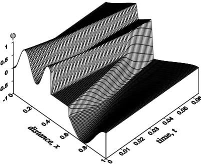
Fig. 2. Field evolution.

wherei= 1,...,N is the time integration index,ht=T /Nis

the time step. The spatial operator is discretized on a uniform grid (hxis the spatial discretization step,j= 1,...,M is the

node number,M is the total number of grid nodes) using 370

the ’power law’ first-order scheme as described in (Patankar, 1980), which yields quite a stable discretization scheme (this scheme allowsµ(ϕ) to be as small as0.5×10−4

for M= 200without noticeable oscillations). For each time step we perform nonlinear iterations on the coefficientsw(ϕ) =ϕ 375

andµ(ϕ)in the form ϕi

n−ϕin−1

ht

+ ∂

∂x

₁

2w(ϕ

i

n−1)ϕin−µ(ϕin−1)

∂ϕi n

∂x

= 0,

forn= 1,2,..., assuming initially thatµ(ϕi

0) =µ(ϕi −1₎

and w(ϕi0) =ϕi

−1

, and keep iterating until (23) is satisfied (i.e. the norm of the left-hand side in (23) becomes smaller than 380

the threshold ǫ1= 10−12 √

M). In all the computations presented in this paper we use the following parameters: the observation period T= 0.312, the discretization steps ht= 0.004,hx= 0.005, the state vector dimensionM= 200,

and the parameters in (22)µ0= 10−4,µ1= 10−6.

385

A general property of the Burgers solutions is that a smooth initial state evolves into a state characterized by the areas of severe gradients (or even shocks in the inviscid case). These are precisely the areas of a strong nonlinearity where one might expect violations of the TLH and, subsequently, 390

the invalidity of (7). For numerical experiments we choose a certain initial condition which stimulates the highly nonlinear behavior of the system; this is given by the formula

¯

u(x) =ϕ(x,0) =  



0.5₋0.5cos(8πx), 0_≤x_≤0.4,

0, 0.4< x_≤0.6

0.5cos(4πx)−0.5, 0.6< x≤1.

Fig. 2. Field evolution.

scheme allowsµ(ϕ)to be as small as 0.5×10−4for M= 200 without noticeable oscillations). For each time step we perform nonlinear iterations on the coefficientsw(ϕ)=ϕand µ(ϕ)in the form

ϕ_ni−ϕ_ni−1 ht + ∂ ∂x ₁ 2w(ϕ i

n−1)ϕni−µ(ϕni−1) ∂ϕi_n

∂x

=0, forn=1,2,..., assuming initially thatµ(ϕ₀i)=µ(ϕi−1)and w(ϕ₀i)=ϕi−1, and keep iterating until Eq. (23) is satisfied (i.e. the norm of the left-hand side in Eq. (23) becomes smaller than the threshold1=10−12√_{M). In all the} com-putations presented in this paper we use the following pa-rameters: the observation periodT =0.312, the discretiza-tion steps ht=0.004, hx=0.005, the state vector

dimen-sion M=200, and the parameters in Eq. (22) µ0=10−4, µ1=10−6.

A general property of the Burgers solutions is that a smooth initial state evolves into a state characterized by the areas of severe gradients (or even shocks in the inviscid case). These are precisely the areas of a strong nonlinearity where one might expect violations of the TLH and, subsequently, the invalidity of Eq. (7). For numerical experiments we choose a certain initial condition that stimulates the highly nonlinear behavior of the system; this is given by the for-mula:

¯

u(x)=ϕ(x,0)=   

0.5−0.5cos(8π x), 0≤x≤0.4, 0, 0.4< x≤0.6

0.5cos(4π x)−0.5, 0.6< x≤1. The resulting field evolutionϕ(x,t )is presented in Fig. 2. 4.2 BFGS for computing the inverse Hessian and

other details

182 V. Shutyaev et al.: Optimal solution error covariance

6 V. Shutyaev et al.: Optimal solution error covariance

The resulting field evolutionϕ(x,t)is presented in Fig.2. 395

4.2 BFGS for computing the inverse Hessian and other details

The projected inverse Hessian H˜(¯u+δu) is computed as a collateral result of the BFGS iterations while solving the following auxiliary DA problem:

400

  

 

∂δϕ ∂t −F

′

(ϕ)δϕ= 0, t∈(0,T)

δϕ

t=0 =B −1_δu

J1(δu) = inf

v J1(v),

(24)

where

J1(δu) = 1 2(V

−1

b B

−1

(δu₋ξb),B−1(δu−ξb))X+

+1 2(V

−1

o (Cδϕ−ξo),Cδϕ−ξo)Yo. (25)

The preconditioner used in our method is 405

B−1

=V_b1/2[ ˜H(¯u)]−1/2

. (26)

In order to compute [ ˜H(¯u)]−1_/2

we apply the Cholesky factorization of the explicitly formed matrix H˜−1

. However, it is important to note that the square-root-vector productH˜−1/2

wcan be computed using a recursive 410

procedure based on the accumulated secant pairs (BFGS) or eigenvalues/eigenvectors (Lanczos) as described in (Tshimanga et al., 2008), without the need to formH˜−1

and to factorize it. Consistent tangent linear and adjoint models have been generated from the original forward model by 415

the Automatic Differentiation tool TAPENADE (Hasco¨et and Pascual, 2004) and checked using the standard gradient test. The background error covariance Vb is computed

assuming that the background error belongs to the Sobolev space W2

2[0,1](see Gejadze et al., 2010, for details). The

420

correlation function used in the numerical examples is as presented in Fig.3, the background error variance is σ2

b= 0.2, the observation error variance isσ

2

o= 10

−3

. The observation scheme consists of 4 sensors located at the points xˆk = 0.4,0.45,0.55,0.6, and the observations are

425

available at each time instant.

5 Numerical results

First we compute a large sample (L= 2500) of optimal solutionsulby solvingLtimes the data assimilation problem

(1)-(2) with perturbed data ub= ¯u+ξb and y=Cϕ¯+ξo,

430

whereξb∼ N(0,Vb)andξo∼ N 0,σo2I

. This large sample is used to evaluate the sample covariance matrix, which is further processed to filter the sampling error (as described in Gejadze et al., 2011); the outcome is considered as a reference value Vˆ◦

. Then, the original large sample 435

is partitioned into one hundred subsets including L= 25

-0.3 -0.2 -0.1 0 0.1 0.2 0.3

x 0

0.2 0.4 0.6 0.8 1

correlation

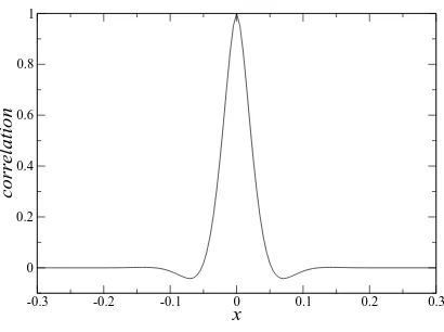
Fig. 3. Correlation function.

members and into twenty five subsets including L= 100

members. Let us denote byVˆLthe sample covariance matrix

obtained for a subset including L members. Then, the relative error in the sample variance (which is the relative 440

sampling error) can be defined as the vector ˆεL with the

components

(ˆεL)i= ( ˆVL)i,i/Vˆi,i◦−1, i= 1,...,M.

The relative error in a certain approximation ofV is defined as a vectorεwith the components

445

εi=Vi,i/Vˆi,i◦−1, i= 1,...,M. (27)

We compute this error withV in (27) being estimated by one of the following methods:

1) by the inverse Hessian method, i.e. simply usingVδu=

[H(¯u)]−1

; 450

2a) by the EIH method implemented in the form (16), which requires a sample of optimal solutionsδulto be computed;

2b) by the EIH method implemented as the iterative process (19), which requires a sample of δul, but does not require

thatδulare optimal solutions.

455

For the computation ofV by the methods 2a or 2b a sample ofδul is required, hence the result depends on the sample

size L. The results (obtained by the methods 2a and 2b) presented in this paper are computed withL= 100. In the method 2b we currently allow enough iterations on the index 460

pfor the iterative process (19) to converge in terms of the distance between the successive iterates. In practice, this requires just a few iterations, typically2₋3.

In the upper panel in Fig.4 a set of one hundred vectors

ˆ

ε25is presented in dark lines, and a set of twenty five vectors

465

ˆ

ε100 - in the overlaying white lines. These plots reveal

the envelopes for the relative error in the sample variance obtained withL= 25andL= 100, respectively. The graphs ofεare presented in the lower panel: line 1 corresponds to the method 1 (the inverse Hessian method, see also Fig.1), 470

lines 2 and 3 - to the methods 2a and 2b (variants of the EIH method).

Fig. 3. Correlation function.

following auxiliary DA problem: 

   

∂δϕ ∂t −F

0_{(ϕ)δϕ=0, t∈(0,T )} δϕ

t=0=B −1_δu J1(δu)=inf

v J1(v),

(24)

where J1(δu)=

1 2(V

−1 b B

−1_(δu−ξ

b),B−1(δu−ξb))X+

+1 2(V

−1

o (Cδϕ−ξo),Cδϕ−ξo)Yo. (25)

The preconditioner used in our method is

B−1=V_b1/2[ ˜H (u)¯ ]−1/2. (26) In order to compute [ ˜H (u)¯ ]−1/2 we apply the Cholesky factorization of the explicitly formed matrix H˜−1. How-ever, it is important to note that the square-root-vector prod-uct H˜−1/2w can be computed using a recursive procedure based on the accumulated secant pairs (BFGS) or eigenval-ues/eigenvectors (Lanczos) as described in (Tshimanga et al., 2008), without the need to formH˜−1and to factorize it. Con-sistent tangent linear and adjoint models have been generated from the original forward model by the Automatic Differ-entiation tool TAPENADE (Hasco¨et and Pascual, 2004) and checked using the standard gradient test. The background er-ror covarianceVbis computed assuming that the background error belongs to the Sobolev spaceW₂2[0,1](see Gejadze et al., 2010, for details). The correlation function used in the numerical examples is as presented in Fig. 3, the background error variance isσ_b2=0.2, the observation error variance is σ_o2=10−3. The observation scheme consists of 4 sensors located at the pointsxˆk=0.4,0.45,0.55,0.6, and the

obser-vations are available at each time instant.

5 Numerical results

First we computed a large sample (L=2500) of optimal so-lutionsul by solvingLtimes the data assimilation problem

Eqs. (1)–(2) with perturbed dataub= ¯u+ξbandy=Cϕ¯+ξo, whereξb∼N(0,Vb)andξo∼N 0,σo2I

. This large sample was used to evaluate the sample covariance matrix, which was further processed to filter the sampling error (as de-scribed in Gejadze et al., 2011); the outcome was considered as a reference valueVˆ◦. Then, the original large sample was partitioned into one hundred subsets includingL=25 mem-bers and into twenty five subsets includingL=100 members. Let us denote byVˆLthe sample covariance matrix obtained

for a subset includingLmembers. Then, the relative error in the sample variance (which is the relative sampling error) can be defined as the vectorεˆLwith the components:

(εˆL)i=(VˆL)i,i/Vˆi,i◦−1, i=1,...,M.

The relative error in a certain approximation ofV is defined as a vectorεwith the components:

εi=Vi,i/Vˆi,i◦ −1, i=1,...,M. (27)

We compute this error withV in Eq. (27) being estimated by one of the following methods:

1. by the inverse Hessian method, i.e. simply using Vδu= [H (u)¯ ]−1;

2a. by the EIH method implemented in the form Eq. (16), which requires a sample of optimal solutionsδul to be

computed;

2b. by the EIH method implemented as the iterative process Eq. (19), which requires a sample ofδul, but does not

require thatδul are optimal solutions.

For the computation ofV by the methods 2a or 2b a sample ofδul is required, hence, the result depends on the sample

size L. The results (obtained by the methods 2a and 2b) presented in this paper are computed withL=100. In the method 2b we currently allow enough iterations on the index p for the iterative process Eq. (19) to converge in terms of the distance between the successive iterates. In practice, this requires just a few iterations, typically 2−3.

In the upper panel in Fig. 4, a set of one hundred vectors ˆ

ε25 is presented in dark lines, and a set of twenty five vec-torsεˆ100- in the overlaying white lines. These plots reveal the envelopes for the relative error in the sample variance ob-tained with L=25 andL=100, respectively. The graphs ofεare presented in the lower panel: line 1 corresponds to the method 1 (the inverse Hessian method, see also Fig. 1), lines 2 and 3 – to the methods 2a and 2b (variants of the EIH method).

0.1 0.2 0.3 0.4 0.5 0.6 0.7 0.8 0.9

x

-0.5 0 0.5 1

ε^

0.1 0.2 0.3 0.4 0.5 0.6 0.7 0.8 0.9

x

-0.5 0 0.5 1

ε

1 2 3

Fig. 4. Up: the sample relative error εˆ_{. Set of}εˆ_forL= 25

-dark envelope and set ofεˆ_forL= 100_{- white envelope. Down:}

the relative errorε_{by the inverse Hessian - line 1, and by the EIH} methods withL= 100: method 2a - line 2; method 2b - line 3.

Looking at Fig.4 we observe that the relative error in the sample variance εˆ25 (dark envelope) exceeds 50%almost everywhere, which is certainly beyond reasonable margins,

475

andεˆ100 (white envelope) is around25%(that is still fairly large). In order to reduce the white envelope two times, one would need to use the sample size L= 400, etc. One should also keep in mind that the relative error in the diagonal elements of the sample covariance matrix is the smallest

480

as compared to its sub-diagonals, i.e. the envelopes for any sub-diagonal would be wider than those presented in Fig.4(up). Thus, the development of methods for estimating the covariance (alternative to the direct sampling method) is an important task.

485

Whereas the method 1 (the inverse Hessian method) gives an estimate ofVδuwith a small relative error (as compared to

the sample covariance) in the areas of mild nonlinearity, this error can be much larger in the areas of high nonlinearity. For example, if we imagine that the lower panel in Fig.4 is

490

superposed over its upper panel, then one could observe line 1 jumping outside the dark envelope in the area surrounding

x= 0.5, i.e. the relative error by the inverse Hessian is significantly larger here than the sampling error for L=

25. At the same time, the relative error obtained by the

495

methods 2a and 2b is much smaller as compared to the error in line 1 and it would largely remain within the white envelope. The difference between the estimates by the methods 2a and 2b does not look significant. The best improvement can be achieved for the diagonal elements of

500

Vδu (the variance). Thus, the covariance estimate by the

EIH method is noticeably better than the sample covariance obtained with the equivalent sample size. The suggested algorithm is computationally efficient (in terms of the CPU time) if the cost of computing the inverse Hessian is much

505

less than the cost of computing one optimal solution. In the example presented in this paper one limited-memory inverse Hessian is about 20-30 times less expensive than one optimal solution. Thus, on average, the algorithm 2b works about 10 times faster than the algorithm 2a, whereas the results by

510

both the algorithms are similar in terms of accuracy.

6 Conclusions

Error propagation is a key point in modeling the large-scale geophysical flows, with the main difficulty being linked to the nonlinearity of the governing equations. In this paper

515

we consider the hind-cast (initialization) DA problem. From the mathematical point of view, this is the initial-value control problem for a nonlinear evolution model governed by partial differential equations. Assuming the so-called tangent linear hypothesis (TLH) holds, the covariance is

520

often approximated by the inverse Hessian of the objective function. In practice, the same approximation could be valid even though the TLH is clearly violated. However, here we deal with such a highly nonlinear dynamics that the inverse Hessian approach is no longer valid. In this case

525

a new method for computing the covariance matrix named the ’effective inverse Hessian’ method can be used. This method yields a significant improvement in the covariance estimate as compared to the inverse Hessian. The method is potentially feasible for large-scale applications because it

530

can be used in a multiprocessor environment and operates in terms of the Hessian-vector products. The software blocks needed for its implementation are the standard blocks of any existing 4D Var system. All the results of this paper are consistent with the assumption of a ’close-to-normal’

535

nature of the optimal solution error. This should be expected taking into account the consistency and asymptotic normality of the estimator and the fact that the observation window in variational DA is usually quite large. In this case the covariance matrix is a meaningful representative of the

540

p.d.f. The method suggested may become a valuable option for uncertainty analysis in the framework of the classical 4D-VAR approach when applied to highly nonlinear DA problems.

Acknowledgements. The first author acknowledges the Russian

545

Foundation for Basic Research and Russian Federal Research

Fig. 4. Up: the sample relative errorεˆ. Set ofεˆ forL=25 - dark envelope and set ofεˆforL=100 - white envelope. Down: the rela-tive errorεby the inverse Hessian - line 1, and by the EIH methods withL=100: method 2a - line 2; method 2b - line 3.

Looking at Fig. 4, we observe that the relative error in the sample varianceε25ˆ (dark envelope) exceeds 50% almost everywhere, which is certainly beyond reasonable margins, andεˆ100(white envelope) is around 25% (that is still fairly large). In order to reduce the white envelope two times, one would need to use the sample sizeL=400, etc. One should also keep in mind that the relative error in the diagonal el-ements of the sample covariance matrix is the smallest as compared to its diagonals, i.e. the envelopes for any sub-diagonal would be wider than those presented in Fig.4(up). Thus, the development of methods for estimating the covari-ance (alternative to the direct sampling method) is an impor-tant task.

Whereas the method 1 (the inverse Hessian method) gives an estimate ofVδuwith a small relative error (as compared to

the sample covariance) in the areas of mild nonlinearity, this error can be much larger in the areas of high nonlinearity. For example, if we imagine that the lower panel in Fig. 4 is superposed over its upper panel, then one could observe line 1 jumping outside the dark envelope in the area surround-ingx=0.5, i.e. the relative error by the inverse Hessian is significantly larger here than the sampling error forL=25.

At the same time, the relative error obtained by the meth-ods 2a and 2b is much smaller as compared to the error in line 1 and it would largely remain within the white enve-lope. The difference between the estimates by the methods 2a and 2b does not look significant. The best improvement can be achieved for the diagonal elements ofVδu(the

vari-ance). Thus, the covariance estimate by the EIH method is noticeably better than the sample covariance obtained with the equivalent sample size. The suggested algorithm is com-putationally efficient (in terms of the CPU time) if the cost of computing the inverse Hessian is much less than the cost of computing one optimal solution. In the example presented in this paper one limited-memory inverse Hessian is about 20– 30 times less expensive than one optimal solution. Thus, on average, the algorithm 2b works about 10 times faster than the algorithm 2a, whereas the results by both the algorithms are similar in terms of accuracy.

6 Conclusions

184 V. Shutyaev et al.: Optimal solution error covariance

Acknowledgements. The first author acknowledges the Russian

Foundation for Basic Research and Russian Federal Research Program “Kadry”. The second author acknowledges the funding through the Glasgow Research Partnership in Engineering by the Scottish Funding Council. All the authors thank the editor and the anonymous reviewers for their useful comments and suggestions.

Edited by: O. Talagrand

Reviewed by: three anonymous referees

References

Amemiya, T.: Handbook of econometrics, 1, North-Holland Pub-lishing Company, Amsterdam, 1983.

Courtier, P., Th´epaut, J. N., and Hollingsworth, A.: A strategy for operational implementation of 4D-Var, using an incremental ap-proach, Q. J. Roy. Meteor. Soc., 120, 1367–1388, 1994. Draper, N.R., Smith, H.: Applied regression analysis, 2nd ed.,

Wi-ley, New York, 1981.

Fisher, M., Nocedal, J., Tr´emolet, Y., and Wright, S. J.: Data assim-ilation in weather forecasting: a case study in PDE-constrained optimization, Optim. Eng., 10, 409–426, 2009.

Fuˇcik, S. and Kufner, A.: Nonlinear differential equations, Elsevier, Amsterdam, 1980.

Gejadze, I., Le Dimet, F.-X., and Shutyaev, V.: On analysis error co-variances in variational data assimilation, SIAM J. Sci. Comput., 30, 1847–1874, 2008.

Gejadze, I., Le Dimet, F.-X., and Shutyaev, V.: On optimal solu-tion error covariances in variasolu-tional data assimilasolu-tion problems, J. Comput. Phys., 229, 2159–2178, 2010.

Gejadze, I. Yu., Copeland, G. J. M., Le Dimet, F.-X., and Shutyaev, V.: Computation of the analysis error covariance in variational data assimilation problems with nonlinear dynamics, J. Comput. Phys., 230, 7923–7943, 2011.

Hasco¨et, L., Pascual, V.: TAPENADE 2.1 user’s guide, INRIA Technical Report 0300, 78 pp., 2004.

Jennrich, R. I.: Asymptotic properties of nonlinear least square es-timation, Ann. Math. Stat., 40, 633–643, 1969.

Le Dimet, F. X. and Talagrand, O.: Variational algorithms for anal-ysis and assimilation of meteorological observations: theoretical aspects, Tellus, 38A, 97–110, 1986.

Lions, J. L.: Contrˆole optimal des syst`emes gouvern´es par des ´equations aux d´eriv´ees partielles, Dunod, Paris, 1986.

Liu, D. C. and Nocedal, J.: On the limited memory BFGS method for large scale minimization, Math. Program., 45, 503–528, 1989.

Marchuk, G. I., Agoshkov, V. I., and Shutyaev, V. P.: Adjoint equa-tions and perturbation algorithms in nonlinear problems, CRC Press Inc., New York, 1996.

Neiderreiter, H.: Random number generation and quasi-Monte Carlo methods, CBMS-NSF Regional Conference Series in Ap-plied Math., 63, SIAM, Philadelphia, 1992.

Patankar, S. V.: Numerical heat transfer and fluid flow, Hemisphere Publishing Corporation, New York, 1980.

Pires, C., Vautard, R., and Talagrand, O.: On extending the limits of variational assimilation in nonlinear chaotic systems, Tellus, 48A, 96–121, 1996.

Rabier, F. and Courtier, P.: Four-dimensional assimilation in the presence of baroclinic instability, Q. J. Roy. Meteor. Soc., 118, 649–672, 1992.

Ratkowsky, D. A.: Nonlinear regression modelling: a unified prac-tical approach, Marcel Dekker, New York, 1983.

Thacker, W. C.: The role of the Hessian matrix in fitting models to measurements, J. Geophys. Res., 94, 6177–6196, 1989. Tshimanga, J., Gratton, S., Weaver, A. T., and Sartenaer, A.:

Limited-memory preconditioners, with application to incremen-tal four-dimensional variational assimilation, Q. J. Roy. Meteor. Soc., 134, 751–769, 2008.

White, H. and Domowitz, I.: Nonlinear regression and dependent observations, Econometrica, 52/1, 143–162, 1984.

Yuan, K.-H. and Jennrich, R. I.: Asymptotics of estimating equa-tions under natural condiequa-tions, J. Multivariate Anal., 65, 245– 260, 1998.