INVESTIGATION OF THE EFFECT OF TRAFFIC PARAMETERS
ON ROAD HAZARD USING CLASSIFICATION TREE MODEL
Md. Mahmud Hasan1
1 School of Civil, Environmental and Chemical Engineering, RMIT University, Melbourne 3001, Australia
Received 1 May 2012; accepted 3 July 2012
Abstract: This paper presents a method for the identification of hazardous situations on the freeways. For this study, about 18 km long section of Eastern Freeway in Melbourne, Australia was selected as a test bed. Three categories of data i.e. traffic, weather and accident record data were used for the analysis and modelling. In developing the crash risk probability model, classification tree based model was developed in this study. In formulating the models, it was found that weather conditions did not have significant impact on accident occurrence so the classification tree was built using two traffic indices; traffic flow and vehicle speed only. The formulated classification tree is able to identify the possible hazard and non-hazard situations on freeway. The outcome of the study will aid the hazard mitigation strategies.
Keywords: road hazard, traffic parameter, classification tree, crash risk model, accident, decision tree.
1. Introduction
1 Corresponding author: [email protected]
Traffic performance indicators such as traffic flow and speed which can act as a proxy for the traffic condition may indicate hazardous situations leading to accidents. Weather conditions may also lead to situations which might hamper usual traffic movements and roadway safety. Adverse weather conditions not only reduce drivers’ visibility but also make the roads dangerous because of reduced friction between tyres and road surfaces (Goodwin, 2002). Road accident also induces traffic congestion. Due to accident, some or all the lanes of the roadway are blocked and vehicles are stuck in congestion for long durations. This congestion results in increased travel time, vehicle emissions and fuel usage etc. (Golob et al., 2004).
This study investigates the relationship among traffic parameters, weather and road hazards. Traffic flow and speed are the two important indices used to quantify the traffic performance while number of accident is used as a performance index for roadway safety. In the study, rainfall intensity is considered as the proxy of adverse weather condition. Statistical analysis method, regression tree, is used to evaluate how traffic parameters and rainfall influence road hazard occurrence.
5 and then in section 6, the process of model formulation is described thoroughly. The rest of the sections represent results, discussion and conclusion.
2. Literature Review
2.1. Traffic Flow and Road Accidents
A number of studies have been conducted to relate traffic flow with road crash propensity. Jean-Louis (2002) showed that damage-only and injury-involved incident rates are higher in light traffic than in heavy traffic conditions. He also compared the incident rates on the basis of time of the day and found that these rates do not depend on day time or night-time traffic. Hasan et al. (2011) have found that road accident probability on the freeway depends significantly on the traffic flow. They developed a regression tree by using traffic flow and speed at accident location, nearest upstream and downstream and concluded that road accidents depend more on traffic parameters: traffic flow and vehicle speed rather than weather condition.
On the contrary, Lord et al. (2005) showed that the crash risk cannot be predicted perfectly only by traffic flow but adding traffic density so improves the prediction performance. Furthermore, they also described the comparative difference of crash-density relationship between urban and rural freeways. For the same flow and density, it has been found that crash rates are much higher on urban freeways than the rural ones. Dickerson et al. (1998) revealed significant differences in accident - traffic flow relationship by road class and geography. Their outcomes are based on all types of accidents regardless of severity level. Accident probability also depends on type of vehicles (Ayati and Abbasi,
2011). Non-passenger car vehicles are found to cause more accidents on urban highways than other vehicle types. Interestingly, it was shown that heavy vehicles cause less accident than non-passenger cars including taxis and motorcycles.
2.2. Vehicle Speed and Road Accidents
Aarts et al. (2006) reviewed the literature on vehicle speed and road accident relationship and showed that road incidents increase significantly with an increase in speed on minor roads than on major roads. Similarly, Navon (2003) mentioned that excessive speed causes road crashes. He also described that the relationship between average speed and accident is not clear. Elvik (2004) described that mean speed is positively related with frequency and severity of accidents since the number of road accidents increases with increase of speed. In order to develop the relationship between speed and safety, Aljanahi et al. (1999) found significant positive relationship between mean speed and accident rate. Similarly, Hasan et al. (2011) also concluded that vehicle speed is a contributing factor to accidents’ occurrence on freeway. Also, Taylor et al. (2000) discussed the results of driver based and road based previous studies, and mentioned that higher speed causes more accidents. The outcome of the study showed that approximately 1 km/h decrease in average speed can reduce accident occurrence rate by 2% - 7%.
of accident rate is not so clear. While aiming to assess the effects of traffic congestion on the frequency of crash rate by using spatial analysis approach, Wang et al. (2009) found that traffic congestion has no impact on the frequency of accident occurrence (either for fatal crash or slight injury crash).
2.3. Accident Prediction Models
Mustakim et al. (2008) proposed an accident prediction model based on the dataset of Federal Route 50 in Malaysia. In this study, they considered number of access point per kilometre of the roadway, hourly traffic volume, time gap between vehicle and 85th percentile speed. Multiple linear regression model resulted in good accuracy level. Similarly, Hong et al. (2005) also used multiple regression methods in order to develop a crash prediction model but they focused more on road geometry compared to traffic conditions in choosing the independent variables. Road geometry was also considered as predictors in accident prediction model by Kalokota and Seneviratne (1994) but the selected geometry variables are different. Hong et al. (2005) chose number of intersections, connecting roads, pedestrian traffic signals, existence of median barrier and lanes, whereas Kalokota and Seneviratne (1994) selected degree of curvature, section length, vertical grade, number of lane, right shoulder width and traffic volume as predictors. This may be due to different site locations i.e. urban and rural highways.
Eisenberg (2004) has developed a crash risk prediction model based on weather variables such as precipitation and snowfall. Negative binomial regression method was used in this study and accident frequencies were predicted in terms of fatality, injury and
model has more accuracy than that by BP neural network.
3. Test Bed
The selected site for this study, Eastern Freeway in Melbourne (Australia) is one of the important urban freeways for commuting to city from eastern suburbs of Melbourne. The section for the study is approximately 18 km long, from Hoddle Street to Springvale road, consisting of three to five lanes in each direction. Between entry and exit points of the freeway, there are 7 off-ramps and 8 on-ramps in inbound direction and there are 8 off-ramps and 8 on-ramps in the outbound direction. The total roadway section is equipped with 65 detectors in which 32 detectors are located in outbound direction while the remaining 33 detectors are located in inbound direction.
4. Data Collection and Fusion
Three types of data are required in this study. These are: traffic data, accident data and weather data. Traffic flow and vehicle speed are considered as traffic performance indicator in this study. In case of accident data, detailed information for each of the road incidents including location, time, and severity is required for this study. Rainfall intensity data are also needed in this study to investigate the impact of rainfall on accidents. The required data used in this study are collected from two different organisations that provide Traffic data. Namely, VicRoads, which is the road authority of Victoria (Australia), collects data from the loop detectors on the selected roadway. VicRoads also provided detailed road accident information. Bureau of Meteorology (Australia) is responsible for collecting rainfall data from three weather
stations near the selected roadway. These three weather stations are View bank (Apsana), Scoresby Research Institute and Melbourne regional office. Traffic, rainfall and accidents data used in this study are from September 2007 till June 2010 which is approximately three years.
The minute-by-minute traffic data is aggregated to 5 minutes intervals, rainfall intensity data are being kept as hourly data and categorical crash data with specific crash time and locations are used for the analysis. Categorical crash data are set as a binary variable such as: Accident = ‘yes’, if there was an accident or Accident = ‘no’, if there was no accident at the given time and location. These three data types are used to prepare an aggregated database of 5 minute interval including date, hour, minute, detector location, traffic flow, speed and rainfall intensity during the hour and accident. Data fusion module was developed using programming language Perl.
5. Model Selection
In general, the dependency of the variables in the classification tree can be shown as Eq. (1):
Where, Y is the target variable (dependent variable) and x1, x2, x3,..., xn are predictor
variables (independent variables).
5.1. Building the Classification Tree
In this study, statistical software R is used to develop classification tree by recursive partitioning routine. Recursive partitioning is an exploratory technique to uncover the structure in data. It forms the base for nonparametric regression analysis: Classification and Regression Trees (CART). Model based on this method is built by splitting of dataset into increasing homogenous subsets until become infeasible to continue (Higgs and Cummings, 2003). The process of building the classification tree consists of the following steps:
Step 1: A single predictor variable is chosen for splitting. The predictor variable which can divide total dataset into two parts is selected for first splitting of the tree.
Step 2: The data is separated into two groups based on the chosen split.
Step3: This process is continued for each subgroup unless it reaches a previously defined minimum size, or until no improvement can be made (Therneau and Atkinson, 1997).
5.2. Splitting Criteria
According to Therneau and Atkinson (1997), if node A is to be split into two branches
named left son AL and right son AR, it needs to satisfy the following Eq. (2):
Where:
P(A) = probability of A I(A) = risk of A
P(AL) = probability of left son I(AL) = risk of left son
P(AR) = probability of right son I(AR) = risk of right son
The split which maximizes the ΔI i.e. decrease the risk, is chosen for building the tree (Eq. (3)):
Here (Eq. (4)):
where:
τ (A) = The class method of A, if A were to be taken as a final node.
πi = prior probabilities of each class; i = 1, 2,..., n L (i, j) = Loss matrix for incorrectly classifying an i as a j. i = 1, 2,..., C; L (i, i) = 0
ni, nA = number of observations in the sample that are in class i, number of observations in node A.
niA = number of observations in the sample that are in class i and node A. (Therneau and Atkinson, 1997)
(1) (2)
(3)
6. Model Formulation
6.1. Selection of Model Variables
6.1.1. Dependent Variable
As this classification tree model predicts the hazard occurrence, hazardous situation is considered as the dependent variable where categorical hazard value is either ‘Yes (1)’ or ‘No (0)’. ‘Yes (1)’ represents hazard condition and ‘No (0)’ represents non-hazard condition.
6.1.2. Independent Variables
Initially, thirteen independent variables are selected as predictor variables. Traffic flow, vehicle speed and rainfall intensity are considered independent variables in this model. Traffic flow and speed at current time, 5 minutes before, and 10 minutes before at the current detector location and at the nearest upstream detector location are used as independent variables for the modeling purpose. Corresponding rainfall intensity at the same time and location is also used as a predictor variable. To identify variables, q is taken as traffic flow (veh/min), v is taken as vehicle speed (km/h), l is chosen for location and t is chosen for time. Following is a list of variables used in the model:
q
l,t= Flow at the current location at currenttime
υ
l,t= Speed at the current location at currenttime
q
u,t = Flow at the nearest upstream of thecurrent location at current time
υ
u,t = Speed at upstream of the currentlocation at current time
q
l,t-5 = Flow at current location at 5 minutesbefore current time
υ
l,t-5 = Speed at current location at 5 minutesbefore current time
q
u,t-5 = Flow at nearest upstream of thecurrent location at 5 minutes before current time
υ
u,t-5 = Speed at nearest upstream of thecurrent location at 5 minutes before current time
q
l,t-10 = Flow at current location at 10minutes before current time
υ
l,t-10 = Speed at current location at 10minutes before current time
q
u,t-10 = Flow at nearest upstream of thecurrent accident location at 10 minutes before current time
υ
u,t-10 = Speed at nearest upstream of thecurrent location at 10 minutes before current time
Ri = Rainfall intensity
At first, all the variables are input in the software R to build the classification tree but it is found that the following predictors do not have significant contributions in classification tree building:
• Flow at current location at 5 minutes before current time,
q
l,t-5• Flow at current location at 10 minutes before current time,
q
l,t-10For the first two variables, the main reason was missing data. Compared to other predictors, these two variables have a number of missing data points. Although, there were no missing values in rainfall data but it is observed that only approximately 7% of dataset have hazard cases during rainy conditions which are insignificant compared to non-hazard cases and hence makes the use of rainfall intensity in crash hazard prediction trivial. For this reason, rainfall intensity, Ri is not taken into consideration by Rpart routine for tree building.
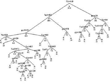
6.2. Building of Classification Tree Model
The classification tree is built by assuming that the minimum number of observations
in a terminal node is two and the minimum number of observations in a node for splitting is three. The tree consists of 54 nodes including 28 terminal nodes. The nodes are grown by meeting the criterion of specific range of predictor variables. If any observation meets the criterion, then it moves towards the left side, otherwise it moves to the right. Each node shows the hazard class “yes” or “no” along with the number of progression and non-progressions. The terminal nodes show the hazard and non-hazard occurrence condition by showing ‘yes’ (hazardous situation) or ‘no’ (non-hazardous situation). Total classification tree is shown in Fig. 1. It is observed from the classification tree that the most important variable for hazard
Fig. 1.
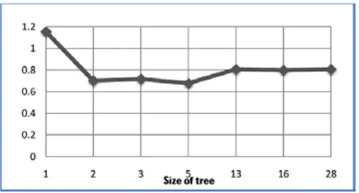
To find out the best classification tree for this analysis 1-SE rule is used which can calculate how many splits of the tree provide good results. In this rule, the split which has minimum value of cross-validation error and minimum value of (cross- validation error + cross-validation standard deviation) is considered as the best tree (Therneau and Atkinson, 1997). According to the 1-SE rule, by four splitting of the tree, the given result is
accurate e.g. the prediction of accidents is not over-fitted as this split has minimum value of cross-validation error along with the minimum value of cross validated standard deviation. The following diagram (Fig. 2), cross-validation error vs. size of tree (number of splits +1) depicts the same results as in above table. It is observed that with increasing number of splits of the tree the prediction is speed since most of the terminal
nodes and split points depend on it. If the predictors are evaluated by time and location, it is seen that the speed and flow at the time and location of the accident occurrence have more contribution to predict crash hazard.
6.3. Cross-Validation Result
Table 1 shows up to which split the tree can provide accurate results and indicates the best tree for this analysis. The table describes the scaled complexity parameter (cp), relative error (1-R2), cross validation error and cross validation standard deviation value of each split of tree, starting from 0 to 27 splits. Cross validation error is related to the PRESS ( Predicted Residual Sums of squares) statistics which is used to provide a summary measure of the fit of a model to a sample of
observations and it is calculated as the sum of all resulting errors (Therneau and Atkinson, 1997). The complexity parameter, cp is an advisory parameter and it is specified by the following formula (Eq. (6)):
Where, T0 is the tree with no splits and |T| is the number of terminal node. A value of cp = 1 will result in a tree with no splits. Scaled cp provides direct interpretation in regression model. For example: if any split does not improve the overall R2 of the model by at least
cp, the split is not branched further (Therneau and Atkinson, 1997). The following table depicts that within four splits of the tree, the cross-validation error is minimum while it increases with the addition of number of splits.
cp No. of split Relative error Cross-validationerror Cross-validated std.deviation
0.347 0 1.000 1.153 0.063
0.057 1 0.653 0.701 0.060
0.036 2 0.596 0.717 0.061
0.016 4 0.524 0.677 0.060
0.013 12 0.395 0.806 0.062
0.011 15 0.355 0.798 0.062
0.010 27 0.169 0.806 0.062
Table 1
CP Table (Errors in Each Split)
Fig. 2.
Cross-Validation Error vs. Size of the Tree
Fig. 3.
cross-validation error decreases, whereas after four splits (tree size = 5), the cross-validation error increases with the increase in the tree splits. So, instead of the whole tree, it can be pruned after four splits.
6.4. Pruned Classification Tree
If based on the cross-validation results, classification tree is pruned after four splits (cp = 0.016), it raises another peculiar problem which is explained here. Fig. 3 shows the pruned tree. The criteria shown for the first right branch of the pruned tree is contradictory since it mentions that if only the speed is less than 85 km/h, there will be a crash hazard. It predicts hazardous conditions by one criterion and this criterion is set up by one
6.5. Hazard Prediction Model Based on
Classification Tree
Since the pruned classification tree provides contradictory prediction, the whole classification tree has been selected as a crash hazard prediction model and then
it is validated separately. The following Table 2 shows the set of rules based on the classification tree analysis which can be used to classify the traffic situation on the road as hazardous or non-hazardous in terms of crash risk.
Table 2
Accident Prediction Model (Chart View)
7. Results
Before the modeling process, total dataset was divided into two parts: one part (approximately 82% of the total dataset) was used for model building and another part (about 18% of the total dataset) was used for the validation of the model. Table 3 shows the summary of the data used in model building and validation process.
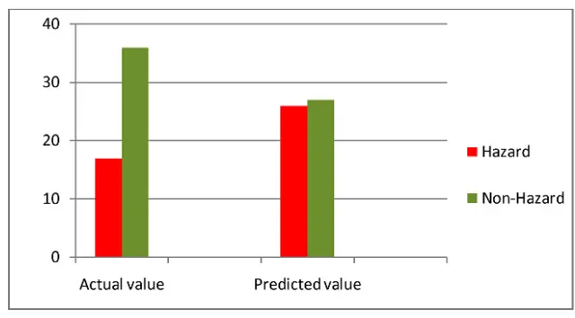
The following histogram (Fig. 4) represents the overall comparison of the actual data and
the predicted values by the model. It was observed that the model predicts few more hazardous situations than the real situation.
Number of
cases buildingModel Validation
Total 250 53
Hazard 125 17 Non-hazard 125 36
Table 3
The following table (Table 4) summarizes the prediction capability of the proposed classification tree model. The measurement of prediction capability was done based on the percentage of error in predicting the actual situation, the higher the error percentage, the less the prediction accuracy.
It is observed that the proposed classification tree has an accuracy of 75.48%. The results of Z test show that this accuracy level is significant. A default model predicting all cases as hazards or non-hazards will gain an
accuracy equal to 50% if dataset contains equal number of hazard and non-hazard cases. To compare the developed model with these hypothetical default models, Z test is conducted. In this test, 50% accuracy is named as P1 and 75.48% accuracy is named as P2. The total samples for P1 and P2 are the number of cases (53 cases) used for validation. The test is one-tailed and the significance level is taken as 0.05. The hypotheses are: Null hypothesis, H0: P1 >= P2 Alternative hypothesis, Ha: P1 < P2
Fig. 4.
Comparative Graph of Predicted and Actual Value of the Accident and Non-Accident Cases
Table 4
Prediction Capability of Classification Tree
Number of cases Wrong prediction % Error
Total 53 13 24.52%
Hazard 17 2 11.76%
In this test, it is found that the value of z is - 2.66. Since this is one tailed test, the P value is the probability that z score is less than -2.66. By using Z Table, it is found that P(z < -2.66) is 0.00334. Since the P value is less than the significance level, the null hypothesis is rejected and alternative hypothesis is accepted. That means the developed model for this study can perform better than the model of 50% accuracy.
8. Discussions
A hazard risk probability model has been developed and its application to evaluate the hazard risks under different traffic conditions on the freeway was demonstrated. Summary and findings of the study are described below:
• In order to predict the crash hazard situations, this study developed a classification tree. This tree was formulated by using traffic parameters i.e. traffic flow and vehicle speed at the upstream and current location during current time, 5 minutes before and 10 minutes before the current time. There are in total 28 criteria included in the tree which shows if there is hazardous or non-hazardous situation. It is found that flow at current location at 5 minutes before current time and flow at current location at 10 minutes before current time have no impact on tree building i.e. hazard situation.
• Although in the initial stages of the model building process, weather conditions such as rainfall intensity was considered as a prediction variable, on further exploration, it has been found that rainfall has no significant impact on hazard occurrence on the freeway.
• It is obser ved that the proposed classification tree has an accuracy of more than 75% which is more significant than any default model consisting of all hazard or all non-hazard cases. Future research can be done in order to improve the accuracy level of the model by including other relevant predictor variables with the existing variables. On the other hand, the accuracy level is much higher (about 88%) in accident cases. On the other hand, this model has more prediction error in non-accident cases which is more than 30%. It may be because the model predicts the hazardous conditions based on the traffic performance indicators while the driver related characteristics for example, alertness and attention which cannot be observed so easily may have avoided the accidents from happening. To improve the accuracy in non-accident cases, fuzzy logic can be implemented in future research. It can be said that the classification model can predict accident cases more correctly than that of non-accident cases.
9. Conclusion
in different traffic control schemes. Future research can be conducted on how to improve the road traffic performance on the freeway in order to reduce hazard risk probabilities by adopting different traffic control strategies.
Acknowledgements
The author is greatly indebted to Dr. Shamas Bajwa for his helpful and expert suggestions. Thanks to Mr. Jude Jusayan and Tim Strickland of Vic Roads and the authority of Bureau of Meteorology (Australia) for providing the data.
References
Aarts, L.; Ingrid, V.S. 2006. Driving speed and the risk of road crashes: A review, Accident Analysis & Prevention, DOI: http://dx.doi.org/10.1016/j.aap.2005.07.004, 38(2): 215-224.
Aljanahi, A.A.M.; Rhodes, A.H.; Metcalfe, A.V. 1999. Speed, speed limits and road traffic accidents under free flow conditions, Accident Analysis & Prevention, DOI: http://dx.doi.org/10.1016/S0001-4575(98)00058-X, 31(1–2): 161-168.
Ayati, E.; Abbasi, E. 2011. Investigation on the role of traffic volume in accidents on urban highways, Journal of Safety Research, DOI: http://dx.doi.org/10.1016/j. jsr.2011.03.006, 42(3): 209-214.
Breiman, L.; Friedman, J.H.; Olshen, R.A.; Stone, C.J. 1984. Classification and regression trees. Wadsworth & Brooks/Cole Advanced Books & Software, Belmont, CA, United States of America.
Dickerson, A.; Peirson, J.; Vickerman, R. 1998. Road accidents and traffic flows: an econometric investigation. Available from Internet: <ftp://ftp.ukc.ac.uk/pub/ejr/ RePEc/ukc/ukcedp/9809.pdf>.
Durduran, S.S. 2010. A decision making system to automatic recognize of traffic accidents on the basis of a GIS platform, Expert Systems with Applications, DOI: http://dx.doi.org/10.1016/j.eswa.2010.04.068, 37(12): 7729-7736.
Eisenberg, D. 2004. The mixed effects of precipitation on traffic crashes, Accident Analysis & Prevention, DOI: http://dx.doi.org/10.1016/S0001-4575(03)00085-X, 36(4): 637-647.
Elvik, R.; Christensen, P.; Amundsen, A. 2004. Speed and road accidents: An evaluation of the Power Model. Institute of Transport Economics, Oslo, Norway. 134 p.
Gang, R.; Zhuping, Z. 2011. Traffic safety forecasting method by particle swarm optimization and support vector machine, Expert Systems with Applications, DOI: http://dx.doi.org/10.1016/j.eswa.2011.02.066, 38(8): 10420-10424.
Golob, T.F.; Recker, W.W.; Alvarez V. 2004. Freeway safety as a function of traffic flow, Accident Analysis & Prevention, DOI: http://dx.doi.org/10.1016/j.aap.2003.09.006, 36(6): 933-946.
Goodwin, L.C. 2002. Weather Impacts on Arterial Traffic Flow. Prepared for the Federal Highway Administration (FHWA) Road Weather Management Program. United States of America. 5 p.
Greibe, P. 2003. Accident prediction models for urban roads, Accident Analysis & Prevention, DOI: http://dx.doi. org/10.1016/S0001-4575(02)00005-2, 35(2): 273-285.
Higgs, R.; Cummins, D. 2003. Recursive Partitioning, Lecture for CHM696D, Statistical & Information Sciences, Lilly Research Laboratories. Available from Internet: <http://miner.chem.purdue.edu/Lectures/Lecture15%20 -%20Higgs_RP.pdf>.
Hong, D.; Kim, J.; Kim, W.; Lee, Y.; Yang, H.C. 2005. Development of traffic accident prediction models by traffic and road characteristics in urban areas. In Proceedings of the Eastern Asia Society for Transportation Studies, Vol. 5: 2046-2061.
Jean-Louis, M. 2002. Relationship between crash rate and hourly traffic flow on interurban motorways, Accident Analysis & Prevention, DOI: http://dx.doi.org/10.1016/ S0001-4575(01)00061-6, 34(5): 619-629.
Kalokota, K.R.; Seneviratne, P.N. 1994. Accident prediction models for two-lane rural highways. Available from Internet: <http://www.mountain-plains.org/pubs/ pdf/MPC94-32.pdf >.
Lord, D.; Manar, A.; Vizioli, A. 2005. Modeling crash-flow-density and crash-flow-V/C ratio relationships for rural and urban freeway segments, Accident Analysis & Prevention, DOI: http://dx.doi.org/10.1016/j.aap.2004.07.003, 37(1): 185-199.
Mustakim, F.; Yusof, I.; Onn, H.; Rahman, I.; Samad, A.A.A.; Salleh, N.E.B.M., 2008. Blackspot Study and Accident Prediction Model Using Multiple Liner Regression. First International Conference on Construction in Developing Countries (ICCIDC–I): Advancing and Integrating Construction Education, Research & Practice. Karachi, Pakistan.
Navon, D. 2003. The paradox of driving speed: two adverse effects on highway accident rate, Accident Analysis & Prevention, DOI: http://dx.doi.org/10.1016/S0001-4575(02)00011-8, 35(3): 361-367.
Ossiander, E.M.; Cummings, P. 2002. Freeway speed limits and traffic fatalities in Washington State, Accident Analysis & Prevention, DOI: http://dx.doi.org/10.1016/ S0001-4575(00)00098-1, 34(1): 13-18.
Pham, M.H.; Bhaskar, A.; Chung, E.; Dumont, A.-G. 2010. Random forest models for identifying motorway Rear-End Crash Risks using disaggregate data. In Proceedings of the 13th International IEEE Conference on Intelligent Transportation Systems (ITSC), DOI: http://dx.doi. org/10.1109/ITSC.2010.5625003. 468-473.
Rujun, Y.; Xiuqing, L. 2010. Study on Traffic Accidents Prediction Model Based on RBF Neural Network. In Proceedings of the 2nd International Conference on Information Engineering and Computer Science (ICIECS), DOI: http://dx.doi.org/10.1109/ICIECS.2010.5678126. 1-4.
Shankar, V.; Fred. M.; Woodrow, B. 1995. Effect of roadway geometrics and environmental factors on rural freeway accident frequencies, Accident Analysis & Prevention, DOI: http://dx.doi.org/10.1016/0001-4575(94)00078-Z, 27(3): 371-389.
Taylor, M.C.; Lynam, D.A.; Baruya, A. 2000. The effects of drivers’ speed on the frequency of road accidents. Road Safety Division, Department of the Environment, Transport and the Regions. United Kingdom. 50 p.
Therneau, T.M.; Atkinson, E.J. 1997. An introduction to recursive partitioning using the RPART routines. Technical report, Mayo Foundation. United States of America. 52 p.
Wang, C.; Quddus, M.A.; Ison, S.G. 2009. Impact of traffic congestion on road accidents: A spatial analysis of the M25 motorway in England, Accident Analysis & Prevention,
ISPITIVANJE UTICAJA SAOBRAĆAJNIH
PARAMETARA NA HAZARDE NA PUTU
PRIMENOM MODELA KLASIFIKACIONOG
STABLA
Md. Mahmud Hasan
Sažetak: U radu je prikazan metod za identifikaciju hazardnih situacija na autoputevima. Za potrebe ove studije, razmatrani su uslovi na sekciji Istočnog autoputa u Melburnu u Australiji na dužini od 18 km. Za analizu i razvoj modela korišćene su tri kategorije podataka: saobraćaj, vremenski uslovi i podaci o udesima. U cilju definisanja modela za procenu rizika od udesa, razvijen je osnovni model zasnovan na klasifikacionom stablu. Pri definisanju modela, utvrđeno je da vremenski uslovi ne utiču na pojavu udesa, pa je klasifikaciono stablo formirano na osnovu dva saobraćajna parametra: protoka saobraćaja i brzine vozila. Pomoću definisanog klasifikacionog stabla, moguće je identifikovati sve potencijalne (ne)hazardne situacije na posmatranom autoputu. Rezultati dobijeni u ovom radu mogu se koristiti za razvoj strategija za smanjenje potencijalnih opasnosti u drumskom saobraćaju na autoputevima.