LAND COVER AND LAND USE CHANGES UNDER FOREST PROTECTION AND RESTORATION IN TIANTANGZHAI TOWNSHIP, ANHUI, CHINA
Qi Zhang
A thesis submitted to the faculty of the University of North Carolina at Chapel Hill in partial fulfillment of the requirements for the degree of Master of Arts in the Department of
Geography.
Chapel Hill 2014
Approved by:
Conghe Song
Xiaodong Chen
ii © 2014 Qi Zhang
iii ABSTRACT
QI ZHANG: Land Cover and Land Use Changes under Forest Protection and Restoration in Tiantangzhai Township, Anhui, China (Under the direction of Conghe Song)
Deforestation and forest regeneration are two key changes in the forest ecosystem that have
profound impacts of the goods and services in terrestrial ecosystem. In late 1990s, China
implemented Sloping Land Conversion Program (SLCP) and Natural Forest Protection
Program (NFPP) aimed at forest protection and restoration. Using archived historical images,
this study compared the land-cover/land-use (LCLU) changes before and after the programs
and developed remote sensing indices to characterize the growth trajectory of
“Grain-For-Green” (GFG) and natural forests. The results indicate substantial increase of natural forest
cover during 2002-2013, compared with that during 1992-2002. The proposed indices
revealed aggradation for both NFPP and GFG forests since the implementation of these
policies. Further analysis found spatial variation of forest development depends on the
topographic factors. This study reveals that SLCP and NFPP have been improving forest
iv
ACKNOWLEDGEMENTS
I take this opportunity to express my profound gratitude and deep regards to my
advisor, Dr. Conghe Song, for his exemplary guidance, monitoring and constant
encouragement throughout the course of this thesis. I offer my sincere appreciation for the
learning opportunities provided by Dr. Lawrence Band and Dr. Xiaodong Chen for their
advices throughout the research.
My completion of this project could not have been accomplished without the support
my research group members: Matthew Dannenberg, Yulong Zhang, Chris Hakkenberg and
Chong Liu. The discussions with them provides me with great thoughts in processing remote
sensing data and interpretation of results. Thanks also to the support of Matthew J. Burbank
summer research fellowship from graduate school of UNC, which provided me the
opportunity for data collection during summer 2013.
I am also deeply grateful to my parents for their help and guidance for my life. Their
valuable and constructive suggestions shall carry me a long way in the journey of life on
v
TABLE OF CONTENTS
LIST OF TABLES ... vii
LIST OF FIGURES ... viii
1. INTRODUCTION ... 1
2. DATA AND METHODS ... 7
2.1 Study area ...7
2.2 Data acquisition and preprocessing ...8
2.3 Classification and change detection ...8
2.3.1 Random forest (RF) classifier ... 8
2.3.2 Automatic Adaptive Signature Generalization (AASG) ... 9
2.3.3 Classification of Landsat images ... 10
2.3.4 Classifying WorldView-2 and “Grain-for-Green” forest stands ... 11
2.4 Landscape Pattern Metrics ...12
2.5 Growth trend of successional forest covers...13
3. RESULTS ... 16
3.1 Land cover and land use change detection ...16
vi
3.3 Spectral/temporal trajectories of all forests ...17
3.3.1 Spatial and temporal pattern of all classes ... 17
3.3.2 Spectral/temporal trajectories with successional indices ... 19
3.4 Growth trend of GFG forest stands based on successional index ...23
3.4.1 Temporal trajectories of GFG forest stands ... 23
3.4.2 Correlations between CI, MI, SynI and vegetation index ... 25
3.4.3 Growth trend of GFG forest stands ... 26
4. DISCUSSION ... 28
4.1 Classifications and landscape analysis ...28
4.2 Temporal trajectories of natural forest ...30
4.3 Growth trend of GFG forest stands ...32
5. CONCLUSIONS ... 33
TABLES ... 35
FIGURES ... 37
vii
LIST OF TABLES
Table
1. Landsat imagery acquired for the year of 1992, 2002 and 2013 ...36
2. Statistics of change detection for forest, shrub/grass land and cropland ...36
3. Interpretation of selected landscape metrics ...36
viii
LIST OF FIGURES
Figure
1. Study area: Tiantangzhai Township at Jinzhai County Anhui, China ... 38
2. Fundamentals of the workflows for the AASG method ... 39
3. Selection of c parameter for given class ... 40
4. The normalized B-G space of Tasseled Cap transformation ... 41
5. Land use and land cover in Tiantangzhai Township ... 42
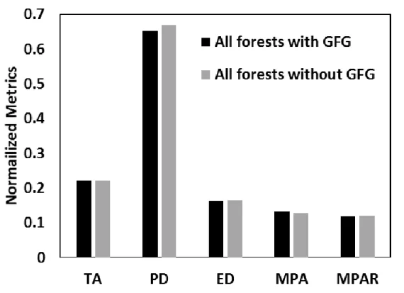
6. Changes of landscape metrics for all forests with and without GFG forest stands at the whole region scale ... 43
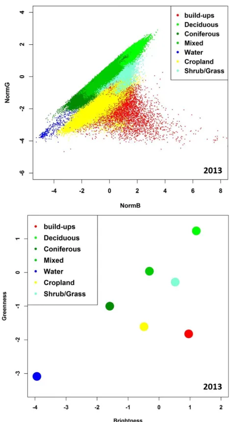
7. Scatter plot (left) and spatial distribution of mean values (right) for build-ups, forests (deciduous, coniferous and mixed forest), water, cropland and shrub/grass of Landsat 8 OLI image (2013) in normalized B-G space ... 44
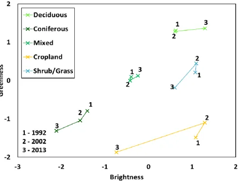
8. Temporal trajectories of stable classes in normalized B-G space ... 45
9. Scatter plot of forest classes with corresponding canopy closure line (CCL) in 2013 ... 45
10.Temporal change of mean distances to the CCL and Li,upper of forest classes (deciduous, coniferous and mixed) and all forests ... 46
11.Temporal change of closure index (CI), maturity index (MI), and synergistic successional index (SynI) of forest classes (deciduous, coniferous and mixed) and all forests ... 47
12.Scatter plot for SynI. The plots above display the temporal change (1992, 2002 and 2013) for all the forests. The plots below are illustration of coniferous, deciduous and mixed in 2013 ... 48
13.Temporal trajectory of all GFG forest stands on average ... 49
14.Temporal change of mean di, Li,upper and CI, MI, SynI for GFG forest stands ... 50
15.Scatter plot for SynI of all the GFG forest stands in 1992, 2002, and 2013 ... 51
ix
17.Topographic indices (elevations, slopes, and aspect) on average
for different levels of GFG forest growing trend based on the change of SynI ... 53
18.Vegetation index (NDVI, NDWI2, EVI, and SI) difference for the three levels of GFG forest based on the change of SynI
between Year 2002 and 2013 ... 54
19.Illustrations of GFG forest stands at levels of a) poor-, b) moderately-
1
1. INTRODUCTION
Land cover and land use (LCLU) change is the main driver of the habitat
fragmentation that resulted changes in essential goods and services provided by the terrestrial
ecosystem (Butchart et al., 2010; Millennium Ecosystem Assessment, 2005; Fischer et al.,
2012; Sieber et al., 2013). LCLU change is sensitive not only to the changes in
environmental conditions but also to human activities. The spatiotemporal dynamics can
significantly modifies the energy exchanges between the Earth’s surface and atmosphere and
therefore the feedback to the society supporting human beings (Otterman 1974; Charney and
Stone 1975; Sagan et al. 1979). It is reported that land cover at global scale has been
transformed under the human use of land resources including agricultural cultivation, pasture
exploitation, forest harvesting, build-up constructions, and the like (Meyer, 1995; Dale et al.,
2000). As the global population rapidly grows, land use activities also alter the landscape
structures by introducing new land cover types which has substantial impacts on the natural
habitats for existing endemic species (Turner et al., 2001). One of the major changes caused
by human activities involving forest cover includes two fundamental types: deforestation and
regeneration (Song et al., 2002; Song et al., 2007). Over decades, forests has been suffering
critical loss particularly in developing countries for agricultural expansions, which posed
high threats to the environment and caused ecosystem degradation (Dobson et al., 1997;
Salim and Ullsten, 1999). Forests are also believed to play crucial role in global carbon
2
forest regrowth may be the major reason for the “missing sink” of carbon budgets (Caspersen
et al., 2000; Myneni et al., 2001; Lelieveld, 2010).
The over-exploitation of forest resources in China caused various problems to the
natural environment in terms of the sustainable development at national scale. After a
half-century forest logging policy, China experienced disastrous droughts in 1997 and floods in
1998, following which the central government implemented a new protection program called
Natural Forest Protection Project (NFPP) in 1998. This new policy was regarded as the
largest logging-ban program in the world, aimed at forest conservation and protection from
forest degradation, biodiversity loss and soil erosion (Zhang et al., 2000; Mullan et al., 2010;
Zheng et al., 2011). Depending on priority levels, the households living in
policy-implemented regions receive different levels of financial support by central government for
managing natural forests without timber harvesting. To expand the existing conservation of
forest ecosystems, China in 2001 has also adopted forest restoration program which
encouraged households to convert their cropland to the forests. These participating lands are
located mainly on steep slopes with low productivity or even abandoned by the farmers.
Therefore, the restoration program is called Sloping Land Conversion Program (SLCP), also
known as “Grain-for-green” program. This program involves a scheme of payment for
ecosystem service (PES) which provides financial support for the participated household
based on the area of converted land to compensate the loss of income from the croplands. A
secondary goal is to alleviate poverty of local farmers (China State Council, 2000; Chen et
al., 2012; Vina et al., 2013; Song et al., 2013). As a result of the forest conservation and
3
harvesting wood and farming work to non-farming labor work except for the compensation
by government support.
The forest programs were evaluated in several provinces of China by researchers and
were believed to be effective for the conversion of marginal cropland to forests as well as
providing financial support to households in poor areas (Wang et al., 2007; Gauvin et al.,
2010; Chen et al., 2010). However, some researchers have reported that China’s preliminary
work on logging bans and forest restoration programs have mixed success with various
limitations which may not be adequate tools for forest management (Durst et al., 2001;
CIFOR REHAB, 2003; WRI, 2003). Many studies also indicated that the performance of the
programs varies strongly depending on different local context (Persha et al., 2011; Song et
al., 2013) and there is limited research particularly on tracking growth trend of the
regenerated forests. There is also concern that the re-conversion from forest or grassland to
cropland and wood harvest of natural forest would be possible if government subsidies were
stopped (Hu et al., 2006; Shen et al., 2006).
Due to the complexity of synergistic effects on the local environment, more extensive
and sophisticated experiments of the forest conservation and rehabilitation programs at local
scale are required for better understanding their influence as well as feedbacks from
ecosystems before scaling up for nationwide policy implementations (Weyerhaeuser et al.,
2005). Advanced tools such as satellite images offer the opportunity to comprehensively
monitor the growth trend of the natural forest and converted forests and thus to offer timely
feedback for the improvement of large programs (Liu et al., 2008). Remote sensing allows
useful approaches in mapping land cover at large scales both spatially and temporally. For
4
one large area while high spatial resolution remotely sensed data such as WorldView-2
images can be used to evaluate the effectiveness of forest cover observation with detail
information. In addition, the combination of remote sensing and GIS serves as a powerful
tool in analyzing the landscape pattern of the earth surface (Serra et al., 2008; Geri et al.,
2010). Landscape ecological concepts and metrics offers fundamental theories for better
understanding of sustainability of land use planning by the applications of landscape
transformation (Leritão and Ahern, 2002; Ribeiro and Lovett, 2009).
In contrast to the conversion of forest to cultivated land, forest regeneration due to
policy implementation pertains much to the study of forest at their early stages with remotely
sensed data (Song and Woodcock, 2002). The land cover changes regarding forest
successional stages can be of significance to the global carbon cycling and conservation of
water resources (Woo et al., 1997; Chen et al., 2002; Preditzer and Euskirchen, 2004). It is
also believed that mapping regenerated forest is much more challenging than mere
deforestation due to the difficulty of monitoring the gradual changes of forest succession
particularly after canopy closure (Pax-Lenney et al., 2001; Song et al., 2007). Several
researchers have devoted efforts to characterize the spectral response of the forests at
different successional stages with remotely sensed imageries. The Tasseled-Cap
Transformation (Kauth and Thomas, 1976), which linearly converts spectral signals of
Landsat Satellite data into meaningful measures of brightness, greenness and wetness, has
proven to be informative in separating young, mature and old-growth forests (Cohen et al.,
1995; Fiorella and Ripple, 1993a). Fiorella and Ripple (1993b) also found a high correlation
between the “structural index” (TM 4/5 ratio) and the age of Douglas-fir stands which can be
5
However, the applications of empirical relationships with single date image by
previous studies are limited due to the high dependence of extraneous factors in terms of
local environmental context (Gemmell, 1999; Gemmell and Varjo, 1999). It is suggested in
several papers that multiple images at various dates should be incorporated to identify the
distribution of forest at different successional stages (Helmer et al., 2000; Lucas et al., 2002).
Song et al (2002) characterized the spectral temporal trajectories for early successional
forests and found several sources of noise such as topography and initial background
conditions could potentially prevent accurate estimate of forest successional stages. The
uncertainties caused by topography, atmospheric condition, phenology and sun/view angles
were further evaluated (Song and Woodcock, 2003; Millan et al., 2013) and the results
indicated that Tasseled Cap indices as well as normalized difference vegetation index
(NDVI) of forests at different stage can be affected by these factors. Song et al. (2007)
simulated the spectral reflectance of forest successions and used regression analysis to fit the
successional trajectories for spectral predictors of Tasseled Cap transformation. The results
showed that the brightness and greenness performed much better than wetness index for
successional forests and also emphasized the monitoring effectiveness of using multitemporal
Landsat imagery based on regression analysis. Overall, more efficient approaches are
required to capture the signatures of subtle changes for successional forest cover while
minimize the noisy effects that contaminate the multitemporal images.
Therefore, two research questions are asked, 1) How does LCLU change before and
after the implementation of SLCP and NFPP around 2000? 2) What is the growth trend of
GFG and natural forests since the implementation of the new policies? The hypotheses
6
natural and GFG forest have positive growth trend of aggradation under the implementation
of forest protection and restoration programs. To investigate these research questions,
Tiantangzhai Township with natural reserve was selected as study area in southeastern Dabie
Mountain of China. The overall objective is to track land cover and land use change before
and after implementation of forest policies as well as to characterize the growth trend of both
natural forest and GFG forest stands since 2002. More specifically, the research was
conducted to: 1) map forest class within Tiantangzhai Township in 1992, 2002, and 2013 and
analyze the forest landscape with/without GFG forest stands; 2) quantify the forest
successional information by utilizing the Tasseled-Cap indices including brightness and
greenness and track the temporal/spectral trajectories of all forest at whole region scale; 3)
provide reference of GFG forest growing trend after SLCP implementation to policy makers
7
2. DATA AND METHODS
2.1 Study area
The Tiantangzhai Township, in Jinzhai County of Anhui province in China, is located
in the eastern part of Dabieshan Mountain (Fig. 1). The township covers an area of 28,914
hectares (ha) with abundant forest biomass. The elevation of the area varies from 300 to 1700
m above sea level. The mild weather and sufficient rainfall, make it an optimal area for
vegetation growth. Due to its remoteness, the region is characterized by low population and
density. The transportation system is poorly-developed and thus brings inconvenience for the
connections to big cities. Though the natural ecosystem is well preserved due to less
intervention of human activities, the normal behavior such as animal hunting, forest
harvesting by local residents still caused problems in environmental protection for decades
before 21st century. On one hand, this region was established as the national reserve for forest
conservation as one part of the entire NFPP in 1998. In response to the program, the
environment was supposed to be protected from human interference, including forest harvest,
wild life hunting. Almost every household owns land covered by natural forest and receives
8.75 RMB/mu each year (1 mu = 1/15 ha) from the central government. The government
implemented SLCP in 2002 in Jinzhai County. Farmers receive an initial compensation of
230 yuan/mu/year for 8 years, and the renewed compensation of 125 yuan/mu/year for
8
small proportion of the entire study area since only one sixth of all the households
participated the forest restoration program.
2.2 Data acquisition and preprocessing
Three Landsat images were acquired in 1992, 2002 and 2013 from “USGS Global
Visualization Viewer” (http://glovis.usgs.gov/). The availability of the imagery was mainly
limited by the cloud coverage. One scene of WorldView-2 image with high spatial resolution
was also requested. Detailed information of the satellite images were shown in Table 1.
Though many algorithms have been proposed for the data without in situ atmospheric
information, Song et al in 2001 suggested that there were limited improvements with more
sophisticated approaches but a simple modified dark object method can have at least equally
good performance for removing atmospheric effects. In order to characterize the spectral
information with vegetation indices such as NDVI, all the Landsat images in this study were
atmospherically corrected using simple dark object subtraction (DOS3) approach and the DN
value was converted to the surface reflectance. The DOS method assumes 1% surface
reflectance caused by the atmospheric conditions and the minimum DN value over one TM
scene can be found at the value with at least 1000 pixels from the peak of the histogram for
each band (Moran et al., 1992; Chavez, 1996). Digital Elevation Model (DEM) with 30 meter
resolution was also obtained and projection including resampling was re-defined in order to
match the Landsat images in terms of the spatial resolution as well as array alignment.
2.3 Classification and change detection
2.3.1 Random forest (RF) classifier
In recent years, many papers argued to use multiple classifiers to generate an
9
sensed images than any with single classifier (Briem et al., 2002; Dietterich, 2002). A new
and powerful statistical classifier proposed by Breiman in 1999 is called Random Forest
(RF), which randomly chooses a set of features among all the included variables (e.g.
spectral bands, topographic indices) to split each node within a single tree (classifier), and
also generates a large number of such trees. The unknown pixel are assigned by voting it to
most popular class from all the tree predictors. Breiman also stated that the generalization
errors for forests always converge to a limit as the number of trees is very large. An
increasing number of researchers employed this classifier in various fields because it
generates high classification accuracy and has the capability of evaluating variable
importance and of modeling complex interactions (Cutler and Stevens, 2006; Archer and
Kimes, 2008). Pal (2005) compare two machine learning classifiers with Landsat Enhanced
Thematic Mapper Plus (ETM+) data and he argued that the random forest classifier has equal
performance in classification accuracy and training time but requires fewer user-defined
parameters. Prasad et al (2006) also tested four statistical algorithms of vegetation mapping
and found the Random Forest was superior in predicting current distribution of tree species.
In this study, random forest classifier was used through all the processes of classification.
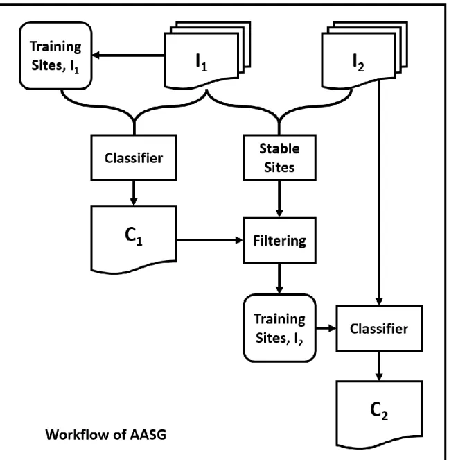
2.3.2 Automatic Adaptive Signature Generalization (AASG)
To keep the consistency of classifications for remotely sensed images with time
series, Automatic Adaptive Signature Generalization (AASG) proposed by Gray and Song
(2013) was employed to adapt spectral signatures of each of the individual Landsat imagery.
This method identifies training data from features that are stable throughout time. It requires
the high accuracy of the most recent image classification to be as the reference image for
10
approach is that the majority of the pixels did not change if the image is for a sufficiently
large area. By subtracting image bands of two different time period, the stable sites within
reliable range can be located around the mode of the histogram of the difference image.
These stable pixels are further filtered and selected as training data to classify their
corresponding image (Fig. 2). Previous study indicated that the AASG is flexible with
respect to any supervised classification algorithm and showed a better performance for
irregular time series comparing with traditional signature extension.
2.3.3 Classification of Landsat images
In this research, random forest (RF) was selected as the classifier for both the
reference map and the AASG approach. Considering the prevalence of vegetation over the
mountainous area of this study site, spectral and topographic derivatives were generated from
remote sensing images as well as ancillary data in order to increase the separability of the
classes. A set of vegetation indices were calculated from the atmospherically corrected
images including simple ratio (Jordan, 1969), normalized difference vegetation index (Rouse
et al., 1973), structural index (Fiorella and Ripple, 1993a), modified normalized difference
water index (McFeeters, 1996; Xu, 2006), enhanced vegetation index (Huete et al., 1997).
Several topographic indices were also derived from digital elevation model (DEM) dataset
including: elevation, slope, aspect, topographic wetness index (Beven and Kirkby, 1979).
To create the reference map of 2013/5/21 Landsat image, the RF classifier was
trained with user defined pixels by referring to the high spatial resolution image
WorldView-2 (WorldView-2013/7/13). The training sites for the WVWorldView-2 image were collected in the field with the
assistance of GPS during summer 2013. Twenty percentage of the pixel values as training
11
for the reference map. Based on the experience and local knowledge of the land use within
study sites, nine land cover types were defined: build-ups, deciduous forest, coniferous forest
mixed forest, water, cropland, rock outcrop, and barren area, and shrub/grass.
In generating the classified maps for target images (Landsat image of 1992/10/18 and
2002/10/6), the AASG method was modified and improved based on Gray and Song (2013).
Firstly, the NDVI band calculated from red band and near infrared band was chosen for
image differencing instead of merely using red band or near infrared band. Because the study
area was dominated by vegetation, including both the near infrared band and the red band
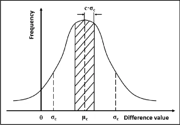
therefore contains more information associated with the stable sites. Second, multiple c
parameter for each class was defined instead of using global c parameter which defines the
thresholds of selecting stable sites. In Gray and Song (2013), the global c parameter of 1, 0.5
and 0.25 were selected to test the threshold sensitivity which may cause the overabundance
problem of stable sites for a particular class such as vegetation. So the c parameter was set by
restricting the number of stable pixels to 1000 with each class in this study. If the total
number of stable pixels is less than 1000, then the interval would be limited to match the
number all pixels for such stable sites of the class (Fig. 3). Third, since AASG is flexible for
any classifier, the random forest was again used in this approach and also was trained by the
extraction of the spectral information, vegetation indices and topographic properties of those
pixels selected as training sites.
2.3.4 Classifying WorldView-2 image and “Grain-for-Green” forest stands delineation
Due to the high spatial resolution of the WorldView-2 image, the classified map as
foreseen can be filled with “speckle” noise particularly for those with high spectral variations
12
some classes such as build-up areas, agricultural land. The specific categories within one
general group were then combined as one class. The general classes were: build-up area
(open, pitch, residents), water (river, pond), forest (deciduous, coniferous, mixed), farmland
(cropland, dry land), barren land (rock, open). The clouds associated with their shadows were
removed from the entire scene. A 5 by 5moving window majority filtering was carried out to
reduce the speckles.
It is challenging to identify the “Grain-for-Green” (GFG) forests merely based on the
satellite image itself because of the confusion with natural forests in terms of the spectral
information. Additional data were acquired including topographic map depicting each GFG
forest stands associated with the ID, location and area, and the data that monitored the
progress of GFG forest by households in 2009. The technician in the local township forest
station also provided personal experience on locate each GFG patch on the WorldView-2
image. 226 GFG forest stands were depicted in ArcGIS and exported as a vector layer of
GFG forest class. Fortunately, all the forest stands are free of the cloud cover. The vector
layer were then stacked to the Landsat images for further analysis of forest growth trend.
2.4 Landscape Pattern Metrics
During the past decades, numerous landscape pattern metrics have been proposed for
analyzing the composition and configuration of landscape structure and spatial patterns as
well as their application in relationship with the sustainability for land planning (Turner and
Gardner, 1991; Ribeiro and Lovett, 2009; Su et al., 2011). The changes in landscape structure
triggered by the land use/cover change has strong influences on the changes of ecosystem
functions and vice versa (Leitão and Ahern, 2002). The landscape process measurements of
13
the change of biodiversity. In this study, a set of class-level metrics based on the research
questions were selected including total area (TA), patch density (PD), edge density (ED),
mean patch area (MPA), mean perimeter area ration (MPAR). The calculated metrics were
then used to compare the landscape patterns between natural forest without GFG forest
stands and all the forest including GFG forests. It was also applied to the each forest class
including deciduous, coniferous and mixed forest.
2.5 Growth trend of successional forest covers
The growth trend of the GFG forests stands pertains to the monitoring of forest
successional change which has implications for land use management as a fundamental
ecological process (Song et al., 2002). In this research, the temporal trajectories of the GFG
forests were examined in the brightness and green space (B-G space). The pixels of forests
were generally spread along a line in the B-G space, which is regarded as canopy closure line
(CCL) in this study. Once the canopy were closed, the forests at early stages located at the
higher end of CCL with both high brightness and greenness values. As forest succession
continues, increased mutual shadowing in the canopy leads to the decrease of both brightness
and greenness. As a result, forests move towards the lower end of CCL as they mature. In
order for the multitemporal image data to be comparable, both brightness and greenness were
normalized to Z-score values separately.
The CCL was defined as a parallel segment of the linear regression line of points at
left side of the tasseled cap. Given small ranges of greenness, the points with the lowest
brightness within each range were filtered as candidate points on the canopy closure line. A
14
lower bound of the segment are limited by the maximum and minimum vertical points of the
pixels respectively (Fig. 4).
The successional information of forests was considered as a combination of two
indices: closure index (CI) and maturity index (MI). The closure index is related to the
perpendicular distance of a given point to the canopy closure line and is estimated as:
𝐶𝐼 =(𝑑𝑚𝑎𝑥− 𝑑𝑖)
𝑑𝑚𝑎𝑥 (1)
Where dmax is the distance of the pixel which has the largest distance to the CCL, di is
the distance of the ith pixel to the CCL. The larger the value is, the more the pixel is likely to
be forest with closed canopy. The other index represent which group of successional stage
the forest belong to and is estimated as:
𝑀𝐼 = 𝐿𝑖,𝑢𝑝𝑝𝑒𝑟
𝐿 (2)
Where Li,upper is the length of segment at CCL between vertical point of a given pixel
and the upper bound along CCL, and L is the length of CCL between upper bound and lower
bound. The CI and MI each have limitation to represent the successional information, so a
synergistic successional index called SynI was developed as the product of these two indices:
𝑆𝑦𝑛𝐼 =(𝑑𝑚𝑎𝑥 − 𝑑𝑖)
𝑑𝑚𝑎𝑥 ×
𝐿𝑖,𝑢𝑝𝑝𝑒𝑟
𝐿 (3)
The index values of CI, MI, and SynI all ranges from 0 to 1. The SynI represents a
combined information of both canopy closure and successions. The larger value denotes that
the forest pixel is closer to old-growth forests and lower to the young forests.
Regressions with vegetation indices proposed by previous studies was conducted for
each year to evaluate the actual meanings of these indices generated. Then the GFG forest
15
order to monitor the growing trend of these planted trees. The topographic and vegetation
16 3. RESULTS
3.1 Land cover and land use change detection
The classified maps of the three Landsat images are shown in Fig. 5. The 2013
classification as reference image has overall 92% accuracy with Kappa coefficient over 0.9.
The classifications in Year 1992 and 2002 were generated using AASG methods. The change
detection statistics for forest, cropland and shrub/grass land were summarized in Table 2.
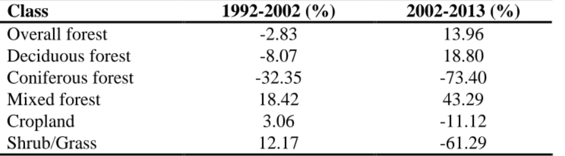
From 1992 to 2002, the overall forest area does not change much while there is 13.96%
increase from 2002 to 2013. Before the implementation of forest conservation and restoration
programs, the areas of deciduous and coniferous forests declined while that of mixed forests
increased. However, during the decade after the program, deciduous and mixed forests both
have substantial increases in study area. The tree species provided by the government for the
program were mainly deciduous forests which have relatively higher survival rates.
The cropland had limited increase before the SLCP implementation and declined by
11.12% partially because of the conversion from participated farmland to the GFG forests. It
is also notable that there is great amount of decrease for shrub/grass land (-61.29%). The
shrub and grass land have the largest confusions over all the classification particularly at the
boundary between forest cover and non-forest vegetation land cover. The major
transformation has occurred from the shrub/grass land to the deciduous and mixed forests.
The natural forests and the young trees planted by local residents have gradually become the
17 3.2 Synoptic forest landscape pattern change
The class-level analysis of landscape metrics offers a general landscape pattern of
forest including GFG stands and excluding GFG stands (Fig. 6). The interpretations for each
metric were summarized in Table 3. Since the total area of GFG forest stands is relatively
small compared with the natural forests within the township, the landscape characteristics
generally have little changes for the forest covers with and without GFG forests. Though the
decrease of total area for forest without GFG forest is negligible, such slight changes can be
observed via other metrics that all the forest cover with GFG forests were less fragmented at
class level with 2.6% higher of patch density and 1.1% higher of edge density if the GFG
forest were clipped out. The lower, not substantial though, mean patch area (MPA) and mean
ratio of perimeter to area (MPAR) of forests indicated the irregularity and complexity of the
forest patches without GFG forests.
3.3 Spectral/temporal trajectories of all forests
3.3.1 Spatial and temporal pattern of all classes
The scatter plot of transformed “tasseled cap” of Landsat 8 OLI image of 2013 is
shown in Fig. 7. It should be noted that the data points are so dense that the majority of them
were overlapped, particularly for deciduous, coniferous and mixed forests. So the mean
values of normalized brightness and greenness of each class are also plotted to clearly display
the spectral distribution in brightness-greenness (B-G) space of Tasseled Cap transformation.
The classes of barren land and open rock, accounting for a tiny portion of the entire study
area, were excluded in the figures. The relative patterns of each class indicates that forests
are compactly spread along a line on the upper left side of the “tasseled cap” with higher
18
measured surface reflectance is mainly from the vegetation with limited contribution from
the background. Along this canopy closure line, it is believed that both greenness and
brightness decrease as the forest grows because of mutual shading as the trees getting bigger.
The deciduous forest, colored in light green in Fig. 7 has higher values of both brightness and
greenness due to higher reflectance from broad leaf species. The coniferous forest, colored in
dark green in Fig. 7, appears to have lower values in both brightness and greenness due to its
relatively lower reflectance compared with the broad leaf species. Mixed forest accounting
for the majority of forest pixels is located between deciduous and coniferous forest with
wider spread due to its higher variety in terms of spectral signature. The shrub/grass land also
have relative higher brightness and greenness but below the forest at canopy closure line.
This is reasonable due to the sunlit background in addition to their high reflectance at green
wavelength. The cropland, however, is located below the forest and shrub/grass cover with
points widely spread due to the properties of various crops planted. There is variety of crops
during the time of image acquisition, ranging from the higher brightness for open land after
the crop harvest, and other crops at varying stage of development. The water class has the
lowest surface reflectance, and thus is neither bright nor green. The complexity of the
build-up class make it possible that the points widely spread in the B-G space but generally have
high brightness and low greenness due to the spectral properties associated with concrete,
pitch, cement in the residential areas. Similar spectral patterns of Tasseled Cap
transformation were also observed for Landsat 5 TM image in 1992 and Landsat 7 ETM+
image in 2002.
The stable pixels of forest, cropland and shrub/grass class in all three years were
19
the dominating class in the study area, is the most stable class of spectral signature through
the two decades. The temporal trajectories of mixed/deciduous forests are different from that
of coniferous forest. During the two decades, mixed and deciduous forests are basically
stable with little changes for both brightness and greenness. While coniferous forest keeps
moving to the old-growth during the two decades. This can be attributed to the occupation of
young pioneer trees at early stage on the shrub/grass land triggered by the implementation of
forest conservation and restoration programs. The amount of the conversion from shrub/grass
to deciduous forest is relatively large and it thus leads to the movement of such forest
spectral signals towards early successional stages with increase of both brightness and
greenness. The large change of the cropland between 1992 and 2013 may due to multiple
reasons such as the activities of cultivation by local farmers as well as phenological
responses of crops to the seasonal weather changes. Despite the temporal change of stable
classes, the general spatial pattern maintains that there are no overlap among temporal
trajectories of any two classes in terms of the mean values.
3.3.2 Spectral/temporal trajectories with successional indices
Fig. 9 provides an illustration of depicting canopy closure line (CCL) in B-G space of
2013 Landsat 8 OLI image. Assuming a reasonable accuracy of classification, the pixels of
forest are located closer to CCL than those of other classes. So only points classified as
forests were plotted to define the canopy closure line, which is assumed to be above all the
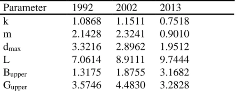
points of the study area. In the case of 2013 image, the greenness value of the pixel with
minimum brightness is 2.6215 and the maximum greenness value is 2.9024. Small steps of
0.01 for greenness from 2.63 to 2.91 was set to identify all the points required on defining
20
the points from all steps were identified, we can fit a regression line as the CCL. Keeping the
slope (0.7518) fixed, the trend line was shifted until all the points were at or below it, which
leads to an intercept of 0.9010 for the 2013 Landsat 8 OLI image. The line was then
segmented with regard to upper and lower bound based on the pixels. The parameters for
defining successional indices for all the three years were listed in Table 4. The upper bound
of brightness and greenness and length of the CCL were used for calculating maturity index.
The temporal changes of mean distance to CCL and the Li,upper of CCL for all forests
and each forest category were examined in Fig. 10. It is not surprising that there is
consistency between these two quantitative measures and the visual observation in temporal
trajectory of each class. From 1992 to 2002, the mean value of distance to CCL for all
categories has modest increase and a significant decline during the next decade, indicating
increase of canopy closure since 2002. As for the Li,upper of CCL for a given pixel in the B-G
space, the mean values for all categories except coniferous forest have increased during the
first decade and moderately declined during the following decade. For similar reasons, this
may also be attributed to the conversion from non-forest vegetation to the young forests,
most of which belong to the deciduous forest or contribute to the mixed forest.
Different from the distance to the CCL and the Li,upper of CCL, the SynI index was
developed as a relative measure over all the forest pixels given one point within the study
area. Therefore the temporal change of the di and Li,upper can be different from this index that
the latter more accurate in measuring the successional stage of a pixel relative over the entire
forested pixels (Fig. 11). It can be observed that the closure index has decreased from 1992 to
2002 and increased rapidly since the forest programs, which indicates the changes in terms of
21
patterns of mean closure index are similar for all the four categories. For maturity index,
however, the temporal trends are different, particularly for coniferous forest. Though the
overall values decreased from 2002 to 2013, the relatively higher magnitude of CCL length
increase over that of distance to CCL upper bound leads to slight decline of maturity index.
Vertically, coniferous forest has highest value and deciduous has the lowest, which agrees
with the results that deciduous forests are at early successional stage while coniferous forest
is mainly at old-growth stage. The product of these two indices (SynI) were calculated to the
track the temporal change of the forest at different successional stages. Seen from Fig. 11, the
SynI values follow the patterns of maturity index across forest classes because of the higher
magnitude of maturity index. However, the temporal changes are slightly different from CI
and MI. In general, the deciduous forest at bottom did not change significantly during the
two decades while the index values for coniferous and mixed forests have increased after the
implementation of programs. The aggradation of coniferous and mixed forests may result
from the conservation of the natural forests that trees in remote area were protected from
logging by local residents. The stable change of deciduous forest may due to both the
restoration of GFG forest stands and conversions from other land covers. The plant of trees
contributed to the increase of closure index while the transformation of land covers caused
the decline of maturity index.
The scatter plot shows the successional synergistic index of all the forest pixels in
1992, 2002 and 2013 (Fig. 12). The overall distributions of index levels are similar that
higher values of SynI are located at the lower left corner in the brightness and greenness
space. As the brightness and greenness increase, the SynI value decreases to 0 closer to the
22
are spread more widely than those in 2013 when the pixels are packed more closely towrds
the CCL. This is because there are more pixels having lower SynI values resulting from the
lower values of MI for the first two years. The changes of observed spectral trajectories in
1992 and 2002 in terms of the spread of high SynI values. In 2013, the highest value
representing the old-growth forest is close to 1 with the indication of late succssions of these
forest pixels which were actully classified as coniferous forest. This distinct phenomenon in
2013 is probably a result from the forest protection and restoration programs. The majority of
the pixels in forest area with initial low SynI tend to move faster to the CCL in response to
the natural growth in mountainous environment. Actually, there are larger amount of pixels
with higher CI values (not shown in the figure) in 2013 indicating the increase of number of
stand with closed canopy, thought the MI values don not change much. Besides, the
proportion of very low CI values for all forest in 2013 is smaller than those in 2002 also
confirms forest aggradation in the recent decade.
The scatter plots of SynI for deciduous, coniferous and mixed forests in 2013 were
displayed in Fig. 12. It is observable that the deciduous forest dominate those at early
successional stage with very low SynI values while coniferous forest has more pixels with
high values than the other two categories except for a small group of pixels. This is probably
because of the misclassification in land cover mapping due to topographic shadow effects.
Within the mountainous region, the deciduous forest at the shading aspect have much lower
reflectance of solar radiation and may appear dark green resembling that of coniferous forest.
After Tasseled Cap transformation and normalization of brightness/greenness, this group of
23
3.4 Growth trend of GFG forest stands based on successional index
3.4.1 Temporal trajectories of GFG forest stands
Based on the topographic map with GFG forest locations marked as a polygon, GFG
stands were manually delineated on the WorldView-2 image. There are a total of 226 GFG
stands in total for the Tiantangzhai Township. The polygons was then overlaid on Landsat
images to extract the brightness and greenness values for these polygons. All the stands
approved by local forest station are included regardless of the actual ground conditions.
Therefore, a group of pixels labeling as GFG forest stands may be classified as non-forest in
the Landsat classification and thus may not be properly measured by the forest successional
indices developed earlier in this study. The temporal trajectory of the average GFG forest in
normalized B-G space was shown in Fig. 13. From 1992 to 2002, the overall brightness of
land to be GFG forest is stable with little change while the increase of greenness is observed.
This if primarily caused by the conversion of planted crops to grass cover. Before 2002, these
GFG forest stands should be recognized as croplands. The participated patches of lands were
considered by local farmers as to be poorly productive. The trajectory, after 2002, has
changed its direction towards less bright and green as GFG forest established. This can be
explained as the result of successional forest creating shadows within the forest stands.
The termporal changes of distance to CCL and Li,upper as well as the forest
development indices were plotted in Fig. 14. The SynI values for GFG forest stands are less
than 0.2 in 1992 and 2002 but increase to 0.24 in 2013. Meanwhile, the extent to which the
CI increase (greater than 0.5) also has taken place in the recent 10 years. During the first
decade, there was not much change because these indices were meaningful for pixels defined
24
decade before and after the implementation of forest programs. As stands were established in
2002, the conversion from croplands to froests have stronger influence to CI derived from the
distance to CCL. Such critical change is reasonable because of the replacement of tree
canopy over the backgound. The MI does not change during the two decades though there is
slight increase of Li,upper from 2002 to 2013. This follows that the planted trees caused the
movement of pixels to lower brightness and greenness along CCL, but contibuted to more
young forest relative to the natural forests around. The incease of the SynI after forest
restoration program demonstrates the overall aggradation of the GFG stands which is mainly
from the large magnitude of increase in CI.
Fig. 15 shows the scatter plots for each group of pixels labeled as GFG forest stands
through the two decades. The pixels with negative mean values were filtered out, meaning
the distance on average to the CCL was even larger than the maximum for natural forests.
These forest stands were regarded as trees that have not met the criteria of well growth until
2013. In this part, 15, 20 and 3 GFG forest stands were excluded from the scatter plot of
1992, 2002 and 2013 respectivly. On one hand, the points for 1992 and 2002 spread wider in
the normalized B-G space and the majority of them have low values (less than 0.5) in terms
of the succession SynI; on the other hand, those GFG forest stands in 2013 are more compact
and the highest SynI value is over 0.54 colored in light green at lower left of the B-G space.
It can be found that the distribution as well as the SynI value are able to characterize the
change for the GFG stands since the implementation of forest plocies, particularly the
restoration program. The overall tendancy of the pixels within GFG forest stand is closer
towards the CCL in 2013. Furthermore, the highest SynI values with both low brightness and
25
3.4.2 Correlations between CI, MI, SynI and vegetation index
To examine the implications of the developed forest indices, regression analysis was
employed to find the correlations between these indices for GFG forest stands and vegetation
indices in previous studies. The illustration of the regression results of forest successional
indices and strucutral index (SI, badn ratio of TM 4/5) in 2013 were shown in Fig. 16 (other
correlations not shown).Among all the possible vegetation indices, the structural index (TM
4/5 ratio) proposed by Fiorella and Ripple (1993) were found to be positively correlated to CI
and SynI for all the three years (R2>0.7), but the relationship is weak for maturity
index(R2=0.16). Such high correlation is believed to result from the strong relationship
between forest canopy and structural characteristics. As stand age class falling into 0-10, the
growing leaves can be determining factors that influence the characteristics of canopy
structure which at the same time promote the canopy closure. Previous studies (Running et
al., 1989) also mentioned that the structural index can not distinguished old-growth forest
with young forest before the canopy closure which explains the poor connection of MI and SI
values. For 2013, interestingly, saturation problem of structural index occurs as the SynI
increases in the regression with relatively low R2 (0.31) comparing with that for CI. This
numerically is because of inverse change ,limited though, of SI with change of MI. Also
notice that the variation SI is getting larger as MI increase. This provides the evidence of
insensitivity of structural index to the extent of forest maturity with age regarding the
successional stages. After the saturated point in SynI-SI regression of 2013, the SynI has
better capapbility of tacking the successional information on both maturity and canopy
closure that SI yet reaches the highest values and keeps unchangeable. In fact, MI values are
26
EVI was developed by adding spectral information from blue band to red and near infrared
bands of Landsat image in order to minimize the effects of background and atmophere (Jiang
et al., 2008). This vegetation index is senitive in monitoring tree growth particularly with
abundant biomass and hence less prone to be saturated which also is applied to the MI
proposed in this study. As for the normalized difference vegetation index (NDVI), the
correlations with CI or MI are roughly around 0.5 but much weaker for SynI with strong
saturation problem of NDVI values.
3.4.3 Growth trend of GFG forest stands
Regarding the potential of forest indices for measuring forest successional
information, the difference of SynI between 2002 and 2013 was taken as an indicator for
estimating the growth trend of GFG forest stands. Among all the forest stands, 3 levels of the
extent to which the trees have been growing were developed: poor-developed, moderately
developed and well-developed. Considering the mountainous area of this natural reserve, the
topographic effects should be taken into consideration for examination. The topographic
information and vegetation indices were then extracted for each level to evaluate the effects
on the growing trees at early stages. Fig. 17 a), b) and c) show the distributions of elevation,
slope and aspect of GFG forest stands with different levels. The well-developed GFG forests
are mainly located in area with lower elevation and flatter slopes, with which the natural
environment may be suitable for the natural growth of trees planted. Furthermore, it is more
likely that such topographic conditions allow easier access for household to manage the
forests particularly during the first few years. For the well-developed forest stands, the
largest proportion lies around aspect facing southwest while that for poor-developed were
27
direction. The temperature over the whole study area has little fluctuation through decades
plus sufficient precipitation, the sunlight therefore can be the primary limitation for GFG
forest growth. The southwestern solar radiation received by trees provides with abundant
energy for photosynthesis meanwhile minimized the shadow fraction caused by canopy of
surrounding forests. Moreover, the fraction of shadowed canopy by GFG forest themselves
can also lead to the change of brightness/greenness and thus the forest indices developed.
Fig. 18 shows the vegetation index changes of the 3 development levels of GFG
forest based on the SynI difference. The plots consolidates the growth trend of aggradation
for the trees planted since 2002. All the vegetation index values are positive with indication
of the general aggradation of GFG forests. Larger differences of the calculated vegetation
indices are observed for well-developed forest stands comparing with
moderately-/poor-developed stands. As a result, the growth trend of the 3 levels can be well-detected using the
measurement of successional forest index in terms of the evaluation by the vegetation
28
4. DISCUSSION
4.1 Classifications and landscape analysis
This study tracked the land use land cover changes in Tiantangzhai Township under
the implementation of forest policies at the beginning of 21st century. The classification for
change detection and landscape pattern characterization emphasized the natural forest and
GFG forest stands in response to natural forest protection and Grain-for-green forest
restoration respectively. In this case, the machine learning method called random forest (RF)
as the classifier was employed and modified automatic adaptive signature generalization
(AASG) as the approach extracting image-based training sites was used for all the process
with remotely sensed data. As pointed out by Gray and Song in 2013, the error sources of
AASG were mainly from the misclassification of reference image and the filtering of stable
pixels with multitemporal imageries. The high quality of classifying the reference map (2013
Landsat OLI image) was satisfied by referring to the fine spatial resolution image from
WV-2 satellite as well as the GPS points collected in field work during summer WV-2013. The overall
accuracy over 90% of the initial reference map ensured the minimization of the accumulated
errors for further classifications. The modifications of AASG approach include adding bands
of vegetation indices and Tasseled Cap indices, which make it necessary for absolute
atmospheric correction in converting DN values to reflectance scaled from 0 to 1. Because
Landsat OLI product was released in 16-bit radiometric resolution, ridge method was also
29
of the most recent one in response to the sensor difference. This also leads to the process of
normalizing brightness and greenness indices separately after Tasseled Cap transformation.
Although the 2013 reference map was generated with high accuracy especially for the
natural forest, there may still exist substantial amount of misclassified pixels for each specific
forest category when applying automatic stable sites due to multiple factors. The change
detection statistics revealed a large difference of conversion among deciduous, coniferous
and mixed forest, on which the phenological change may have strong effects. The dates
acquiring 2013 OLI remotely sensed data is May 21 in early summer but the previous images
(1992 and 2002) were captured by satellites during October. The seasonal change of
vegetation, though not as critical as cropland, accounts for a certain amount of the land cover
change areas over natural forests and shrub/grass land classified. The sun angels across the
seasons should also be taken into consideration. The sun light with higher elevation angle in
during May could have more penetration to the forest canopy which further causes less
reflected signals received by the sensor. Besides, the topographic effects is another error
sources influencing the brightness reflected by trees at sloping facing different directions.
One of the limitations of AASG approach lies in the selection of stable pixels based on band
subtraction that contains nothing but reflectance information. Future improvements may
consider the inclusion of topographic effects for training samples filtering in addition to the
classifier.
The landscape pattern change with conversions of pieces of land to GFG forest is not
significant mainly because of three reasons. Firstly, almost every household own the natural
forest protected from logging but only about a sixth of them participated in Grain-For-Green
30
much less contribution to substantial change of class-level metrics at the entire landscape of
study region. Though the general pattern indicate less fragmentation of forest as GFG forest
established, the metric analysis at patch-level may be more sensitive to young growing trees
over the large scale. Second, the GFG forest identification was referenced on the data from
topographic map decade ago. The accuracy of location and area for each GFG forest stand
basically depends on the personal experiences by local farmer and staff from forest stations.
Since the establishment of trees, it is further hard to monitor the growing trend of each forest
stand particularly for those at remote region with limited access. Thirdly, the forest at early
successional stage can leads to confusions with natural forest and other class such as
abundant shrub/grass due to their weak contribution in terms of reflectance observed from
satellite images. As a result, it is inevitable that some stands labeled as GFG forest have
actually been poorly-developed and thus classified as non-forest cover. These factors overall
undermined the positive impacts of the planted young trees to the natural forest as a whole.
4.2 Temporal trajectories of natural forest
Considering the limitations of classification in forests at different successional stages,
this study proposed the development of forest indices extracting mature and canopy closure
information from the brightness/greenness space after Tasseled Cap transformation. It is
required to generate high quality classification maps because the distribution of the each
class is crucial for calculating the forest indices. This was examined by the spatial/temporal
characterizations of pixels with each class in the normalized brightness/greenness space. The
assumption lies in the relative positions of each category particularly forests when defining
the upper/lower bounds along the canopy closure line as well as the maximum distance to the
31
absolute value of the length of CCL and distance to CCL are in fact incomparable among
multitemporal data. Multiple factors can result in this discrepancy in forming Tasseled Cap.
One of the reasons includes the environmental stress on the forests over the entire
Tiantangzhai Township. According to the sensitivity of vegetation area to the precipitation,
for example, the overall greenness may shifted down in response to drier conditions. Besides,
sensor difference also occur even the coded DN value was converted back to the surface
reflectance and such transforming process of reflecting signals would inevitably cause
information loss and thus influence the distributions of pixels in B-G space.
Therefore the relative location of given pixel over all the points spreading in B-G
space was considered within tasseled cap which also normalizes the value to the range of 0-1.
In this research, CI and MI are relevant to the maximum distance to CCL and length of CCL
respectively with restriction to the pixels classified as forest cover. It is possible to generalize
the restriction to the points within the whole study area. For example, noticing the
distribution of build-up with much higher brightness and lower greenness than other class, its
mean value of B-G coordinates can be a candidate for determining the maximum distance to
CCL. As for the MI based on CCL length, forest pixels seems to be adequate in defining the
upper and lower bound.
Due to the fact that the forest indices are derived from the tasseled cap indices of
forest cover, the actual meaning is confined to the quatification of forest successional
information. Though band math is plausible for creating the index bands, the pixels over the
defined “maximum” distance to CCL would have negative values meaning nothing further
from unlikely forest. This also happened when the pixel lies outside the CCL bounds. Seen
32
classified as build-ups, cropland and water would have negative index values. At this point,
the sensitivity of the defining maximum distance and bounds along CCL was suggested for
further analysis. The selection of study area should also be taken into account with certain
size dominated by forest.
4.3 Growth trend of GFG forest stands
A certain amount of pixels labeled within GFG forest stands have negative value of SynI for
all the three years. It is reasonable for the images in 1992 and 2002 since those patches
depicted were actually cropland or abandoned land belonging to non-forest cover. However,
negative values also exist for the image in 2013. Except for the errors from
misinterpretations, it is likely that the ground truth of these pixels within GFG forest stands
are non-forest due to the growing failure of trees since established in 2002. These pixel with
negative value, as a result, are regarded as the non-forest and removed from the scatter plot
with z-valued ranged 0-1. However, all the pixels were included for calculating the mean
indices to measure the extent of stand aggradation or degradation. The purpose is to track the
growth trend of each forest stand during the decade of forest policy implementation which
manifests the advantages of remotely sensed data in monitoring forest at early successional
stage over the in situ management. Fig. 19 provides the illustrations of forest stands at
different levels on WorldView-2 image in 2013. It can be observed that the well-developed
forest (a) stand has more homogeneous canopy cover while the area of grass/shrub
background is outstanding within the poorly-developed stand (c). It is more likely to cause
negative SynI value when there is large open area of background with higher brightness. For
the moderately-developed stand (b), the canopy closure status undermine the CI value despite
33
5. CONCLUSIONS
Since 2002, substantial land cover changes have taken place following the
implementations of forest conservation and restoration programs in Tiantangzhai Township
until 2013 compared with the changes during the decade from 1992 to 2002. Overall natural
forests prevail the study area with an increase of 14 percent. Large amount of shrub/grass
lands have been converted to other land covers. The decline of cropland was also observed
after the Grain-For-Green program. Though subtle, landscape metric analysis revealed that
the forest landscape became the less fragmented and isolated for all the forest as well as each
forest category (deciduous, coniferous and mixed) when the GFG forest stands were
included. Such subtle changes require accurate spectral signals to characterize change
associated with forest succession.
The development of forest succession were examined in the brightness/greenness
space of the Tasseled Cap transformation. The distribution of pixels classified as forest in the
brightness/greenness (B-G) space makes it possible to characterize the forest at different
successional stages. In this study, 3 indices for forest development were developed in the
brightness/greenness space. The closure index (CI) is relevant to the distance of given pixel
to the canopy closure line which is defined as the regression line along the left edge of the
tasseled cap. This index can be used as an indicator of the canopy structure as it has strong
34
the stand is growing. Along the CCL, the pixels of young forest mainly lie at the top of
tasseled cap with higher brightness and greenness. As the forest develops, the brightness and
greenness value decrease. The synergistic successional index (SynI) was calculated as the
product of CI and MI in order to combine the information from both. Regressions of the
forest indices with vegetation indices indicates that SynI is highly correlated with SI, but
more sensitive to young forests that has not reached canopy closure. In 2013, the pixels of all
forests are packed more closely to the CCL in normalized B-G space indicating forests are
generally in aggradation which can also be characterized by the increase of SynI values.
The temporal trajectory of GFG forest stands showed the spectral signals of changing
brightness and greenness through 20 years. From 1992 to 2002, there is substantial increase
of greenness with stable brightness which is due to the establishment of tress on pieces of
land. During the following decade, both brightness and greenness declined as the young
forests grew. The planted young trees impacted the change of CI, leading to the increase of
SynI. The overall aggradation for GFG forest stands was also observed. Based on the extent
to which SynI increase, the GFG forest stands were divided in to 3 levels poorly-developed,
moderately-developed and well-developed. The topographic effects were observed within
different levels that the stands with positive growing trend are more likely to appear at lower
elevation and gentler slopes facing southeast with sufficient solar radiation. The growth trend
with different level was also examined by the measures of vegetation indices. For validation
of these indices proposed, in situ data were required measuring the actual reflectance of each
forest category and testing the sensitivity of the defining the distance to CCL as well as
35 TABLES
Table 1. Landsat imagery acquired for the year of 1992, 2002 and 2013 (Path/Row: 122/38)
Year Date Satellite Sensor Multispectral resolution
Panchromatic resolution
1992 October 18 Landsat 5 TM 30 m 15 m
2002 October 6 Landsat 7 ETM+ 30 m 15 m
2013 May 21 Landsat 8 OLI 30 m 15 m
2013 July 13 WorldView-2 - 2 m 0.5 m
Table 2. Statistics of change detection for forest, shrub/grass land and cropland
Class 1992-2002 (%) 2002-2013 (%)
Overall forest -2.83 13.96
Deciduous forest -8.07 18.80
Coniferous forest -32.35 -73.40
Mixed forest 18.42 43.29
Cropland 3.06 -11.12
Shrub/Grass 12.17 -61.29
Table 3. Interpretation of landscape metrics selected.
Metrics Interpretation
Total area (TA) the sum of the areas (m2) of all patches of the corresponding patch type
Patch density (PD) the numbers of patches of the corresponding patch type divided by total landscape area (m2)
Edge density (ED) edge length on a per unit area basis that facilitates comparison among landscapes of varying size Mean patch area (MPA) average area of patches
36
Table 4. Parameters for calculating forest successional indices.
Parameter 1992 2002 2013 k 1.0868 1.1511 0.7518 m 2.1428 2.3241 0.9010 dmax 3.3216 2.8962 1.9512 L 7.0614 8.9111 9.7444 Bupper 1.3175 1.8755 3.1682 Gupper 3.5746 4.4830 3.2828
37 FIGURES
38
Fig. 2. Fundamentals of the workflows for the AASG method developed by Gray and Song,
(2013). The reference image (I1) was classified by using training data with high quality to produce the classification map (C1). The training sites for the target image (I2) was